Local Discriminant Wavelet Packet Coordinates for Face Recognition
Chao-Chun Liu
Dao-Qing Dai∗ [email protected]
Center for Computer Vision and Department of Mathematics Sun Yat-Sen (Zhongshan) University
Guangzhou, 510275 China
Hong Yan† [email protected]
Department of Electric Engineering City University of Hong Kong 83 Tat Chee Avenue
Kowloon, Hong Kong, China
Editor: Donald Geman
Abstract
Face recognition is a challenging problem due to variations in pose, illumination, and expression. Techniques that can provide effective feature representation with enhanced discriminability are cru-cial. Wavelets have played an important role in image processing for its ability to capture localized spatial-frequency information of images. In this paper, we propose a novel local discriminant
co-ordinates method based on wavelet packet for face recognition to compensate for these variations.
Traditional wavelet-based methods for face recognition select or operate on the most discriminant subband, and neglect the scattered characteristic of discriminant features. The proposed method se-lects the most discriminant coordinates uniformly from all spatial frequency subbands to overcome the deficiency of traditional wavelet-based methods. To measure the discriminability of coordi-nates, a new dilation invariant entropy and a maximum a posterior logistic model are put forward. Moreover, a new triangle square ratio criterion is used to improve classification using the Euclidean distance and the cosine criterion. Experimental results show that the proposed method is robust for face recognition under variations in illumination, pose and expression.
Keywords: local discriminant coordinates, invariant entropy, logistic model, wavelet packet, face
recognition, illumination, pose and expression variations
1. Introduction
Face recognition (Zhao et al., 2003; Jain et al., 2004) has become one of the most active research areas in pattern recognition. It plays an important role in many application areas, such as human-machine interaction, authentication and surveillance. However, the wide-range variations of human face, due to pose, illumination, and expression, result in a highly complex distribution and deterio-rate the recognition deterio-rate. It seems impractical to collect sufficient prototype images covering all the possible variations. Therefore, how to construct a small-size-training face recognizer robust to envi-ronmental variations is a challenging research issue. Wavelets have been successfully used in image
∗. Also Department of Electric Engineering, City University of Hong Kong, 83 Tat Chee Avenue, Kowloon, Hong Kong, China. Dao-Qing Dai is the corresponding author.
processing. Their ability to capture localized spatial-frequency information of image motivates us to use them for feature extraction. In this study, we investigate a new approach by extracting the features not sensitive to environmental changes from a wavelet packet dictionary.
Generally, feature extraction, discriminant analysis and classifying criterion are the three basic elements of a face recognition system. The performance and robustness of face recognition could be enhanced by improving these elements. Feature extraction in the sense of some linear or non-linear transform of the data with subsequent feature selection is commonly used for reducing the dimensionality of facial image so that the extracted features are as representative as possible. A lot of work on face recognition has been carried out based on similarities analysis (P. Howland and Park, 2006; Belhumeur et al., 1997; Jiang et al., 2006; Martinez and Zhu, 2005; Vaswani and Chellappa, 2006; Xiang et al., 2006; Zhao et al., 2003). A well-known feature extraction method is called FisherFace, based on linear discriminant analysis (LDA), which linearly projects the image space to a low-dimensional subspace so as to discount environmental variations (Belhumeur et al., 1997; Fukunaga, 1990). This method is a statistical linear projection method which largely relies on the representation of the training samples. On the other hand, wavelet-based methods with no spe-cial focus on the training data have been used for feature extraction (Mallat, 1989; Coifman et al., 1992). The decomposition of the data into different frequency ranges allows us to isolate the fre-quency components introduced by intrinsic deformations due to expression or extrinsic factors (like illumination) into certain subbands. Wavelet-based methods prune away these variable subbands, and focus on the subbands that contain the most relevant information to better represent the data. WaveletFace (Chien and Wu, 2002) only uses the low-frequency subband to present the basic figure of an image, and ignores the efficacy of high-frequency components. Our previous study (Dai and Yuen, 2006) uses a wavelet enhanced regularized discriminant analysis after dimensionality reduc-ing with low-pass filter to solve the small sample size problem, which is also a method based on the low frequency subband. Similarly, some other studies (Feng et al., 2000; Ekenel and Sanker, 2005; Zhang et al., 2004, 2005) employ the traditional transform (e.g., ICA, PCA, Neural Networks) to enhance the discriminant power in one or several special subbands, the latter always fuse the dis-criminant power in these different subbands for final classification (Ekenel and Sanker, 2005; Zhang et al., 2005). Moreover, as a generalization of the wavelet transform, the wavelet packet not only offers an attractive tool for reducing the dimensionality by feature extraction, but also allows us to create localized subbands of the data in both space and frequency domains. Saito and Coifman introduced the local discriminant basis (LDB) algorithm based on a best-basis paradigm to search for the most discriminant subbands (basis) that illuminates the dissimilarities among classes from the wavelet packet dictionary (Coifman and Saito, 1994; Saito and Coifman, 1994, 1995). Some studies (Saito et al., 2002; Stranss et al., 2003) constructed the modified LDB later. In Kouzani et al. (1997), the best-basis algorithm of Coifman and Wicherhauser (1992) is used to search for the wavelet packet basis for face representation. In Bhagavatula and Savvides (2005), PCA is per-formed in wavelet packet subbands and the subbands which generalize better across illumination variations for face recognition are sought. All the methods on these studies are based on the whole discriminant subband.
spectrum is affected. Moreover, changes in pose or scale of a face and most illumination variations affect the intensity manifold globally, in which only their low-frequency spectrum is affected. Only a change in face will affect all frequency components (Zhang et al., 2004). So there are no special subbands whose all coordinates are not sensitive to these variations. In each subband, there may be only segmental coordinates which have enough discriminant power to distinguish different per-son, the remainder may be sensitive to environmental changes, but the methods based on the whole subband will also extract these sensitive features. Moreover, there may be no special subbands containing all the best discriminant features, because the features not sensitive to environmental variations are always distributed in different coordinates of different subbands locally. The methods based on the segmental subbands will lose some good discriminant features. Furthermore, in dif-ferent subbands, the amount and distribution of best discriminant coordinates are always difdif-ferent. Many less discriminant coordinates in one subband may add up to a larger discriminability than another subband whose discriminability is added up with few best discriminant coordinates and residual small discriminant coordinates (Saito et al., 2002), then the few best discriminant coordi-nates will be discarded by the methods which search for the best discriminate subbands, but only the few best discriminant coordinates are needed. So the best discriminant information selection should be independent of their seated subbands, and only depends on their discriminability for face recognition. However, the methods based on the whole subband neglect the distribution of features, they are deficient to select the best discriminant features sometimes.
Moreover, how to measure the discriminability of coordinate is one crucial element of the whole algorithm. We translate it into the separability of each coordinate-loading ensemble, and propose a new dilation invariant entropy which is independent of the order of magnitude (OM), instead of deficient absolute “distance” measures. Furthermore, we construct a maximum a posterior (MAP) logistic model to produce a separability measure function which presents factually the separability of each coordinate-loading ensemble, that is, discriminability of each coordinate. Based on the new dilation invariant entropy and its derived separability measure function, any two coordinates are comparable for their discriminability, either they locate in the same subband or different subbands.
To solve the “small sample size” (SSS) problem, we use the complete linear discriminant analy-sis (CLDA) idea (Yang et al., 2005) which captures both regular and irregular discriminant informa-tion and makes a more powerful discriminator. For classifying criterion, the tradiinforma-tional Euclidean distance cannot measure the similarity very well when there exist illumination variations on facial images, and the cosine criterion is unsatisfactory when there exist pose and expression changes. Thus, we propose a new triangle square ratio criterion. Experimental results show that it can over-come the deficiency of the Euclidean distance and cosine criterion very well.
In this paper, to deal with illumination, pose and expression problems, we propose a new local discriminant coordinates (LDC) algorithm to select uniformly the most discriminant independent coordinates in all spatial frequency subbands for face recognition, in order to overcome the limi-tation of the methods based on whole subband. Experimental results show that our LDC feature extraction has almost overcome the shortcomings of the methods based on subband and improves the effect of feature extraction for face recognition under different environmental variations.
The contribution of this paper consists of the following:
• Introduction of a dilation invariant entropy and a maximum a posterior logistic model for selection of wavelet packet coordinates.
• Use of a new similarity criterion coupled with the nearest neighbor classifier.
• Design of a face recognition system, which solves the small sample size problem and is robust to variations in illumination, pose and expression.
The paper is organized as follows. In Section 2, the wavelet packet decomposition and the local discriminant basis algorithm will be introduced. Our proposed algorithm and the whole pro-cedure will be presented in Section 3. In Section 4, experimental results are presented, followed by discussions and conclusion in Section 5.
2. Feature Extraction by Local Discriminant Basis
In this section, we first make a review on the wavelet packet decomposition, then the local discrim-inant basis (LDB) algorithm and the modified LDB algorithm are introduced.
2.1 The Wavelet Packet Decomposition
Wavelets are functions that satisfy certain mathematical requirements and are used as basis functions in representing data at different scales and time-frequency locations. Wavelets (Kouzani et al., 1997; Vaidyanathan, 1993) can be generated from a two-channel filter bank method which uses repeated filtering and downsampling to decompose signals into time-frequency subbands. The two-channel filter bank has a lowpass filter which removes the high frequencies and a highpass filter which removes the low frequencies. For the wavelet transform, only the lowpass filtered subband is further iterated. As a generalization of the wavelet transform, the two-channel filter banks are iterated over the lowpass and the highpass subbands in the wavelet packet decomposition. This generates a tree structure which provides many possible wavelet packet bases, accordingly, signals are decomposed into a time-frequency dictionary.
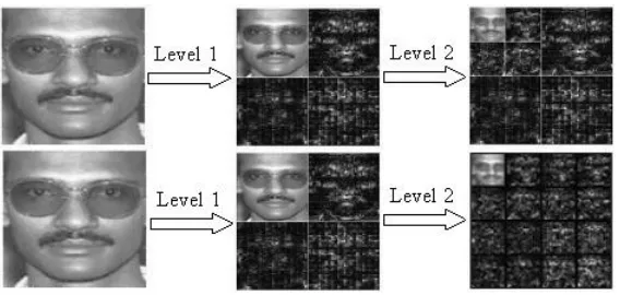
When dealing with images, the wavelet decomposition or the wavelet packet decomposition is first applied along the rows of the images, then their results are further decomposed along the columns. This results in four decomposed subimages L1, H1, V1 and D1. These subimages rep-resent different frequency localizations of the original image which refer to Low-Low, Low-High, High-Low and High-High respectively. Their frequency components comprise the original fre-quency components but now in distinct ranges. While the process being iterated, only L1is further decomposed in the wavelet decomposition, but all L1, H1, V1and D1are further decomposed in the wavelet packet decomposition. Figure 1 shows a two-dimensional examples of a facial image for the wavelet decomposition and the wavelet packet decomposition with depth 2.
2.2 The Local Discriminant Basis (LDB) Algorithm
The local discriminant bases algorithm (Coifman and Saito, 1994; Saito and Coifman, 1994, 1995) uses an adjustment of dictionary, or a wavelet packet decomposition tree which offers a library of orthonormal basis localized both in space and in frequency. Before proceeding further, let us set our notations. Let X={x1,x2,· · ·,xN}be an ensemble of training samples with K classes, X =
SK
y=1Xy,
and Xy ={xy1,x
y
2,· · ·x
y
Figure 1: (Top) The two-dimensional wavelet decomposition of facial image with depth 2. (Bottom) The two-dimensional wavelet packet decomposition of facial image with depth 2.
We use
D
to represent the space-frequency dictionary consisting of a collection of wavelet packet subbands {Bj}, j=1,· · ·,(4L+1−1)/3, where Bj ={bj1,bj2,· · ·,bjnj}, bji(i=1,2,· · ·,nj) arewavelet packet coefficients and njis the size of wavelet packet subband Bj,
L
is the decompositionlevel of wavelet packet.
The LDB algorithm first decomposes the training samples in the dictionary
D
, then sample energies at the basis coordinates are accumulated for each sample class separately to form a space-frequency energy distribution per class. Let Γ(y)(Bj) be a normalized energy of class y samplespresented on the subbands Bj:
Γ(y)
(Bj) = (Γ
(y)
(bj1),Γ
(y)
(bj2),· · ·,Γ
(y)
(bjnj)) ∀Bj⊂
D
, (1)Γ(y) (bjt)=∆
∑Ny
i=1
bjt·x
y
i
2
∑Ny
i=1kx
y
ik
2 (2)
where·denotes the standard inner product in the Euclidean space. The loss functionφ1is used to measure “distances” among K vectorsΓ(1)(Bj),Γ
(2)
(Bj),· · ·,Γ
(K) (Bj):
φ1(Bj) =φ1(Γ
(1) (Bj),Γ
(2)
(Bj),· · ·,Γ
(K)
(Bj))=∆
K
∑
m,n=1
m6=n
d∗(Γ(m)(Bj),Γ
(n)
(Bj)) (3)
where d∗(·,·) is a “distance” measure, it can be the l2 distance, the relative entropy, or the J-Divergence. Then φ1(Bj) will be a measure of efficacy of the subband Bj for classification, and
local discriminant basis are selected by the best-basis algorithm (Coifman and Wicherhauser, 1992) using the following criterion:
Ψ=arg max
B j∈Dφ1(Bj). (4)
2.3 The Modified LDB (MLDB) Algorithm
In Saito et al. (2002), a modified version of the LDB algorithm is introduced using the empirical probability distributions instead of the space-frequency energy distribution as their selection strategy to eliminate some less discriminant coordinates in each subband locally. Let
δjt=∆ φ2(Γ (1)
(bjt),Γ
(2)
(bjt),· · ·Γ
(K)
(bjt)) =
K
∑
m,n=1
m6=n
d∗(Γ(m)(bjt),Γ
(n)
(bjt)) (5)
that is, the discriminability of coordinate bjt (t=1,2,· · ·,nj). Then the measure of the
discrim-inability of Bj is obtained by summing only the n0(<nj)largest terms, that is,
φ2(Bj)=∆ n0
∑
t=1
δj(t) (6)
where{δj(t)}is the decreasing rearrangement of{δjt}, and local discriminant basis are selected by
the best-basis algorithm using the criterion (4) as LDB. The final step is the same as LDB.
Although the MLDB algorithm may overcome some limitations of LDB, the selection of coordi-nates is only limited to each subband so that coordicoordi-nates in different subbands are still incomparable.
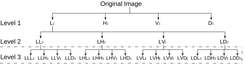
3. The General Framework of the LDC Algorithm
Our LDC algorithm uses a ternary architecture similar to LDB. We use the wavelet packet feature extraction at the first step. The main difference between LDB and our LDC algorithm is the nature of “distance” measure and feature selection strategy. We propose a new dilation invariant entropy to take the place of traditional traditional absolute “distance” measures. This ensures that the compar-ison of discriminability among all coordinates is independent of spatial frequency subbands. Thus, our selection can be based on all coordinates of the dictionary, but not the subbands themselves.
Moreover, LDB uses only the between-class difference, and ignores the within-class difference. This may lead to an unsatisfactory discriminability. The solution presented in this paper makes use of the maximum a posterior (MAP) logistic model. Its derived separability measure function will get a contrastive term to ensure not only the within-class difference is low, but also the between-class difference is large. Our LDC algorithm does not need the best-basis algorithm (Coifman and Wicherhauser, 1992) used in LDB, it ensures that we can select the most discriminant features with-out any impact of the best-basis algorithm. Subsequently, the LDC algorithm uses the complete linear discriminant analysis (CLDA) to solve the “small sample size” (SSS) problem, instead of the traditional LDA or CT in LDB. Finally, we modify the Euclidean distance and the cosine crite-rion in the nearest neighbor classifier, and replace them with the triangle square ratio critecrite-rion for classification.
3.1 The Wavelet Packet Decomposition in our LDC Algorithm
Original Image
L1 H1 V1 D1
Level 1
Level 2
Level 3
LL2 LH2 LV2 LD2
LLL3 LLH3 LLV3 LLD3 LHL3 LHH3LHV3 LHD3 LVL3 LVH3 LVV3 LVD3 LDL3 LDH3LDV3LDD3
Figure 2: The wavelet decomposition tree used in this study. The dashed part is the spatial-frequency dictionary
D
in the LDC algorithmSection 4, we will search for the most discriminant level by the best performance of its selected coordinates. Because it is more time-consuming when the decomposition level
L
is larger than 4,L
=4 will be used in the experiment. In the first level, four subband images—L1, H1, V1, D1—are obtained. However, the high frequency H1, V1, D1 are sensitive to noises in facial images, and Ekenel and Sanker (2005) claimed that they have low performance for classification. Moreover, the results in Table 4 show that our dilation invariant entropy used in the LDC algorithm may extract few high frequency components which may slightly affect the performance, also for the sake of computational efficiency, the H1, V1, D1components are not further decomposed. Our experimen-tal results show that Level 3 has better performance than Level 1, 2, 4, and the same results are also presented in Chien and Wu (2002). In fact, with the further wavelet packet decomposition, more fine scale information which may have good discriminant power is generated, however, the reso-lution of subband images becomes lower so that less information exists for the purpose of object localization (Grewe and Brooks, 1997). Neither little scale information nor little localization infor-mation can generate a judicious combination which has best discriminate power, so Level 3 which may give a suitable tradeoff between scale information and localization information is used in some studies (Chien and Wu, 2002; Feng et al., 2000). We also use Level 3 in the LDC algorithm, and our spatial-frequency dictionaryD
consists of 16 subbands in Level 3 (a subset of the dictionary in the LDB algorithm) (see Figure 2). The Daubechies db4 wavelet will be used for image decompo-sition (Daubechies, 1990), if the sizes of facial images are not the dyadic numbers, we will apply zero-padding extension to create the smallest dyadic images for the wavelet packet decomposition.3.2 The Dilation Invariant Entropy
In this subsection, we first point out the deficiency of absolute “distance” measures in wavelet-based methods, then introduce our dilation invariant entropy and its property.
3.2.1 DEFICIENCY OFABSOLUTE“DISTANCE” MEASURES IN WAVELET-BASEDMETHODS
-norm is defined by
ds`2(w,z)=∆ kw−zk22=
n
∑
i=1
(wi−zi)2. (7)
Suppose ∑ni=1wi =1,∑ni=1zi =1, then the Kullback-Leibler divergence (Kullback and Leibler,
1951), also known as relative entropy, is defined by
dKLD(w,z)=∆
n
∑
i=1 wilog
wi
zi
(8)
with the convention that log 0=−∞, logγ/0=∞forγ>0 and 0(±∞) =0. A symmetric version of dKLDis the J-Divergence (Kullback and Leibler, 1951) given by
dJDIV
(w,z)=∆ d
KLD(w,z) +dKLD(z,w)
2 . (9)
It is easy to show that measures in Equations (7)-(9) are additive discriminant measure, that is,
d∗(w,z) =
n
∑
i=1
d∗(wi,zi) (∗=s`2,KLD,JDIV). (10)
From Equations (3) and (10), we know that the discriminant measure of subband Bj in the LDB
algorithm can be written as
φ1(Bj) =
K
∑
m,n=1
m6=n
nj
∑
t=1
d∗(Γ(m)(bjt),Γ
(n)
(bjt)). (11)
Also from Equations (5) and (6), we know that the discriminant measure of subband Bj in the
MLDB algorithm can be written as
φ2(Bj) =
K
∑
m,n=1
m6=n
n0
∑
t=1
d∗(Γ(m)(bj(t)),Γ(n)(bj(t))),(n0<nj) (12)
where bj(t),(t=1,· · ·,n0)are the first n0coordinates with largest discriminability in subband Bj.
However, there are no normalized conditions imposed in each subband when the decomposition level
L
>0, because for each subband Bj(j>1)(B1is the original image)nj
∑
t=1
Γ(y) (bjt),
n0
∑
t=1
Γ(y)
(bj(t))<1 and
nj
∑
t=1
Γ(y)
(bjt)6≡C0, n0
∑
t=1
Γ(y)
(bj(t))6≡C1 ∀y
where C0,C1are constants independent of y and Bj. Without the normalized conditions, the absolute
“distance” measures (7)-(9) will lead to a jeopardy thatφ1(Bj)andφ2(Bj)depend absolutely on the
order of magnitude (OM) ofΓ(m)(bjt),Γ
(n)
(bjt)andΓ
(m)
(bj(t)),Γ
(n)
(bj(t))respectively.
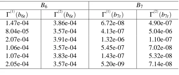
B6 B7
Γ(1)
(b6t) Γ(2)(b6t) Γ
(1)
(b7t) Γ
(2) (b7t) 1.47e-04 3.86e-04 6.72e-08 4.90e-07 8.04e-05 3.57e-04 4.13e-07 5.04e-06 2.07e-04 3.91e-04 1.32e-06 1.10e-07 1.06e-04 3.57e-04 5.45e-07 7.02e-08 1.07e-04 3.83e-04 1.43e-07 5.32e-08 2.05e-04 3.57e-04 5.20e-09 7.14e-08
Table 1: Values ofΓ(y)(b6t),Γ (y)
(b7t) (y=1,2; t=1,· · ·,6)
Figure 2) of the second level may vary from 0.001 to 0.01. Table 1 lists an example of some values ofΓ(y)(b6t),Γ(y)(b7t)computed by Equation (2) in latter experiment.
From Equations (11),(12) and (2), we can deduce a bad result that the coordinates in lower spatial frequency subbands have more discriminability because of the larger OM of theirs loadings, and the coordinates in higher spatial frequency subbands have less discriminability because of the smaller OM of theirs loadings. So the low spatial frequency subbands are dominant in the LDB and MLDB algorithm. However, it is unreasonable to neglect the middle and high spatial frequency components merely for small OM of their loadings. Our experimental results also show that not only low spatial frequency components, but also middle spatial frequency components are useful for face recognition.
3.2.2 THEDILATIONINVARIANT ENTROPY ANDITSPROPERTY
First, we define that the separability of sample ensemble X is the probability of classifying all sam-ples into their genuine classes by certain discriminant functions. It is well-known that the separabil-ity of X does not depend on the absolute distances based on the OM of sample values, but depends on the relative distances among all the samples in X . For each coordinate c, the coordinate loadings from all the training samples can induce a sample ensemble Xc inR1, and the discriminability of c is equivalent to the separability of Xc, so it is independent of the OM of coordinate loadings, and only depends on the relative distances among the coordinate loadings from all the training samples. Obviously, the “distance” measures used in LDB do not take this fact into account. So we propose a new “distance” measure derived from the J-Divergence. We call it the dilation invariant entropy :
dDIE
(w,z)=∆
n
∑
i=1 1 2(wi+zi)
(wi zi
log wi+
zi
wi
log zi) = n
∑
i=1
(wi−zi)(log wi−log zi)
2(wi+zi)
(13)
where w= (w1,w2,· · ·,wn), z= (z1,z2,· · ·,zn)are two nonnegative sequences, with the convention
that log 0=−∞, logγ/0=∞forγ>0 and 0(±∞) =0.
Proposition 1 The new relative entropy defined by Equation (13) is dilation invariant.
dDIE
(f(w),f(z)) =dDIE
(aw,az) =
n
∑
i=1
(awi−azi)(log awi−log azi)
2(awi+azi)
=
n
∑
i=1
a(wi−zi)(log wi+log a−log zi−log a)
2a(wi+zi)
=
n
∑
i=1
(wi−zi)(log wi−log zi)
2(wi+zi)
=dDIE
(w,z).
In fact, the new dilation invariant entropy is the generalization of the J-Divergence (when the J-Divergence satisfies the constraint: w+z=1)because
dDIE
(w,z) =
n
∑
i=1
(wi−zi)(log wi−log zi)
2(wi+zi)
=
n
∑
i=1 1 2(
wi
wi+zi
− zi
wi+zi
)(log wi
wi+zi
−log zi wi+zi
)
=1
2(
n
∑
i=1
w0ilogw
0
i
z0i +
n
∑
i=1 z0ilog z
0
i
w0i)
=dJDIV(w0,z0)
(14)
where w0i= wi
wi+zi,z 0
i=wiz+izi, w 0
i+z0i=1 and w0= (w01,· · ·,w0n),z0= (z01,· · ·,z0n). Equation (14) shows
that the dilation invariant entropy normalizes the sample ensembles into unit sample ensembles with the sum formalism, so different sample ensembles are comparable for their separability. Similarly, we can define the dilation invariant`2norm as
dDI`2
(w,z) =
n
∑
i=1 ( wi
wi+zi
− zi
wi+zi
)2
!12
=
n
∑
i=1
(w0i−z0i)2
!12
=d`2(w0,z0). (15)
In Section 4, we will conduct an experiment to test the performance of the LDC algorithm using both dilation invariant entropy and dilation invariant`2norm.
The dilation-invariance of the new relative entropy ensures that the separability of each coordinate-loadings ensemble Xcis independent of its OM. Accordingly, the discriminability of each coordinate c can be independent of its corresponding subband. It offers a benefit that any two coordinates in the dictionary
D
are comparable for their discriminability. So all the coordinates in the dictionary can be uniformly selected by a criterion.3.3 Feature Selection Criterion
3.3.1 THEMAXIMUMa posteriori (MAP) LOGISTICMODEL
To select the most discriminant coordinates, we make use of the Bayesian algorithm based on min-imizing the error on the training set. The Bayesian algorithm adopts a probabilistic measure of similarity based on a Bayesian MAP analysis of face differences. In the traditional methods (Wang et al., 2006; Chou, 2000), the similarity measure is used to characterize what kind of image variation is typical for the same person and what is for different persons. In this paper, the MAP similarity measure is used to choose the coordinates that make the training data set with known class labels having the minimum error. In this way the selected coordinates can make the known classification of training data set the most probable:
ˆ
c=arg max
c K
∑
y=1 1 #(Xy)
Z
X
Pc(Xy|x)1(x∈Xy)dP(x)
where #(·) is the cardinal number, and 1(·) is the indicator function. The posterior probability Pc(Xy|x)can be rewritten as
Pc(Xy|x) =Pc(x|Xy)Pc(Xy)/Pc(x) =Pc(x|Xy)Pc(Xy)/P(x).
Since P(x)is not a function of the class index and thus has no effect in the MAP decision, the needed probabilistic knowledge can be represented by the class prior distribution Pc(Xy)and the conditional
probability Pc(x|Xy)which will be modeled by logistic functions.
Definition 1 The prior distribution Pc(Xy)is defined as
Pc(Xy) =
1 T
1 1+exp(−dDIE(Γ(y)
(c),Γ(0) (c))),
T=
K
∑
y=1
1 1+exp(−dDIE(Γ(y)
(c),Γ(0) (c))).
(16)
Definition 2 The conditional probability Pc(xyi|Xy)(x=xyi)is defined as
Pc(xyi|Xy) =
1
1+exp(dDIE(Γi(y)(c),Γ(y)
(c)) (17)
whereΓ(y)(c)is defined by Equation (2), representing the normalized spatial-frequency energy map of class y on coordinate c, and can be thought of as the center of class y. Similar to that of LDB, we set
Γ(y)
i (c)
∆
=|c·x
y
i|
2
kxyik2 , Γ
(0)
(c)=∆ ∑
K
y=1∑
Ny
i=1|c·x
y
i|
2
∑K
y=1∑
Ny
i=1kx
y
ik
2 . (18)
Γ(y)
i (c) represents the normalized spatial-frequency energy map of sample x
y
i on coordinate c, and
Γ(0)(c)represents the normalized spatial-frequency energy map of all the training samples on coor-dinate c, which can be considered as the center of all samples.
The properties of the probability functions Pc(Xy)and Pc(xyi|Xy)can be made clear by
consider-ing the sigmoid function:
f(d) = 1
with θnormally set to zero and γset to 1 for Pc(Xy) and -1 for Pc(xyi|Xy). Whenγ=1, f(d) is
a monotonically increasing function, a larger dDIE(Γ(y)(c),Γ(0)(c)))means that it is more probable to separate class set Xy. Contrarily, whenγ=−1, f(d) is a monotonically decreasing function, a
smaller dDIE(Γ(iy)(c),Γ(y)(c))means that sample xyi is more likely to belong to class set Xy. In fact,
the idea of MAP logistic model is derived from the Fisher criterion. Moreover, the sigmoid function can effectively allay the effect of outliers which have great effect on the Fisher criterion.
3.3.2 SEPARABILITYMEASURE ANDFEATURESELECTIONCRITERION
For the given training data set, the empirical probability measure P(x)defined on the training data set is a discrete probability measure that assigns equal mass at each sample. We define the separability measure as
SM(c) =
K
∑
y=1 1 #(Xy)
Z
X
Pc(Xy|x)1(x∈Xy)dP(x)
≈ K
∑
y=1 1 Ny
Ny
∑
i=1
Pc(xyi|Xy)Pc(Xy)
=
K
∑
y=1 Pc(Xy)
1 Ny
Ny
∑
i=1
Pc(xyi|Xy)
!
.
(19)
In fact, the separability measure defined by Equation (19) is an empirical measure. If the training samples are obtained by an independent sampling from a space with a fixed probability distribution P0(x), the empirical probability distribution P(x)will converge to P0(x)in distribution as N →∞. Then the empirical measure defined on the N independent training samples will converge to the expected measure as the sample size N increases. With sufficient training samples, the empirical measure is an estimate of the expected measure. The goodness of this estimate is determined by the training sample size N and the convergence rate of the empirical probability measure P(x)to the limit distribution P0(x).
Furthermore, we use the following criterion for feature selection:
Criterion: Select uniformly the first N0coordinates from the dictionary
D
with largest separability measure defined by Equation (19).3.4 Discriminant Analysis
LDA (Fukunaga, 1990) is a linear statistic classification method, which tries to find a linear trans-form so that after its application the scatter of sample vectors is minimized within each class and the scatter of mean vectors around the total mean vector is maximized simultaneously.
Let the between-class scatter operator Sband the within-class scatter operator Swbe:
Sb=
1 N
K
∑
y=1
Ny(my−m0)(my−m0)T, Sw=
1 N
K
∑
y=1
Ny
∑
i=1
(xyi−my)(xyi−my)T
where my is the mean of the mapped training sample of class y, and m0 is the mean across all the
J1(ϕ1) =
ϕT
1Sbϕ1
ϕT
1Swϕ1
, (ϕ16=0,kϕ1k=1). (20) The solution to maximizing J1(ϕ1)can be found by searching for a direction which maximizes the projected class means (the numerator) while minimizing the class variances in this direction (the denominator).
However, the LDA algorithm often suffers from the “small sample size” (SSS) problem which exists in high-dimensional pattern recognition tasks, where the number of available samples is smaller than the dimensionality of the samples. Many methods (Mika et al., 1999; Baudat and Anouar, 2000; S. Mika and M ¨uller, 2003; Yang, 2002) discard the discriminant information con-tained in the null space of Sw. But a significant result is a finding that there exists crucial
discrim-inative information in the null space of Sw (Chen et al., 2000; Zhuang and Dai, 2007; Yang and
Yang, 2003; Yu and Yang, 2001). We proposed the use of regularization (Dai and Yuen, 2003), but it involves a determination of parameters. Yang et al. (2005) proposed a complete kernel Fisher discriminant analysis algorithm which makes full use of two kinds of discriminant information, reg-ular and irregreg-ular in kernel feature space. Its advantage is that no estimation of parameter is needed. Based on their idea, we use complete linear discriminant analysis (CLDA) in the LDC algorithm to solve the SSS problem.
In Equation (20), if the within-class scatter operator Swis invertible,ϕT1Swϕ1>0 always holds for every nonzero vectorϕ1, and the Fisher criterion can be directly employed to extract a set of optimal discriminant vectors. If Sw is singular, there always exist vectors satisfying ˜ϕTSwϕ˜ =0.
These vectors are from the null space of Sw (null(Sw)) and can be very effective if they satisfy
˜
ϕTS
bϕ˜ >0 at the same time (Chen et al., 2000; Zhuang and Dai, 2007; Yang and Yang, 2003; Yu
and Yang, 2001). In this case, the Fisher criterion degenerates into the following between-class scatter criterion:
J2(ϕ2) =ϕT2Sbϕ2, (kϕ2k=1). (21) CLDA uses the between-class scatter criterion defined in Equation (21) to derive the irregular dis-criminant vectors from null(Sw), while using the standard Fisher criterion defined in Equation (20)
to derive the regular discriminant vectors from range(Sw).
In our experiments, we capture all the regular discriminant vectors which satisfy J1(ϕ1)>0 from the range space of Sw, simultaneously, we capture all the irregular discriminant vectors which
satisfy J2(ϕ2)>0 from the null space of Sw.
3.5 A New Criterion for the Nearest Neighbor (NN) Classifier
ratio which takes into account of both distance and correlation between two vectors. Supposeυ1,
υ2are two vectors, the triangle square ratio is defined as
T SR(υ1,υ2) = kυ1−υ2k 2 2
kυ1k22+kυ2k22 .
The triangle square ratio is a similarity measure based on the argument and modulus of each vector, as shown in proposition 2.
Proposition 2 Suppose θis the include angle ofυ1 and υ2, then T SR(υ1,υ2)→0 if and only if
kυ1k2→ kυ2k2andθ→0, which implies the correlation betweenυ1andυ2should approach 1. Proof
T SR(υ1,υ2) =1−2kυ1k2· kυ2k2 kυ1k22+kυ2k22
cosθ (by the cosine law)
≥1−cosθ (“=” holds if and only if kυ1k2=kυ2k2)
≥0 (“=” holds if and only if θ=0).
(22)
In fact, ifυ1 andυ2 are unit vectors, the triangle square ratio is equivalent to Euclidean distance. Also, Equation (22) shows that triangle square ratio is a modification of cosine criterion by the term 2kυ1k2·kυ2k2
kυ1k22+kυ2k22
. Ifkυ1k2=kυ2k2, it is equivalent to cosine criterion. Moreover, we have done large numbers of numerical experiments which exclusively show that pT SR(υ1,υ2) satisfies the triangle inequality, and the symmetric and positive definitive properties are obvious. So we guess
p
T SR(υ1,υ2)is a distance measure, its proof in theory is an open problem.
Experimental results in Section 4 show that the triangular square ratio is more robust against illumination variations than the Euclidean distance, whilst retaining the robustness against pose and expression changes as the Euclidean distance. On the other hand, although the triangular square ratio marginally underperforms the cosine criterion when there are variations of illumination, it can obviously outperform the cosine criterion when there are changes of pose and expression.
3.6 The Procedure of Proposed LDC Algorithm
We summarize our local discriminant wavelet packet coordinates algorithm as follows: Step 1: The wavelet packet transform
Expand each training sample xy
i into the spatial-frequency dictionary
D
(see Figure 2) bythe wavelet packet decomposition, then xyi will be represented by the loadings of coordinates in
D
. Step 2: The LDC selection transform(2.a) For each coordinate c in the dictionary
D
, use the Equations (2), (18), (16), and (17) to compute its prior distribution Pc(Xy)and conditional probability Pc(xyi|Xy), whereafter, compute itsseparability measure defined by Equation (19), that is, its discriminability.
(2.b) Select the first N0coordinates from
D
with the largest discriminability. Whereupon, each training sample xyi can be represented by a feature vector v
y
i which is formed by the loadings of the
Use the Equations (20) and (21) to construct the subspace template by the complete linear dis-criminant analysis (CLDA) in
F
.Step 4: Testing a new probe sample
For a new probe sample, it will be expanded into the spatial-frequency dictionary
D
by the wavelet packet decomposition, and be extracted the loadings of the corresponding coordinates se-lected in Step 2 to form a new feature vector vnew. Then vnew will be projected to the subspaceconstructed in Step 3 and classified by the nearest neighbor classifier. Simply, the LDC algorithm can be represented as:
Out put=T3·T2·T1·Input
where T1is the wavelet packet transform, T2is the LDC selection transform. and T3 is the CLDA transform.
3.7 Computational Complexity Comparison of the LDC and LDB Algorithm
The framework of the LDC algorithm is similar to LDB. We compare their computational complex-ity step by step:
Step 1: The wavelet packet transform
The same procedure of the LDC and LDB algorithms cost O(N·nrnc·
L
), where nr×nc is thesize of facial images,
L
is the level of the wavelet packet decomposition. Step 2: The LDC/LDB selection transform(2.a) For each coordinate in
D
LDC, the LDC algorithm needs to compute the prior distribution(16), the conditional probability (17) and its discriminability (19), so the costs of all the coordinates in
D
LDC are O(N·nrnc) +O(K·nrnc) +O(N·nrnc). For each subband inD
LDB, the LDB algorithmneeds to compute the space-frequency energy distribution (2), (1) and its measure of efficacy (3). So the costs of all the subbands in
D
LDBare O(N·nrnc·L
) +O(K2·nrnc·L
).(2.b) The LDC algorithm needs to sort all the coordinates in
D
LDC by their discriminability,which costs O(nrnc·log2(nrnc)). The LDB algorithm needs to select the local discriminant basis
from
D
LDB using the best-basis algorithm, which costs O(L
·4L). Then both algorithms need torepresent all the training samples by new feature vectors, which cost O(N·N0). Step 3: The CLDA/LDA transform
CLDA in the LDC algorithm has the same computational complexity O((N0)3)as LDA in the LDB algorithm in the new feature space
F
.Step 4: Testing a new probe sample
A new probe sample should be transformed by T1, T2, T3with complexity O(nrnc·
L
) +O(N0) + O(N0·Nev)and classified by the NN classifier with complexity O(N·Nev), where Nevis the numberof eigenvectors extracted by CLDA or LDA.
The computational complexity of Step 2 shows that the LDC algorithm is more efficient than LDB in many real applications when K is large. Table 11 also validates the fact.
4. Experiment Results
of the LDC based feature extraction, the complete linear discriminant analysis (CLDA) and the nearest neighbor (NN) classifier with the triangle square ratio (T SR) criterion. In the second and third parts, we evaluate the efficacy of the LDC feature extraction and the new classifying criterion respectively. The fourth part gives the performance of the whole LDC algorithm. Some further researches of the LDC algorithm are shown in the final part.
4.1 Database
1) FERET Database: The FERET database, distributed by the National Institute of Standards and Technology, consists of 14051 eight-bit grayscale images of human heads with different expres-sions, poses, occlusion and illuminations (Phillips et al., 2000). Two data sets of the database are used in our experiments, one is a small data set, which contains 432 images of 72 people and each individual has six images, the other is a large data set with 255 individuals, and each person has four frontal images, the datas are extracted from four different sets, namely, Fa, Fb, Fc, and duplicate (Phillips et al., 2000). There are 1020 images in this data set. All the images are aligned by the centers of eyes and mouth, and then normalized with the resolution 92×112. Some images from both data sets of the FERET database are shown in Figure 3.
2) ORL Database: The Olivetti-Oracle Research Lab (ORL) database has 40 subjects and each subject has 10 different facial views representing various expressions, small occlusion (by glasses), different scales and orientations. So there are totally 400 facial images in the database. Each image has 92×112 pixels in gray scale. Some samples are shown in Figure 4.
3) Hybrid Database: As aforementioned, the variations of the ORL database and the FERET database are very different, which lead to unequal covariance distribution. So we blend the small FERET data set and the ORL database together, in order to test the performance of the LDC algo-rithm when facial images have larger illumination variations and pose, expression changes (Loog and Duin, 2004). The hybrid database has 832 images of 112 persons.
4) CMU PIE Database: The CMU Pose, Illumination, and Expression (PIE) (Sim et al., 2003) database consists of 41368 images of 68 people. Each person has images captured under 13 different poses and 43 different illumination conditions and with four different expressions. In this paper, we use a subset that focuses on illumination variations with pose and expression variations in frontal
Figure 4: Segmental facial images of one person. (Top) From the ORL database. (Bottom) From the CMU PIE database.
Total number Number of images Number of Database
of images per person classes
ORL 400 10 40
SmallFERET 432 6 72
LargeFERET 1020 4 255
Hybrid 832 6 or 10 112
CMU-lights 2924 43 68
Table 2: Statistics for face images
view. There are 68 persons with each 43 images yielding a total of 2924 images. Each image has 92×112 pixels in gray scale. Some samples are shown in Figure 4.
The statistics of each data set is listed in Table 2.
4.2 Parameter Setting
In order to show more comparability with the PCA+CLDA, WaveletFace, LDB and MLDB algo-rithms and present the performance of our LDC algorithm more accurately, CLDA is used to capture the complete discriminant features in the five algorithms. The number of discriminant vectors is ob-tained in the same way as the LDC algorithm (see Subsection 3.4).
The FisherFace technique uses the classical PCA+LDA. The Ntrain−K−λ(λis the critical value
which ensures Swis non-singular) eigenvectors with largest eigenvalues are preserved on ‘PCA step’
(Belhumeur et al., 1997). For the PCA+CLDA algorithm, we select the first min(N0,M0)(M0is the number of non-zero eigenvalues) eigenvectors with largest eigenvalues on ‘PCA step’. For direct LDA (DLDA), we use all the eigenvectors in their Step 2 (Yu and Yang, 2001).
The third-level lowest frequency subband LLL3with a matrix of(nr/8)×(nc/8)(where nr×nc
Parameters Methods
number of features for discriminant analysis classifier (criterion) FisherFace Ntrain−K−λ NN(l2)
PCA+CLDA min(N0,M0) NN(l2)
DLDA all eigenvectors NN(l2)
WaveletFace subband LLL3in
D
NN(l2)LDB four subbands NN(l2)
MLDB 5×260 NN(l2)
LDC N0 NN(T SR)
Table 3: Parameters of aforementioned methods
In the ‘Decision Step’, we use the nearest neighbor classifier with the Euclidean distance for the aforementioned methods as their original forms. For our LDC algorithm, we use the new triangle square ratio criterion, the Euclidean distance and the cosine criterion are used for comparison. Most parameters are listed in Table 3.
The recognition rate is calculated as the ratio of the number of successful recognition and the total number of test samples. All the experiments are repeated 30 times, and the final recognition rate is the average value of the thirty results. Suppose M is the number of facial images for each person. On each database, we randomly select i0(<M)images from each person for training, while the rest M−i0 images of each individual are selected for testing. i0 is a small integer, in order to show the performance of the LDC algorithm when there are small-size-training samples.
4.3 Construction of the Dictionary
D
and Choice of N0In this subsection, we conduct two experiments to construct the dictionary
D
and select a suitable N0for the LDC algorithm.4.3.1 CONSTRUCTION OF THEDICTIONARY
D
In the first experiment, to construct our dictionary
D
, we search for the most discriminant level by the best performance of its selected coordinates. Because it is more time-consuming when the decomposition levelL
is larger than 4,L
=4 is used in the experiment. In order to test the effect of high frequency components and show the tolerance of the dilation invariant entropy in LDC to noise, we design two schemes: Scheme 1 uses all the subbands in the wavelet decomposition tree, Scheme 2 only uses the left subtree whose root node is L1, that is the H1, V1, D1components are not further decomposed. For each level, we select the first 1000 coordinates by the criterion in Subsection 3.3 for both schemes. Their performances on the small FERET data set and the ORL database are shown in Table 4.Training Level Database
samples (i0)
Schemes
1 2 3 4
1 82.43±2.40 91.38±2.57 92.99±1.60 90.43±2.38 3
2 82.35±2.54 92.19±2.32 93.30±1.85 92.34±1.78 1 85.54±2.76 94.00±1.56 94.47±1.68 91.79±2.08
ORL 4
2 85.56±2.87 94.43±1.62 95.26±1.46 94.18±1.35 1 87.70±2.03 95.32±1.45 95.42±1.71 92.57±1.62 5
2 87.82±2.12 96.03±1.49 96.23±1.55 94.12±1.59 1 92.42±1.93 91.88±1.69 92.33±2.51 92.41±2.42 3
2 92.42±1.93 91.88±1.77 92.30±2.43 92.53±2.39 FERET 1 94.93±1.40 94.79±2.25 95.23±2.40 94.31±2.58 (small) 4 2 94.93±1.40 94.72±2.04 95.60±2.20 95.30±2.94 1 95.93±1.41 96.30±1.76 97.04±1.92 96.39±2.95 5
2 95.93±1.41 96.07±1.90 96.90±2.33 97.13±2.13 (∗)±(∗∗): (∗) represents the recognition rate (%), (∗∗) represents standard deviation (%).
Table 4: Effect of high frequency components and performances of level 1,2,3,4
scale information and localization information. So Level 3 is used in the LDC algorithm, and our spatial-frequency dictionary
D
consists of the first 16 subbands in the third level (see Figure 2).4.3.2 CHOICE OFN0
Because all of the top N0 coordinates are used for the classification, a natural way to determine the best N0 is to select the top N0 coordinates and compute the average recognition rates for various different N0. Based on the idea, we use a global to local search strategy (M ¨uller et al., 2001) on both data sets of the FERET database. Because the computational complexity of CLDA is O((N0)3), for the sake of computational efficiency, we set the range [100,2500] as the original wide range of N0. In the “global” stage, we compare the performances of the LDC algorithm using the top N0coordinates when N0increases from 100 to 2500 with interval 100 on the small data set, as shown in Figure 5 (Left). It shows that the LDC algorithm has a good and stable performance after N0=700 because more good discriminant features are used. After N0=1700, the performance slightly decreases due to the more redundant information included. So we ascertain a more precise subrange [700, 1700] where the optimal N0might exist.
In the “local” stage, we compare the performances of different N0between 700 and 1700 with interval 100 on the large data set, as shown in Figure 5 (Right). From the overall comparison of two stages, we find that when N0increases from 1300 to 1700 with interval 100, their performances are very close, and the performance of N0=1300 is marginally better than others. Also for the sake of computational efficiency, we select the first N0=1300 best discriminant coordinates in our following experiments.
1 3 5 7 9 11 13 15 17 19 21 23 25 0.82
0.84 0.86 0.88 0.9 0.92 0.94 0.96 0.98 1
N
0=700 N0=1700
N 0/100
Recognition rate
3 training samples 4 training samples 5 training samples
7 8 9 10 11 12 13 14 15 16 17 0.84
0.86 0.88 0.9 0.92 0.94 0.96 0.98
N0=1300
N 0/100
Recognition rate
2 training samples 3 training samples
Figure 5: (Left) The performances of the LDC algorithm using different N0between 100 and 2500 with interval 100 on the small FERET data set. (Right) The performances of the LDC algorithm using different N0between 700 and 1700 with interval 100 on the large FERET data set.
13 14 15 16 17
0.92 0.94 0.96 0.98 1
N 0/100
Recognition rate
3 training samples 4 training samples 5 training samples
13 14 15 16 17
0.9 0.92 0.94 0.96 0.98 1
N 0/100
Recognition rate
3 training samples 6 training samples 9 training samples
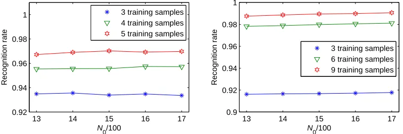
Figure 6: The performances of the LDC algorithm using different N0between 1300 and 1700 with interval 100. (Left) The ORL database. (Right) The CMU-lights database.
4.3.3 RECONFIRMATION OF THEDICTIONARY
D
USINGN0=1300Moreover, we return to the anterior experiment (the construction of the dictionary
D
) with the top N0(=1300)coordinates. The results prove that the third level has the best performance once again, as shown in Figure 7.4.4 Efficacy of the LDC Based Feature Extraction
3 4 5 0.82
0.85 0.88 0.91 0.94 0.97
Training Samples
Recognition rate
Level 1 Level 2 Level 3 Level 4
3 4 5
0.92 0.93 0.94 0.95 0.96 0.97 0.98
Training Samples
Recognition rate
Level 1 Level 2 Level 3 Level 4
Figure 7: Performances of the LDC algorithm with N0(=1300) coordinates in four levels. (Left) The ORL database. (Right) The small FERET data set.
Training Methods with the l2criterion
Database samples (i0) LDC LDB MLDB WaveletFace
3 93.43±1.95 93.30±2.22 92.49±1.91 92.92±1.60 ORL 4 95.81±1.59 95.60±1.53 95.18±1.39 94.56±1.77 5 96.95±1.59 96.65±1.20 96.43±1.29 94.20±1.82 3 89.63±3.01 87.56±3.29 84.23±3.26 88.80±3.47 FERET
4 92.92±4.57 91.90±4.48 88.80±4.11 85.74±4.85 (small)
5 96.11±3.39 95.69±3.29 93.01±3.80 87.50±3.28 FERET 2 79.53±3.23 76.05±2.90 67.16±3.36 73.18±4.77 (large) 3 89.32±1.82 87.45±1.94 79.69±1.99 72.59±4.14 3 79.46±10.95 79.92±10.91 81.30±9.87 78.44±10.92
CMU-6 93.48±7.63 93.69±7.52 94.16±6.89 85.08±7.79 lights
9 96.83±4.29 96.54±4.50 96.76±4.56 54.80±17.52
Table 5: Comparison with wavelet-based methods
extraction in LDC with other wavelet-based methods, such as LDB, MLDB and WaveletFace on the ORL database, both data sets of the FERET database and the CMU-lights database. The setting of the feature extractions can be seen in Subsection 4.2. In order to show more comparability, all the methods use CLDA and the NN classifier with the Euclidean distance.
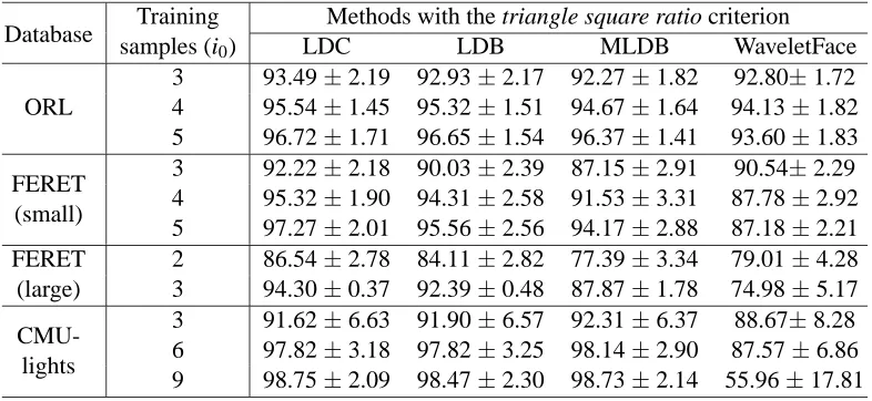
Training Methods with the triangle square ratio criterion Database samples (i
0) LDC LDB MLDB WaveletFace 3 93.49±2.19 92.93±2.17 92.27±1.82 92.80±1.72 ORL 4 95.54±1.45 95.32±1.51 94.67±1.64 94.13±1.82 5 96.72±1.71 96.65±1.54 96.37±1.41 93.60±1.83 3 92.22±2.18 90.03±2.39 87.15±2.91 90.54±2.29 FERET
4 95.32±1.90 94.31±2.58 91.53±3.31 87.78±2.92 (small)
5 97.27±2.01 95.56±2.56 94.17±2.88 87.18±2.21 FERET 2 86.54±2.78 84.11±2.82 77.39±3.34 79.01±4.28 (large) 3 94.30±0.37 92.39±0.48 87.87±1.78 74.98±5.17 3 91.62±6.63 91.90±6.57 92.31±6.37 88.67±8.28
CMU-6 97.82±3.18 97.82±3.25 98.14±2.90 87.57±6.86 lights
9 98.75±2.09 98.47±2.30 98.73±2.14 55.96±17.81
Table 6: Efficacy of the triangle square ratio criterion
4.5 Efficacy of the Triangle Square Ratio Criterion
Classifier and its classifying criterion are also important elements for face recognition. Generally, distance-based criterion is more robust than correlation-based criterion with respect to pose and expression changes while the contrary result is shown with respect to illumination variations. To extend the capacity covering variations of pose, expression and illumination, we have proposed the new triangle square ratio criterion in Subsection 3.5. In this experiment, we use the same four feature extractions and CLDA as in Subsection 4.4, but the Euclidean distance is replaced by the triangle square ratio criterion for the NN classifer. The results on the ORL database, both data sets of the FERET database and the CMU-lights database are shown in Table 6.
Comparing the results on Table 6 with Table 5 which uses the Euclidean distance, it shows that the triangle square ratio criterion performs better than the Euclidean distance considerably on both data sets of the FERET database and the CMU-lights database, while its efficacy is very close to the Euclidean distance on the ORL database. In fact, the FERET database, the CMU-lights database concern about illumination variations (light intensity and direction respectively), and the ORL database concerns about expression and pose changes. Comparison results show that the trian-gle square ratio criterion is more robust against illumination variations than the Euclidean distance, whilst retaining the robustness against pose and expression changes as the Euclidean distance.
Furthermore, we replace the triangle square ratio criterion with the cosine criterion, whilst keeping the other setting, on the ORL database and the small FERET data set. The performance of the cosine criterion is showed in Table 7. The comparison between Table 6 and Table 7 shows that the triangle square ratio criterion performs better than the cosine criterion considerably on the ORL database, although it marginally underperforms the cosine criterion on the small FERET data set.
4.6 Performance of the LDC Algorithm
Training Methods with the cosine criterion Database samples (i
0) LDC LDB MLDB WaveletFace 3 92.54±1.93 91.56±2.12 90.99±2.03 91.88±1.73 ORL 4 94.78±1.42 94.25±1.50 93.71±1.71 93.46±1.89 5 96.22±1.60 96.00±1.49 95.53±1.58 93.73±1.76 3 92.41±1.97 90.15±2.56 86.99±3.00 90.82±2.58 FERET
4 95.67±1.96 94.86±2.31 91.85±3.29 87.94±3.51 (small)
5 97.27±2.01 95.56±2.43 94.49±2.62 87.55±2.59
Table 7: Performance of the cosine criterion
Since our motivation is to compensate for illumination, pose and expression variation, from the properties of various databases, the ORL database is used to test moderate variations in pose and expression, the CMU-lights database to test illumination variations, the FERET database for more generic situation, and the hybrid database to test heteroscedastic class covariance distribution tolerance.
4.6.1 COMPARISON ON THEINDIVIDUALDATABASES
The comparison of results are depicted in Table 8. Although some algorithms occasionally have better performance, LDC shows stable performance for every number of training samples per class on all databases. Especially on the large FERET data set, it outperforms FisherFace, PCA+CLDA, DLDA, WaveletFace, LDB, MLDB by 30.94%, 10.49%, 31.85%, 13.36%, 10.49%, 19.38% respec-tively when two samples per class are used for training, and by 21.75%, 5.95%, 31.75%, 21.71%, 6.85%, 14.61% respectively when three samples per class are used for training. In particular, LDC significantly outperforms FisherFace, DLDA, WaveletFace. From the standard derivation, we can see that LDC has better stability than other algorithms.
4.6.2 COMPARISON ON THEHYBRIDDATABASE
On the hybrid database, we randomly select i0(i0=2 to 4) images from each person for training, the rest (6−i0) images of each individual in the small FERET data set are tested while the rest (10−i0) images of each individual in the ORL database are used for testing. The comparison results are recorded in Table 9.
It shows that when the number of training sample per class increases from 2 to 4, the average recognition rates of LDC are from 82.20% to 90.28%. The performance is better than Fisher-Face, PCA+CLDA, DLDA, WaveletFisher-Face, LDB and MLDB which increase from 60.38%, 79.06%, 66.86%, 77.43%, 77.99%, 76.00%, to 75.63%, 90.64%, 80.85%, 66.09%, 88.11%, 86.09% respec-tively on the hybrid database.
Training samples (i0)
Database Methods 3 4 5
FisherFace 87.20±1.96 90.53±1.87 92.07±1.97 PCA+CLDA 91.89±1.97 94.81±1.68 96.48±1.58 DLDA 84.17±2.23 87.31±1.92 90.17±1.55 ORL WaveletFace 92.92±1.60 94.56±1.77 94.20±1.82 LDB 93.30±2.22 95.60±1.53 96.65±1.20 MLDB 92.49±1.91 95.18±1.39 96.43±1.29 LDC(T SR) 93.49±2.19 95.54±1.45 96.72±1.71 FisherFace 84.85±3.64 88.01±4.91 91.94±4.23 PCA+CLDA 89.07±2.88 92.85±4.06 95.60±3.95 DLDA 80.45±4.81 86.34±5.28 88.61±6.41 FERET
WaveletFace 88.80±3.47 85.74±4.85 87.50±3.28 (small)
LDB 87.56±3.29 91.90±4.48 95.69±3.29 MLDB 84.23±3.26 88.80±4.11 93.01±3.80 LDC(T SR) 92.22±2.18 95.32±1.90 97.27±2.01
Training samples (i0)
2 3
FisherFace 55.60±5.10 72.55±2.57 PCA+CLDA 76.05±3.36 88.35±1.74 DLDA 54.69±4.86 62.55±2.30 FERET
WaveletFace 73.18±4.77 72.59±4.14 (large)
LDB 76.05±2.90 87.45±1.94 MLDB 67.16±3.36 79.69±1.99 LDC(T SR) 86.54±2.78 94.30±0.37
Training samples (i0)
3 6 9
FisherFace 80.57±8.96 94.46±6.44 97.36±4.08 PCA+CLDA 78.48±10.89 93.91±7.72 97.45±3.70 DLDA 76.92±7.48 87.49±6.60 92.65±4.60
CMU-WaveletFace 78.44±10.92 85.08±7.79 54.80±17.52 lights
LDB 79.92±10.91 93.69±7.52 96.54±4.50 MLDB 81.30±9.87 94.16±6.89 96.76±4.56 LDC(T SR) 91.62±6.63 97.82±3.18 98.75±2.09
Table 8: Comparison on the individual databases
4.7 Some Further Researches of the LDC Algorithm
Training samples (i0) Methods
2 3 4
FisherFace 60.38±3.24 72.58±2.51 75.63±2.87 PCA+CLDA 79.06±2.22 86.99±1.34 90.64±1.77 DLDA 66.86±2.57 74.55±2.61 80.85±1.89 WaveletFace 77.43±2.28 76.21±1.55 66.09±2.86 LDB 77.99±2.21 85.81±1.73 88.11±1.78 MLDB 76.00±2.07 83.41±1.85 86.09±2.20 LDC(T SR) 82.20±1.69 88.46±1.44 90.28±1.47
Table 9: Comparison on the hybrid database
Training samples (i0)
Database wavelets 3 4 5
harr 92.49±2.16 94.79±1.55 96.33±1.53 db6 92.86±1.52 95.24±1.53 96.30±1.55 sym2 92.83±2.02 95.29±1.74 96.78±1.77 ORL coif2 93.27±1.37 94.94±1.39 95.67±1.67 bior2.4 92.38±2.08 94.04±1.37 94.93±1.54 rbio2.4 93.71±2.10 95.19±1.33 95.78±1.64 db4 93.49±2.19 95.54±1.45 96.72±1.71 harr 93.69±2.07 95.86±2.17 97.22±1.96 db6 91.76±2.65 94.58±2.44 95.42±2.42 sym2 92.56±2.41 95.72±2.60 97.22±2.34 FERET
coif2 91.73±2.55 94.75±2.15 96.30±1.94 (small)
bior2.4 90.88±2.10 94.47±2.78 95.46±1.86 rbio2.4 91.59±2.20 95.12±2.37 96.16±2.55 db4 92.22±2.18 95.32±1.90 97.27±2.01
Table 10: Performances of different wavelet basis functions
4.7.1 EFFECTS OFDIFFERENTWAVELETBASISFUNCTIONS
We use different wavelet basis functions for the wavelet packet decomposition on the ORL database and the small FERET data set, including: harr wavelet, Daubechies db6 wavelet, Symlets sym2 wavelet, Coiflets coif2 wavelet, Biorthogonal spline bior2.4 wavelet, Reverse biorthogonal spline rbio2.4 wavelet. Their performances are depicted in Table 10.
Table 10 shows that the performances of the harr and sym2 wavelets are very close to the db4 wavelet. Although other wavelets a little underperform the db4 wavelet, their performances are also better than some other methods shown in Table 8. So we can conclude that the changes among aforementioned different wavelet basis functions have small effects on the performance of the LDC algorithm. Moreover, the orthogonal wavelets are superior to the biorthogonal wavelets in general.
4.7.2 EFFECTS OFDIFFERENTRELATIVE“DISTANCE” MEASURES
3 4 5 0.92
0.93 0.94 0.95 0.96 0.97 0.98
Training Samples
Recognition rate
3 4 5
0.93 0.94 0.95 0.96 0.97
Training Samples
Recognition rate Dilation invariant ι2 norm
Dilation invariant entropy Dilation invariant ι2 norm
Dilation invariant entropy
Figure 8: Performances of the LDC algorithm using the dilation invariant entropy and the dilation invariant l2norm. (Left) The ORL database. (Right) The small FERET data set.
Methods Database
LDC FisherFace LDB MLDB WaveletFace
ORL (K=40) 154 8 336 263 23
SmallFERET (K=72) 164 24 415 400 40 LargeFERET (K=255) 269 521 2888 3045 123
Table 11: Comparison of training CPU time (seconds)
ORL database and the small FERET data set. The results are shown in Figure 8. It shows that the dilation invariant l2 norm marginally underperforms the dilation invariant entropy, which implies the changes between aforementioned different relative “distance” measures have slight effects on the performance of the LDC algorithm.
4.7.3 COMPARISON OFCPU TIME
We conduct an experiment to compare the time-consumption of the LDC algorithm with the popular statistics-based method: FisherFace and the wavelet-based methods: LDB, MLDB, WaveletFace on the ORL database and both data sets of the FERET database. We randomly select 3 images from each person for training. The experiments are implemented using MATLAB in a personal computer with Pentium 4 CPU and 256MB RAM. The time-consumptions are shown in Table 11. Although LDC is less efficient than WaveletFace, it is considerably more efficient than LDB and MLDB, especially when K is large. When K increases, the time-consumption of LDC increases more slowly than that of FisherFace, so that LDC can catch up with and surpass the efficiency of FisherFace.