Refinement of Operator-valued Reproducing Kernels

Refinement of Operator-valued Reproducing Kernels

Haizhang Zhang∗ [email protected]

School of Mathematics and Computational Science Sun Yat-sen University

Guangzhou 510275, P. R. China

Yuesheng Xu† [email protected]

Department of Mathematics Syracuse University Syracuse, NY 13244, USA

Qinghui Zhang [email protected]

School of Mathematics and Computational Science Sun Yat-sen University

Guangzhou 510275, P. R. China

Editor: John Shawe-Taylor

Abstract

This paper studies the construction of a refinement kernel for a given operator-valued reproducing kernel such that the vector-valued reproducing kernel Hilbert space of the refinement kernel con-tains that of the given kernel as a subspace. The study is motivated from the need of updating the current operator-valued reproducing kernel in multi-task learning when underfitting or overfitting occurs. Numerical simulations confirm that the established refinement kernel method is able to meet this need. Various characterizations are provided based on feature maps and vector-valued integral representations of operator-valued reproducing kernels. Concrete examples of refining translation invariant and finite Hilbert-Schmidt operator-valued reproducing kernels are provided. Other examples include refinement of Hessian of scalar-valued translation-invariant kernels and transformation kernels. Existence and properties of operator-valued reproducing kernels preserved during the refinement process are also investigated.

Keywords: vector-valued reproducing kernel Hilbert spaces, operator-valued reproducing kernels,

refinement, embedding, translation invariant kernels, Hessian of Gaussian kernels, Hilbert-Schmidt kernels, numerical experiments

1. Introduction

Machine learning designs algorithms for the purpose of inferring from finite empirical data a func-tion dependency which can then be used to understand or predict generafunc-tion of new data. Past research has mainly focused on single task learning problems where the function to be learned is scalar-valued. Built upon the theory of scalar-valued reproducing kernels (Aronszajn, 1950), kernel methods have proven useful in single task learning (Sch¨olkopf and Smola, 2002; Shawe-Taylor and Cristianini, 2004; Vapnik, 1998). The approach might be justified in three ways. Firstly, as inputs for

∗. Also in the Guangdong Province Key Laboratory of Computational Science.

learning algorithms are sample data, requiring the sampling process to be stable seems inevitable. Thanks to the existence of an inner product, Hilbert spaces are the class of normed vector spaces that we can handle best. These two considerations lead immediately to the notion of reproducing kernel Hilbert spaces (RKHS). Secondly, a reasonable learning scheme is expected to make use of the similarity between a new input and the existing inputs for prediction. Inner products provide a natural measurement of similarities. It is well-known that a bivariate function is a scalar-valued reproducing kernel if and only if it is representable as some inner product of the feature of inputs (Sch¨olkopf and Smola, 2002). Finally, finding a feature map and taking the inner product of the feature of two inputs are equivalent to choosing a scalar-valued reproducing kernel and performing function evaluations of it. This brings computational efficiency and gives birth to the important “ker-nel trick” (Sch¨olkopf and Smola, 2002) in machine learning. For references on single task learning and scalar-valued RKHS, we recommend Aronszajn (1950), Cucker and Smale (2002), Cucker and Zhou (2007), Evgeniou et al. (2000), Sch¨olkopf and Smola (2002), Shawe-Taylor and Cristianini (2004) and Vapnik (1998); Zhang et al. (2009).

In this paper, we are concerned with multi-task learning where the function to be reconstructed from finite sample data takes range in a finite-dimensional Euclidean space, or more generally, a Hilbert space. Motivated by the success of kernel methods in single task learning, it was proposed in Evgeniou et al. (2005) and Micchelli and Pontil (2005) to develop algorithms for multi-task learning in the framework of valued RKHS. We attempt to contribute to the theory of vector-valued RKHS by studying a special embedding relationship between two vector-vector-valued RKHS. We shall briefly review existing work on vector-valued RKHS and the associated operator-valued reproducing kernels. The study of vector-valued RKHS dates back to Pedrick (1957). The notion of matrix-valued or operator-valued reproducing kernels was also obtained in Burbea and Masani (1984). References Mukherjee and Wu (2006), Mukherjee and Zhou (2006) and Ying and Campbell (2008) were devoted to learning a multi-variate function and its gradient simultaneously. Reference Carmeli et al. (2006) established the Mercer theorem for vector-valued RKHS and characterized those spaces with elements being p-integrable vector-valued functions. Various characterizations and examples of universal operator-valued reproducing kernels were provided in Caponnetto et al. (2008) and Carmeli et al. (2010). The latter (Carmeli et al., 2010) also examined basic operations of operator-valued reproducing kernels and extended the Bochner characterization of translation invariant reproducing kernels to the operator-valued case.

gen-eral principle we shall follow is to briefly mention or even completely omit arguments that are not essentially different from the scalar-valued case. As we proceed with the study, it will become clear that nontrivial obstacles in extending the scalar-valued theory to vector-valued RKHS are mainly caused by the complexity in the vector-valued integral representation of the operator-valued repro-ducing kernels under investigation, by the complicated form of the feature map involved, which is also operator-valued, and by the infinite-dimensionality of the output space in some occasions.

To be more specific, we would personally regard the following results to be mathematically nontrivial: Theorem 11 of characterizing the refinement of kernels defined by the integral of scalar-valued kernels with respect to an operator-scalar-valued measure, Proposition 10 of studying the refinement of positive operators, Lemma 13 of proving the disjointness of the RKHS of translation-invariant kernels of different types, and Theorem 21 about the refinement of finite Hilbert-Schmidt kernels. Besides, compared to the scalar-valued case in Xu and Zhang (2009), Sections 5.2 and 5.3 about the refinement of Hessian kernels and transformation kernels are unique, and Section 7 of numerical ex-periments is novel. By contrast, the discussion of general characterizations and finite-dimensional RKHS in Section 3, refinement of kernels defined by the integral of operator-value kernels with respect to a scalar-valued measure in Section 4.1, and Section 6 about the existence of refinement and properties preserved by the refinement process can be viewed as either trivial extensions or not of sufficient mathematical depth. We also remark that every vector-valued RKHS is isometri-cally isomorphic to a scalar-valued RKHS on an extended input space (see Proposition 6 below). However, this does not mean that the question of studying refinement of operator-valued kernels can be trivially reduced to that about scalar-valued kernels. The isometry procedure will usually make the resulting scalar-valued kernel and extended input space complex and difficult to analyze. Moreover, favorable properties such as translation invariance and Hilbert-Schmidt structure of the original kernels are generally lost in the process. Therefore, an independent study of the refinement of operator-valued kernels is necessary and challenging.

2. Kernel Refinement

To explain our motivation from multi-task learning in details, we first recall the definition of operator-valued reproducing kernels. Throughout the paper, we let X andΛ denote a prescribed set and a separable Hilbert space, respectively. We shall call X the input space andΛthe output space. To avoid confusion, elements in X andΛwill be denoted by x,y, andξ,η, respectively. Unless specifi-cally mentioned, all the normed vector spaces in the paper are over the fieldCof complex numbers. Let

L(

Λ)be the set of all the bounded linear operators fromΛtoΛ, and

L

+(Λ)its subset of those linear operators A that are self-adjoint and positive, namely,

(Aξ,ξ)_Λ≥0 for allξ_∈Λ,

where(_·,_·)_Λis the inner product onΛ. The adjoint of A_∈

L(

Λ)is denoted by A∗. An

L(

Λ)-valued reproducing kernel on X is a function K : X_×X_→

L(

Λ)such that K(x,y) =K(y,x)∗_{for all x,y∈X ,} and such that for all xj∈X ,ξj∈Λ, j∈Nn:={1,2, . . . ,n}, n∈N,

n

∑

j=1

n

∑

k=1

(K(xj,xk)ξj,ξk)Λ≥0. (1)

For each

L(

Λ)-valued reproducing kernel K on X , there exists a unique Hilbert space, denoted by

H

K, consisting ofΛ-valued functions on X such that

K(x,_·)ξ_∈

H

K for all x∈X andξ∈Λ (2)

and

(f(x),ξ)_Λ= (f,K(x,_·)ξ)_HK for all f_∈

H

K,x∈X,andξ∈Λ. (3)

It is implied by the above two properties that the point evaluation at each x_∈X :

δx(f):= f(x), f ∈

H

K

is continuous from

H

K toΛ. In other words,

H

K is aΛ-valued RKHS. We call it the RKHS of K.

Conversely, for eachΛ-valued RKHS on X , there exists a unique

L(

Λ)-valued reproducing kernel K on X that satisfies (2) and (3). For this reason, we also call K the reproducing kernel (or kernel for short) of

H

K. The bijective correspondence between

L(

Λ)-valued reproducing kernels andΛ-valued

RKHS is central to the theory of vector-valued RKHS.

Given two

L(

Λ)-valued reproducing kernels K,G on X , we shall investigate in this paper the fundamental embedding relationship

H

K

H

G in the sense that

H

K ⊆

H

G and for all f ∈

H

K,

kf_kHK=_kf_kHG. Here,_k·kW denotes the norm of a normed vector space

W

. We call G a refinement of K if there does hold

H

K

H

G. Such a refinement is said to be nontrivial if G6=K.

We motivate this study from the kernel methods for multi-task learning and from the multi-scale decomposition of vector-valued RKHS. Let z :=_{(xj,ξj): j∈Nn} ⊆X×Λbe given sample data.

A typical kernel method infers from z the minimizer fzof

min

f∈HK

1 n

n

∑

j=1

where K is a selected

L(

Λ)-valued reproducing kernel on X , C a prescribed loss function, σ a positive regularization parameter, andφa regularizer. The ideal predictor f0: X_→Λthat we are pursuing is the one that minimizes

E

(f):= Z

X×ΛC(x,ξ,f(ξ))dP

among all possible functions f from X toΛ. Here P is an unknown probability measure on X_×Λ that dominates the generation of data from X_×Λ. We wish that

E

(fz)−

E

(f0)can converge to zero in probability as the number n of sampling points tends to infinity. Whether this will happen depends heavily on the choice of the kernel K. The error

E

(fz)−

E

(f0) can be decomposed into the sum of the approximation error and sampling error (Sch¨olkopf and Smola, 2002; Vapnik, 1998). The approximation error occurs as we search the minimizer in a restricted set of candidate functions, namely,

H

K. It becomes smaller as

H

K enlarges. The sampling error is caused by replacing the

expectation

E

(f)of the loss function C(x,ξ,f(ξ))with the sample mean

1 n

n

∑

j=1

C(xj,ξj,f(xj)).

By the law of large numbers, the sample mean converges to the expectation in probability as n_→∞ for a fixed f _∈

H

K. However, as fz varies according to changes in the sample data z, we need

a uniform version of the law of large number on

H

K in order to well control the sampling error.

Therefore, the sampling error usually increases as

H

K enlarges, or to be more precisely, as the

capacity of

H

Kincreases.

By the above analysis, we might encounter two situations after the choice of an

L(

Λ)-valued reproducing kernel K:

— overfitting, which occurs when the capacity of

H

Kis too large, forcing the minimizer obtained

from (4) to imitate artificial function dependency in the sample data, and thus causing the sampling error to be out of control;

— underfitting, which occurs when

H

K is too small for the minimizer of (4) to describe the

de-sired function dependency implied in the data, and thus failing in bounding the approximation error.

When one of the above situations happens, a remedy is to modify the reproducing kernel. Specifi-cally, one might want to find another

L(

Λ)-valued reproducing kernel G such that

H

K

H

Gwhen

there is underfitting, or such that

H

G

H

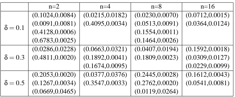
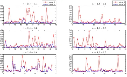
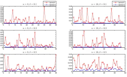
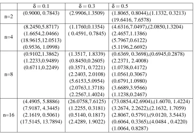
K when there is overfitting. We see that in either case, we

need to make use of the refinement relationship. We shall verify in the last section through extensive numerical simulations that the refinement kernel method is indeed able to provide an appropriate update of an operator-valued reproducing kernel when underfitting or overfitting occurs.

Before moving on to the characterization of refinement of operator-valued reproducing kernels, we collect here notations that will be frequently used in the rest of the paper. They will also be (or have been) defined when first used.

– X : a general input space,

– k · kΛ: the norm on a Hilbert or Banach spaceΛ,

–

W

: a Hilbert space, usually serving as the feature space of reproducing kernels,

–

L(

Λ): the space of bounded linear operators fromΛtoΛ,

–

L

+(Λ): the set of self-adjoint and positive bounded linear operators fromΛtoΛ,

–

L(

Λ,

W

): the space of bounded linear operators fromΛto

W

,

– K,G:

L(

Λ)-valued reproducing kernels,

–

H

K,

H

G: the RKHS of kernels K,G, respectively,

–

H

K

H

G: G is a refinement of K, namely,

H

K⊆

H

GandkfkHK =kfkHG for all f ∈

H

K,

– ˜X : the extended input space X_×Λ,

– ˜K: the scalar-valued kernel (11) associated with an

L(

Λ)-valued kernel K,

– µ,ν: scalar-valued or operator-valued measures,

– _|µ_|: the variation (19) of a measure µ,

– (Ω,

F

,µ): a measure space,

– µν: means that µ is the restriction ofνon some measurable set,

– L2(Ω,

B

,dµ): the Hilbert space (16) of square integrable

B

-valued functions on Ωwith re-spect to the measure µ,

– L2(Ω,dµ): the Hilbert space of scalar-valued square integrable functions onΩwith respect to the measure µ,

– L∞(Ω,dµ): the Banach space of essentially bounded measurable functions onΩwith respect to the measure µ,

– AB: see (29) for this refinement relation of two positive operators,

–

B(R

d_{,Λ): the set of all the}

_L

+(Λ)-valued measures of bounded variation on theσ-algebra of Borel subsets inRd_,

– γc,γs: the continuous part γc and singular partγs in the Lebesgue decomposition (38) of a

Borel measureγ,

– Lc,Ls: the continuous and singular parts (39) of a translation-invariant kernel,

– Λ_⊗

W

: the tensor product of two Hilbert spacesΛand

W

,

3. General Characterizations

The relationship between the RKHS of the sum of two operator-valued reproducing kernels and those of the summand kernels has been made clear in Theorem 1 on page 44 of Pedrick (1957). Our first characterization of refinement is a direct consequence of this result.

Proposition 1 Let K,G be two

L(

Λ)-valued reproducing kernels on X . Then

H

K

H

Gif and only

if G−K is an

L(

Λ)-valued reproducing kernel on X and

H

K∩

H

G−K={0}. If

H

K

H

Gthen

H

G−K

is the orthogonal complement of

H

K in

H

G.

Every reproducing kernel has a feature map representation. Specifically, K is an

L(

Λ)-valued reproducing kernel on X if and only if there exists a Hilbert space

W

and a mapping Φ: X _→

L(

Λ,

W

)such that

K(x,y) =Φ(y)∗Φ(x), x,y_∈X, (5)

where

L(

Λ,

W

)denotes the set of bounded linear operators fromΛto

W

, andΦ(y)∗_{is the adjoint} operator ofΦ(y). We callΦa feature map of K. The following lemma is useful in identifying the RKHS of a reproducing kernel given by a feature map representation (5).

Lemma 2 If K is an

L(

Λ)-valued reproducing kernel on X given by (5) then

H

K={Φ(·)∗u : u∈

W

}

with inner product

(Φ(_·)∗u,Φ(_·)∗v)_HK := (P_Φu,P_Φv)_W, u,v_∈

W

,

where PΦis the orthogonal projection of

W

onto

W

Φ:=span_{Φ(x)ξ: x_∈X,ξ_∈Λ_}.

The second characterization can be proved using Lemma 2 and the same arguments with those for the scalar-valued case (Xu and Zhang, 2007).

Theorem 3 Suppose that

L(

Λ)-valued reproducing kernels K and G are given by the feature maps

Φ: X_→

L(

Λ,

W

) andΦ′ : X_→

L(

Λ,

W

′_{), respectively. Assume that}

_W

_Φ=

_W

_and

_W

′

Φ′ =

W

′.

Then

H

K

H

Gif and only if there exists a bounded linear operator T from

W

′to

W

such that

TΦ′(x) =Φ(x)for all x_∈X,

and the adjoint operator T∗:

W

_→

W

′_{is isometric. In this case, G is a nontrivial refinement of K} if and only if T is not injective.

To illustrate the above useful results, we shall present a concrete example aiming at refining

L(

Λ)-valued reproducing kernels K with a finite-dimensional RKHS. A simple observation is made regarding such a kernel.

Proposition 4 AΛ-valued RKHS

H

Kis of finite dimension n∈Nif and only if there exists an n×n

hermitian and strictly positive-definite matrix A and n linearly independent functionsφj : X→Λ,

j_∈Nnsuch that

K(x,y)ξ= n

∑

j=1

n

∑

k=1

Proof Assume that

H

K is n dimensional with orthogonal basis{φj: j∈Nn}. As K(x,·)ξ∈

H

K for

all x_∈X ,ξ_∈Λ, there exist functions cj: X×Λ→Csuch that

K(x,y)ξ= n

∑

j=1

cj(ξ,x)φj(y), x,y∈X,ξ∈Λ.

Since_{φj: j∈Nn}is a basis for

H

K, each function f ∈

H

Khas the form

f= n

∑

j=1

djφj,dj∈C, j∈Nn.

Clearly, _kf_k:= (∑n_j=1|dj|2)1/2 is a norm on

H

K. It is equivalent to the original one on

H

K as

dim

H

K<∞. It is implied that there exists some C>0 such that

n

∑

j=1

|cj(ξ,x)|2≤CkK(x,·)ξk2_HK =C(K(x,x)ξ,ξ)Λ≤Ckξk2_ΛkK(x,x)k. (7)

Obviously, for each x_∈X and j_∈Nn, cj(·,x)is a linear functional on Λ. This together with (7)

implies that cj(·,x)are bounded linear functionals onΛ. By the Riesz representation theorem, there

existsψj: X →Λ,j∈Nnsuch that

cj(ξ,x) = (ξ,ψj(x))Λ.

We conclude that K has the form

K(x,y)ξ= n

∑

j=1

(ξ,ψj(x))Λφj(y), x,y∈X, ξ∈Λ. (8)

Since_{φj: j∈Nn}is an orthogonal basis for

H

K, by (3),

(ξ,ψj(x))Λ= (K(x,·)ξ,φj)HK= (ξ,φj(x))Λ,ξ∈Λ,x∈X.

It follows thatψj=φj, j∈Nn. Substituting this into (8) yields that

K(x,y)ξ= n

∑

j=1

(ξ,φj(x))Λφj(y), x,y∈X, ξ∈Λ,

which indeed is a special form of (6).

Conversely, assume that K has the form (6). We set

W

A:=IA2(Nn):={c= (cj: j∈Nn)∈Cn}

with inner product

(c,d)_I2

A(Nn):=

n

∑

j=1

n

∑

k=1

cjd¯kAjk.

IntroduceΦ: X_→

L(

Λ,

W

A)by settingΦ(x)ξ:= ((ξ,φj(x))Λ: j∈Nn). Direct computations show

that

Φ∗_(x)u=

∑

n

j=1

n

∑

k=1

Thus, we see that K(x,y) =Φ(y)∗_{Φ(x), x,y∈X , implying that K is an}

_L(

_{Λ)-valued reproducing} kernel. By the linear independence of φj, j∈Nn, span{Φ(x)ξ: x∈X,ξ∈Λ}=

W

A. We hence

apply Lemma 2 to get that

H

K={Φ(·)∗u : u∈

W

A}=span{φj: j∈Nn},

which is of dimension n.

By the above proposition, we let φj, j∈Nm be linearly independent functions from X to Λ,

where m_≥n are fixed positive integers. Let A and B be n_×n and m_×m hermitian and strictly positive-definite matrices, respectively. We define K by (6) in terms of matrix A and G by

G(x,y)ξ:= m

∑

j=1

m

∑

k=1

Bjk(ξ,φj(x))Λφk(y),x,y∈X (9)

and shall investigate conditions for G to be a refinement of K.

Proposition 5 Let K, G be defined by (6) and (9), respectively. Then

H

K

H

Gif and only if B−1is

an augmentation of A−1, namely, B−_jk1=A−_jk1, j,k∈Nn. In particular, if K, G have the form

K(x,y)ξ=

∑

j_∈Nn

aj(ξ,φj(x))Λφj(y),G(x,y)ξ=

∑

k_∈Nm

bk(ξ,φk(x))Λφk(y)

for some positive constants aj, bk, then

H

K

H

G if and only if aj =bj, j∈Nn. In both cases if

H

K

H

Gthen G is a nontrivial refinement of K if and only if m>n.

Proof It suffices to prove the first claim. We observe that K, G have the feature spaces

W

=I2

A(Nn)

and

W

′=I_B2(Nm), respectively, with feature maps

Φ(x)ξ:= ((ξ,φj(x))Λ: j∈Nn),Φ′(x)ξ:= ((ξ,φk(x))Λ: k∈Nm),x∈X,ξ∈Λ.

Suppose that

H

K

H

G, then by Theorem 3, there exists a bounded linear operator T :

W

′→

W

with properties as described there. It can be represented by an n_×m matrix D as

(TΦ′(x)ξ)j= m

∑

k=1

Djk(ξ,φk(x))Λ= (ξ,φj(x))Λ, x∈X,ξ∈Λ, (10)

which implies that D= [In,0], where Indenotes the n×n identity matrix. The adjoint operator T∗

of T is then represented by

T∗u=B−1

A 0

u,u_∈Cn_.

Since T∗is isometric, we get that

(T∗u,T∗v)_W′ = (u,v)_W,

which has the form

v∗[A,0]B−1BB−1

A 0

We derive from the above equation that

[A,0]B−1

A 0

=A.

Therefore, B−1is an augmentation of A−1. Conversely, if this is true then T :

W

′→

W

defined by Tu′:= [In,0]u′,u′∈Cm

satisfies the two properties in Theorem 3. As a result,

H

K

H

G.

It is worthwhile to point out that the above characterization is independent of the Hilbert space Λ.

Unlike the previous two characterizations, the third one comes as a surprise, telling us that theoretically we are able to reduce our consideration to the scalar-valued case.

Introduce for each

L

(Λ)-valued reproducing kernel K on X a scalar-valued reproducing kernel ˜

K on the extended input space ˜X :=X_×Λby setting

˜

K((x,ξ),(y,η)):= (K(x,y)ξ,η)Λ, x,y_∈X,ξ,η_∈Λ. (11)

By (1), ˜K is indeed positive-definite.

Proposition 6 There holds

H

K

H

G if and only if

H

K˜

H

_G˜. Furthermore, G is a nontrivial refinement of K on X if and only if ˜G is a nontrivial refinement of ˜K on ˜X .

Proof We first explore the close relationship between

H

K and

H

K˜. By (3), ˜

K((x,ξ),(y,η)) = (K(x,y)ξ,η)_Λ= (K(x,_·)ξ,K(y,_·)η)_HK,

which provides a natural feature mapΦ: ˜X_→

H

Kof ˜K

Φ((x,ξ)):=K(x,_·)ξ, x_∈X,ξ_∈Λ.

The density condition

W

Φ =

H

K is clearly satisfied by (3). We hence obtain by (2) that every

function ˜f in

H

K˜ is of the form ˜

f(x,ξ):= (f(x),ξ)_Λfor some f _∈

H

K

with

k_f˜_kH

˜

K=kfkHK.

Similar observations can be made about

H

_G˜.

It follows immediately that

H

_K˜

H

_G˜ if

H

K

H

G. On the other hand, suppose that

H

_K˜

H

_G˜. Then for each f _∈

H

Kthere exists some g∈

H

Gsuch that

(f(x),ξ)Λ= f˜(x,ξ) =g˜(x,ξ) = (g(x),ξ)Λfor all x_∈X, ξ_∈Λ (12)

and

kf_kHK =_kf˜_kH˜

Equation (12) implies that f =g. Therefore,

H

K

H

G.

It appears by Proposition 6 that we do not have to bother studying refinement of operator-valued reproducing kernels. Although the strategy sometimes does simplify the problem, the difficulty is generally not reduced significantly. Instead, the result might be viewed as transferring the complex-ity to the input space. Moreover, desirable properties such as translation invariance of the original kernels might be lost in the process. As a result, an independent study of the operator-valued case remains necessary and challenging.

4. Integral Representations

We shall characterize in this section the refinement of operator-valued kernels defined by two kinds of integral representations: the integral of operator-valued kernels with respect to a scalar-valued measure, and the integral of scalar-valued kernels with respect to an operator-valued measure. The characterizations to be established are crucial to the study of this paper as many useful operator-valued kernels are of an integral representation. Typical examples include the important translation-invariant operator-valued kernels and hessian kernels to be considered in the next section. We also point out in advance the difference in the refinement for the two kinds of integral represen-tations. Firstly, the first refinement corresponds to the same feature map and different measures, while the other when the Radon-Nikodym property is engaged has different feature maps and the same measure. The arguments of the proofs and the obtained results are essential different. The characterization of the first kind of refinement can be viewed as a straightforward generalization of that obtained in Xu and Zhang (2009), while the other one is mathematically nontrivial.

This section will be built on the theory of vector-valued measures and integrals (Berberian, 1966; Diestel and Uhl, 1977). Necessary preliminaries on the subjects will be explained in sufficient details.

4.1 Operator-valued Kernels With Respect to Scalar-valued Measures

Let us first introduce integration of a vector-valued function with respect to a scalar-valued measure. Let

F

be a σ-algebra of subsets of a fixed setΩ, µ a finite nonnegative measure on

F

, and

B

a Banach space. We are concerned with

B

-valued functions onΩ. A function f :Ω_→

B

is said to be simple if

f = n

∑

j=1

ajχEj (13)

for some finitely many aj∈

B

and pairwise disjoint subsets Ej∈

F

, j∈Nn. A function f :Ω→

B

is called µ-measurable if there exists a sequence of

B

-valued simple functions fnonΩsuch that

lim

n→∞kfn(t)−f(t)kB =0 for µ−a.e. t∈Ω,

where µ₋a.e. stands for “everywhere except for a set of zero µ measure”. Finally, a

B

-valued function f onΩis called µ-Bochner integrable if there exists a sequence of simple functions fn: Ω→

B

such that

lim

n→∞

Z

The integral of a simple function f of the form (13) on any E∈

F

with respect to µ is defined by

Z

E

f dµ := n

∑

j=1

ajµ(Ej∩E).

In general, suppose that f is a µ-Bochner integrable function fromΩto

B

, that is, (14) holds true. Then it is obvious that for each E_∈

F

,R_E fndµ, n∈Nform a Cauchy sequence in

B

. Therefore,

Z

E f dµ : = lim

n_→∞ Z

E fndµ

.

The resulting integralR_E f dµ is an element in

B

.

It is known that a µ-measurable function f :Ω_→

B

is Bochner integrable if and only if

Z

Ωkf(t)kBdµ(t)<+∞.

This provides a way for us to comprehend the integralR_E f dµ in the most needed case when f is

L(

Λ)-valued. If

B

=

L(

Λ)then we have for each E_∈

F

that

Z

E

f dµξ,η

Λ= Z

E

(f(t)ξ,η)_Λdµ(t), ξ,η_∈Λ. (15)

Clearly, the right hand side above defines a sesquilinear form onΛ_×Λwhich is bounded as

Z

E

(f(t)ξ,η)Λdµ(t)

≤

Z

Ek

f(t)_kL(Λ)dµ(t)kξkΛkηkΛ,

where_{k · kL(Λ)}is the operator norm on

L(

Λ). As a result, (15) gives an equivalent way of defining the integralR_E f dµ as a bounded linear operator onΛ(Conway, 1990).

We introduce another notation before returning to reproducing kernels. Denote by L2(Ω,

B

,dµ)

the Banach space of all the µ-measurable functions f :Ω_→

B

such that

kf_kL2_(Ω,B,dµ):=

Z

Ωkf(t)k

2 Bdµ(t)

1/2

<+∞. (16)

When

B

=C, L2(Ω,C,dµ)will be abbreviated as L2(Ω,dµ). When

B

is a Hilbert space, L2(Ω,

B

,dµ)

is also a Hilbert space with the inner product

(f,g)L2₍Ω_,B,dµ):= Z

Ω(f(t),g(t))Bdµ(t), f,g∈L

2_(Ω,

_B

_,dµ). The discussion in this section by far can be found in Diestel and Uhl (1977).

Let µ,ν be two finite nonnegative measures on a σ-algebra

F

of subsets of Ω. To intro-duce our

L(

Λ)-valued reproducing kernels, we also let

W

be a Hilbert space and φa mapping from X_×Ωto

L(

Λ,

W

)such that for each x_∈X ,φ(x,_·)belongs to both L2(Ω,

L(

Λ,

W

),dµ)and L2(Ω,

L(

Λ,

W

),dν). We shall investigate conditions that ensure

H

K

H

Gwhere

K(x,y) = Z

Ωφ(y,t)

and

G(x,y) = Z

Ωφ(y,t)

∗_{φ(x,t)dν(t), x,y∈X, (18)}

whereφ(y,t)∗ is the adjoint operator ofφ(y,t). Note that K,G are well-defined as the integrand is Bochner integrable with respect to both µ andν. For instance, we observe by the Cauchy-Schwartz inequality for all x,y_∈X that

Z

Ωkφ(y,t)

∗_φ(x,t)k

L(Λ)dµ(t) ≤

Z

Ωkφ(y,t)

∗_k

L(W,Λ)kφ(x,t)kL(Λ,W)dµ(t)

= Z

Ωkφ(y,t)kL(Λ,W)kφ(x,t)kL(Λ,W)dµ(t)

≤ kφ(y,_·)_kL2₍Ω_,L(Λ_,W),dµ)kφ(x,·)k_L2₍Ω_,L(Λ_,W),dµ).

An alternative of expressing K,G is for all x,y_∈X ,ξ,η_∈Λthat

˜

K((x,ξ),(y,η)) = (K(x,y)ξ,η)_Λ= Z

Ω(φ(x,t)ξ,φ(y,t)η)Wdµ(t)

and

˜

G((x,ξ),(y,η)) = (G(x,y)ξ,η)Λ= Z

Ω(φ(x,t)ξ,φ(y,t)η)Wdν(t).

When Λ=

W

=C, a characterization of

H

K

H

G in terms of µ,νhas been established in

Xu and Zhang (2009). The relation, between the two measures, which we shall need is absolute continuity. We say that µ is absolutely continuous with respect to νif for all E _∈

F

, ν(E) =0 implies µ(E) =0. In this case, by the Radon-Nikodym theorem (see, Rudin, 1987, page 121) for scalar-valued measures, there exists a nonnegativeν-integrable function, denoted by dµ/dν, such that

µ(E) = Z

E

dµ

dν(t)dν(t)for all E∈

F

.

We write µνif µ is absolutely continuous with respect toνand dµ/dν_{∈ {}0,1_}ν₋a.e. Thus, µνif and only if µ is the restriction ofνon some measurable set in

F

.

WhenΛ=

W

=C, it was proved in Theorem 8 of Xu and Zhang (2009) that if span_{φ(x,_·): x_∈X_}is dense in both L2(Ω,dµ)and L2(Ω,dν)then G is a refinement of K if and only if µν. If µνthen G is a nontrivial refinement of K if and only ifν(Ω)>µ(Ω).

Theorem 7 Let K,G be given by (17) and (18). If span_{φ(x,_·)ξ: x_∈X, ξ_∈Λ_}is dense in both L2(Ω,

W

,dµ)and L2(Ω,

W

,dν)then

H

K

H

Gif and only if µν. In this case, the refinement G

of K is nontrivial if and only ifν(Ω)₋µ(Ω)>0.

4.2 Scalar-valued Kernels with Respect to Operator-valued Measures

Again,

B

is a Banach space and

F

denotes aσ-algebra consisting of subsets of a fixed setΩ. A

B

-valued measure on

F

is a function from

F

to

B

that is countably additive in the sense that for every sequence of pairwise disjoint sets Ej∈

F

, j∈N

µ

[∞

j=1 Ej

= ∞

∑

j=1

µ(Ej),

where the series converges in the norm of

B

. Every

B

-valued measure µ on

F

comes with a scalar-valued measure_|µ_|on

F

defined by

|µ_|(E):=sup P F

∑

_∈P

kµ(F)_kB, E∈

F

, (19)

where the supremum is taken over all partitions

P

of E into countably many pairwise disjoint mem-bers of

F

. We call _|µ_|the variation of µ and shall only work with these vector-valued measures µ that are of bounded variation, that is,_|µ_|(Ω)<+∞. We note that µ vanishes on sets of zero_|µ_| measure. It implies that µ is absolutely continuous with respect to_|µ_|in the sense that

lim

|µ(E)|→0µ(E) =0.

The only type of integration that we shall need is to integrate a bounded

F

-measurable scalar-valued function with respect to a

B

-valued measure of bounded variation. Denote by L∞(Ω,d_|µ_|)

the Banach space of essentially bounded

F

-measurable functions onΩwith the norm

kf_kL∞(Ω,d|µ|):=inf{a≥0 :|µ|({|f|>a}) =0}. For a simple function f :Ω_→Cof the form

f = n

∑

j=1

αjχEj,

whereαj∈Cand Ej are pairwise disjoint members in

F

, we define Z

E

f dµ := n

∑

j=1

αjµ(Ej∩E), E∈

F

.

Clearly,

Z

E

f dµ

B≤ k

f_kL∞(Ω,d|µ|)|µ|(E).

Therefore, the map sending a simple function f toR_E f dµ can be uniquely extended to a bounded linear operator from L∞(Ω,d_|µ_|)to

B

. The outcome of the application of the resulting operator on a general f _∈L∞(Ω,d_|µ_|)is still denoted byR_E f dµ. This is how the

B

-valued integral is defined.

It is time to present the second type of reproducing kernels defined by integration:

K(x,y):= Z

ΩΨ(x,y,t)dµ(t), x,y∈X, (20)

where µ is an

L

+(Λ)-valued measure on

F

of bounded variation, andΨ is a scalar-valued func-tion such thatΨ(_·,_·,t)is a scalar-valued reproducing kernel on X for all t_∈Ωand for all x,y_∈X ,

Proposition 8 With the above assumptions onΨand µ, the function K defined by (20) is an

L(

Λ) -valued reproducing kernel on X .

Proof Fix finite xj∈X andξj∈Λ, j∈Nn. For anyε>0, there exist simple functions

fj,k:= m

∑

l=1

αj,k,lχEl, j,k∈Nn

such that

kΨ(xj,xk,·)−fj,kkL∞(Ω,d|µ|)<ε, j,k∈Nn. (21)

Here,αj,k,l ∈Cand El are pairwise disjoint sets in

F

with |µ|(El)>0, l ∈Nm. By (21) and the

definition of integration in this section,

n

∑

j=1

n

∑

k=1

(K(xj,xk)ξj,ξk)Λ− n

∑

j=1

n

∑

k=1

Z

Ωfj,kdµ

ξj,ξk Λ

≤ε|µ_|(Ω)

n

∑

j=1

kξjkΛ 2

. (22)

We may choose by (21) for each l_∈Nmsome tl∈El such that

Ψ(x_j,x_k,t_l)−α_j,k,l ≤ε.

Letting

S := n

∑

j=1

n

∑

k=1

m

∑

l=1

Ψ(xj,xk,tl)(µ(El)ξj,ξk)Λ,

we get by the above equation that

n

∑

j=1

n

∑

k=1

Z

Ωfj,kdµ

ξj,ξk

Λ−S ≤ n

∑

j=1

n

∑

k=1

m

∑

l=1

|αj,k,l−Ψ(xj,xk,tl)|(µ(El)ξj,ξk)Λ ≤ε n

∑

j=1

n

∑

k=1

m

∑

l=1

kµ(El)kL(Λ)kξjkΛkξkkΛ≤ε|µ|(Ω)

n

∑

j=1

kξjkΛ 2

. (23)

Combining (22) and (23) yields that

n

∑

j=1

n

∑

k=1

(K(xj,xk)ξj,ξk)Λ−S

≤2ε_|µ_|(Ω)

n

∑

j=1

kξjkΛ 2

. (24)

Since Ψ(_·,_·,tl) is a scalar-valued reproducing kernel on X , [Ψ(xj,xk,tl): j,k∈Nn] is a positive

semi-definite matrix for each l_∈Nm. So are[(µ(El)ξj,ξk)Λ: j,k∈Nn], l∈Nmas µ(El)∈

L

+(Λ). By the Schur product theorem (see, for example, Horn and Johnson, 1991, page 309), the Hadamard product of two positive semi-definite matrices remains positive semi-definite. We obtain by this fact that S>0, which together with (24), and the fact thatεcan be arbitrarily small, proves (1).

To investigate the refinement relationship, we shall consider a simplified version of (20) that covers a large class of operator-valued reproducing kernels. Letφ: X_×Ω_→Cbe such thatφ(x,_·)

is a bounded

F

-measurable function for every x_∈X and such that

We shall see by the concrete examples in the next section that the denseness requirement (25) is not too restricted in applications. The kernels we shall consider are

K(x,y):= Z

Ωφ(x,t)φ(y,t)dµ(t), x,y∈X (26)

and

G(x,y):= Z

Ωφ(x,t)φ(y,t)dν(t), x,y∈X, (27)

where µ,ν are two

L

+(Λ)-valued measures on

F

of bounded variation. By Proposition 8, K,G are

L(

Λ)-valued reproducing kernels on X . Our idea is to use the Radon-Nikodym property of vector-valued measures to study the refinement property.

Let

B

be a Banach space andγ a finite nonnegative measure on

F

. We say that a

B

-valued measureρon

F

of bounded variation has the Radon-Nikodym property with respect toγif there is aγ-Bochner integrable functionΓ:Ω_→

L

+(Λ)such that for all E∈

F

ρ(E) = Z

EΓ

dγ.

Apparently, this could only be true whenρis absolutely continuous with respect toγ. For this reason, we also say that the space

B

has the Radon-Nikodym property with respect toγif every

B

-valued measure of bounded variation that is absolutely continuous with respect toγhas the Radon-Nikodym property with respect toγ. Moreover,

B

is said to have the Radon-Nikodym property if it has it with respect to any finite nonnegative measure on any measure space

F

.

Strikingly different from the scalar-valued case, a Banach space

B

may not have the Radon-Nikodym property. For instance, the Banach space c0of all sequencesα:= (αj∈C: j∈N)with

lim

j→∞|αj|=0

under the norm_kα_kc0:=sup{|αj|: j∈N}does not have the property with respect to the Lebesgue

measure (see, Diestel and Uhl, 1977, page 60). Consequently, the space

L(

Λ) does not have the Radon-Nikodym property whenΛis infinite-dimensional. To see this, sinceΛis separable we let

{ej: j∈N}be an orthonormal basis forΛ. Denote by

L

0(Λ)the set of all the operators T∈

L(

Λ) such that

Tej=αjej, j∈N

for someα∈c0. One sees thatkTkL(Λ)=kαkc0 (Conway, 1990). As a result,

L

0(Λ)is a closed

subspace of

L(

Λ)that is isometrically isomorphic to c0. Since c0does not have the Radon-Nikodym property, neither does

L

0(Λ). A Banach space has the Radon-Nikodym property if and only if each of its closed linear subspaces does (Diestel and Uhl, 1977). By this fact,

L

(Λ)does not have Radon-Nikodym property.

Solomjak, 1987). Denote for each compact operator T ∈

L(

Λ) by sj(T), j∈N, the nonnegative

square root of the j-th largest eigenvalue of T∗T . It is called the j-th singular number of T . For p_∈(1,+∞), the p-th Schatten class

S

p(Λ) consists of all the compact linear operators T ∈

L(

Λ)

with the norm

kT_kSp(Λ):=

∞

∑

j=1

(sj(T))p 1/p

<+∞.

The p-th Schatten class Sp(Λ)is a reflexive Banach space and hence has the Radon-Nikodym

prop-erty. When p=2, S2(Λ)is the class of Hilbert-Schmidt operators and

kT_kS2(Λ)=

∞

∑

j=1

kTejkΛ 1/2

.

We shall not go into further details about the Radon-Nikodym property. Interested readers are referred to Chapter III of Diestel and Uhl (1977) and the references therein.

The assumption we shall need is that there exists a finite nonnegative measure γon

F

such that both µ andνhave the Radon-Nikodym property with respect toγ. In other words, there exist γ-Bochner integrable functionsΓµ,Γν:Ω→

L

+(Λ)such that

µ(E) = Z

E

Γµdγ and ν(E) = Z

E

Γνdγ for all E_∈

F

. (28)

Such two functions exist if γ:=_|µ_|+_|ν_|and µ,νtake values in the p-th Schatten class of

L(

Λ), 1<p<+∞.

Suppose that K,G are given by (26) and (27), whereφ,µ,νsatisfy (25) and (28). Our purpose is to investigate

H

K

H

G. To this end, let us first identify

H

K˜ and

H

G˜. We shall only present results for

H

K˜ as those for

H

_G˜ have a similar form.

Lemma 9 The RKHS

H

_K˜ consists of functions Ff of the form

Ff(x,ξ):= Z

Ω(Γµ(t)f(t),ξ)Λφ(x,t)dγ(t), x∈X, ξ∈Λ,

where f can be an arbitrary element from the Hilbert space

W

µofγ-measurable functions fromΩ

toΛsuch that

kf_kWµ :=

Z

Ω(Γµ(t)f(t),f(t))Λdγ(t) 1/2

<+∞.

Moreover,_kFfkHK˜ =kfkWµ for all f ∈

W

µ.

Proof We observe for all x,y_∈X andξ,η_∈Λthat ˜

K((x,ξ),(y,η)) = Z

Ωφ(x,t)φ(y,t)(Γµ(t)ξ,η)Λdγ(t).

Thus, we may choose

W

µas a feature space for ˜K. The associated feature mapΦµ: X×Λ→

W

µis

then selected as

We next verify the denseness condition that span{Φµ(x,ξ): x∈X, ξ∈Λ}=

W

µ. Suppose that

f _∈

W

µis orthogonal toΦµ(x,ξ)for all x∈X andξ∈Λ, that is, Z

Ω(Γµf(t),ξ)Λφ(x,t)dγ(t) =0 for all x∈X, ξ∈Λ.

By (25),

(Γµ(t)f(t),ξ)Λ=0γ−a.e.

As this holds for an arbitraryξ_∈Λ, Γµ(t)f(t) =0γ−a.e. It implies that kfkWµ =0. The result

now follows immediately from Lemma 2.

For two operators A,B_∈

L

+(Λ), we write AB if for allξ∈Λthere exists someη∈Λsuch that

Aξ=Bηand(Aξ,ξ)_Λ= (Bη,η)_Λ. (29)

We make a simple observation about this special relationship between two linear operators.

Let ker(A)and ran(A)be the kernel and range of A, respectively. If ran(A)is closed then as A is self-adjoint, there holds the direct sum decomposition

Λ=ker(A)_⊕ran(A). (30)

Thus, A is bijective and bounded from ran(A)to ran(A). By the open mapping theorem, it has a bounded inverse on ran(A), which we denote by A−1.

Proposition 10 Suppose that A,B_∈

L

+(Λ)have closed range. Then AB if and only if

ran(A)_⊆ran(B) (31)

and

PB,AB−1=A−1on ran(A), (32)

where PB,Adenotes the orthogonal projection from ran(B)to ran(A). Particularly, if A is onto then

AB if and only if A=B.

Proof Let A,B have closed range. Suppose first that AB. Then (31) clearly holds true. Set for eachξ_∈ran(A)

η_ξ:=B−1Aξ.

Clearly, the mappingξ→ηξis linear from ran(A)to ran(B). Thus, we have for arbitraryξ,ξ′_∈Λ that

(Aξ′+Aξ,ξ′+ξ)_Λ= (Bη_ξ′_+ξ,η_ξ′_+ξ)_Λ= (Bη_ξ′+Bη_ξ,η_ξ′+η_ξ)_Λ,

which implies that

Re(Aξ′,ξ)_Λ= Re(Bη_ξ′,η_ξ)Λ.

A textbook trick yields that for allξ,ξ′_∈ran(A),

We hence obtain thatξ−ηξ∈ker(A)for allξ∈ran(A). Consequently,

Aξ₋AB−1Aξ=Aξ₋Aη_ξ=0 for allξ_∈ran(A), from which (32) follows.

On the other hand, suppose that (31) and (32) hold true. Then we choose for eachξ∈Λ

η:=B−1Aξ and verify that Bη=Aξand

(Bη,η)Λ= (Aξ,B−1Aξ)Λ= (Aξ,PB,AB−1Aξ)Λ= (Aξ,A−1Aξ)Λ= (Aξ,ξ)Λ.

Finally, if A is onto then by (31), ran(A) =ran(B) =Λ. According to (30), both A and B are in-jective. Therefore, they possess a bounded inverse onΛ. It implies that PB,Ais the identity operator

onΛ. By Equation (32), A=B. The proof is complete.

We are ready to present the main result of this section.

Theorem 11 Let K,G be given by (26) and (27), whereφ,µ,νsatisfy (25) and (28). Then

H

K

H

G

if and only ifΓµΓνγ−a.e.

Proof By Proposition 6 and Lemma 9,

H

K

H

Gif and only if for all f ∈

W

µ, there exists some

g_∈

W

νsuch that

Z

Ω(Γµ(t)f(t),ξ)Λφ(x,t)dγ(t) = Z

Ω(Γν(t)g(t),ξ)Λφ(x,t)dγ(t)for all x∈X,ξ∈Λ (33)

and _Z

Ω(Γµ(t)f(t),f(t))Λdγ(t) = Z

Ω(Γν(t)g(t),g(t))Λdγ(t). (34)

By the denseness condition (25), (33) holds true if and only if

(Γµ(t)f(t),ξ)Λ= (Γν(t)g(t),ξ)Λ forγ−a.e. t∈Ωand allξ∈Λ,

which is equivalent to

Γµ(t)f(t) =Γν(t)g(t)forγ−a.e. t∈Ω. (35)

We conclude that

H

K

H

Gif and only if for every f ∈

W

µ, there exists some g∈

W

ν such that

Equations (34) and (35) hold true.

Suppose thatΓµΓνγ−a.e. Then clearly, for each f ∈

W

µ, we can find a function g :Ω→Λ

which is definedγ-almost everywhere and satisfies (35) and

(Γµ(t)f(t),f(t))Λ= (Γν(t)g(t),g(t))Λforγ−a.e. t∈Ω.

The above equation implies (34). Therefore,

H

K

H

G.

On the other hand, suppose that we can find for every f _∈

W

µsome gf ∈

W

νsatisfying (34) and

(35). The function gf can be chosen so that f →gf is linear from

W

µto

W

ν. A trick similar to that

used in Lemma 9 enables us to obtain from (34) and (35) that

Z

Ω(Γµ(t)f

′_(t),f(t)−g

Letting f′:=φ(x,_·)ξfor arbitrary x∈X andξ∈Λin the above equation and invoking (25), we have that

Γµ(t)(f(t)−gf(t)) =0 forγ−a.e. t∈Ω.

By the above equation and (35), we get forγ-almost every t_∈Ωthat

(Γν(t)gf(t),gf(t))Λ= (Γµ(t)f(t),gf(t))Λ= (f(t),Γµ(t)gf(t))Λ= (f(t),Γµ(t)f(t))Λ= (Γµ(t)f(t),f(t))Λ.

Since (35) and the above equation are true for an arbitrary f _∈

W

µ,ΓµΓνγ−a.e.

5. Examples

We present in this section several concrete examples of refinement of operator-valued reproducing kernels. They are built on the general characterizations established in the last two sections.

5.1 Translation Invariant Reproducing Kernels

Let d_∈Nand K be an

L(

Λ)-valued reproducing kernel onRd_{. We say that K is translation invariant}

if for all x,y,a_∈Rd

K(x₋a,y₋a) =K(x,y).

A celebrated characterization due to Bochner (1959) states that every continuous scalar-valued translation invariant reproducing kernel on Rd _{must be the Fourier transform of a finite}

nonneg-ative Borel measure onRd_{, and vice versa. This result has been generalized to the operator-valued}

case (Berberian, 1966; Carmeli et al., 2010; Fillmore, 1970). Specifically, a continuous function K fromRd_×Rd _to

_L(

Λ_{)is a translation invariant reproducing kernel if and only if it has the form}

K(x,y) = Z

Rde

i(x−y)·t_{dµ(t), x,y}

∈Rd_{, (36)}

for some µ_∈

B(R

d_{,Λ), the set of all the}

_L

+(Λ)-valued measures of bounded variation on the σ -algebra of Borel subsets inRd_{. Let G be the kernel given by}

G(x,y) = Z

Rde

i(x−y)·t_{dν(t), x,y}

∈Rd_{, (37)}

whereν_∈

B(R

d_{,Λ). The purpose of this subsection is to characterize}

_H

K

H

Gin terms of µ,ν.

To this end, we first investigate the structure of the RKHS of a translation invariant

L(

Λ)-valued reproducing kernel.

Letγbe an arbitrary measure in

B(R

d_,Λ_{)and L the associated translation invariant reproducing}

kernel defined by

L(x,y) = Z

Rde

i(x−y)·t_{dγ(t), x,y}

∈Rd_.

There exists a decomposition ofγwith respect to the Lebesgue measure dx onRd_{(Diestel and Uhl,}

1977) as follows:

whereγc,γsare the unique measures in

B

(Rd,Λ)such thatγcis absolutely continuous with respect

to dx, and for each continuous linear functionalλon

L(

Λ), the scalar-valued measureλγsand dx

are mutually singular. It follows from this decomposition of measures a decomposition of L:

L=Lc+Ls,

where

Lc(x,y) = Z

Rde

i(x₋y)·t_dγ

c(t), Ls(x,y) = Z

Rde

i(x₋y)·t_dγ

s(t), x,y∈Rd. (39)

Our first observation is that

H

Lis the orthogonal direct sum of

H

Lcand

H

Ls. Two lemmas are needed

to prove this useful fact.

Lemma 12 Let Lc,Lsbe given by (39). Then for allξ∈Λand x,y∈Rd (La(x,y)ξ,ξ)Λ=

Z

Rde

i(x−y)·t_dγ

a,ξ(t), a=c or s, (40)

whereγa,ξis a scalar-valued Borel measure onRd defined for each Borel set E⊆Rd by

γa,ξ(E):= (γa(E)ξ,ξ)Λ, a=c or s.

Proof Let a_{∈ {}c,s_},ξ_∈Λ, x,y_∈Rd_{, and s}

nbe a sequence of simple functions onRdthat converges

to ei(x−y)·t in L∞(Rd_{,dx). Then}

lim

n_→∞

Z

Rdsndγa

ξ,ξ

Λ= (La(x,y)ξ,ξ)Λ.

By definition, we have for each n_∈Nthat

lim

n→∞

Z

Rdsndγa

ξ,ξ

Λ =

Z

Rdsndγa,ξ.

As

lim

n_→∞ Z

Rdsndγa,ξ=

Z

Rde

i(x−y)·t_dγ a,ξ(t),

we conclude from the previous two equations that (40) holds true.

Lemma 13 There holds

H

Lc∩

H

Ls={0}.

Proof We introduce for eachξ_∈Λtwo scalar-valued translation invariant reproducing kernels on

Rd_{by setting}

Aa(x,y):= (La(x,y)ξ,ξ)Λ, x,y∈Rd, a∈ {c,s}.

By Lemma 12, we have the alternative representations for Acand As

Aa(x,y) = Z

Rde

i(x−y)·t_dγ

By the Lebesgue decomposition of γ, γc,ξ is absolutely continuous with respect to dx while γs,ξ

and dx are mutually singular. As a consequence,

H

Ac∩

H

As ={0}by Lemma 17 in Xu and Zhang

(2009).

Let a_{∈ {}c,s_}. By (3),

Aa(x,y) = (La(x,·)ξ,La(y,·)ξ)HLa, x,y∈R

d_.

A feature map for Aamay hence be chosen as

Φa(x):=La(x,·)ξ, x∈Rd

with the feature space being

H

La. We identify by Lemma 2 that

H

Aa={(f˜(·),ξ)Λ: ˜f ∈

H

La}. (41)

Assume that

H

Lc∩

H

Ls6={0}. Then there exist nontrivial functions ˜f ∈

H

Lc and ˜g∈

H

Ls such

that ˜f =g. As a result, there exists some˜ ξ_∈Λ such that(_f˜_{(·),ξ)Λis not the trivial function. By} equation (41)

(_f˜_{(·),ξ)Λ= (g˜(·),ξ)Λ∈}

_H

_A

c∩

H

As,

contradicting the fact that

H

Ac∩

H

As ={0}.

Theorem 14 The space

H

Lis the orthogonal direct sum of

H

Lcand

H

Ls, namely,

H

L=

H

Lc

L

H

Ls.

Proof The result follows directly from Lemma 13 and Proposition 1.

We are now in a position to study the refinement relationship

H

K

H

G, where K,G are defined

by (36) and (37). Firstly, the task can be separated into two related ones according to the Lebesgue decomposition of measures µ,ν.

Proposition 15 There holds

H

K

H

Gif and only if

H

Kc

H

Gc and

H

Ks

H

Gs.

Proof By Theorem 14,

H

K =

H

Kc

L

H

Ks and

H

G=

H

Gc

L

H

Gs. Therefore, if

H

Kc

H

Gc and

H

Ks

H

Gs then

H

K

H

G.

On the other hand, suppose that

H

K

H

G. Let f ∈

H

Kc. Then f ∈

H

K andkfkH_Kc =kfkHK.

Since

H

K

H

G, there exists g∈

H

Gcand h∈

H

Gs such that

f =g+h

and

kf_k2_H

Kc =kfk

2

HK =kg+hk

2

HG =kgk

2

HGc+khk

2 HGs.

Therefore, to show that

H

Kc

H

Gc it suffices to show that h=0. Assume that h6=0. Note that

f₋g_∈

H

Kc+Gc(Pedrick, 1957), we get that