Sub-Local Constraint-Based Learning of Bayesian Networks Using A
Joint Dependence Criterion
Rami Mahdi [email protected]
Department of Genetic Medicine Weill Cornell Medical College New York, NY, 10065, USA
Jason Mezey [email protected]
Department of Biological Statistics and Computational Biology Cornell University
Ithaca, NY, 14853, USA
Editor:Peter Spirtes
Abstract
Constraint-based learning of Bayesian networks (BN) from limited data can lead to multiple testing problems when recovering dense areas of the skeleton and to conflicting results in the orientation of edges. In this paper, we present a new constraint-based algorithm, light mutual min (LMM) for improved accuracy of BN learning from small sample data. LMM improves the assessment of can-didate edges by using a ranking criterion that considers conditional independence on neighboring variables at both sides of an edge simultaneously. The algorithm also employs an adaptive relax-ation of constraints that, selectively, allows some nodes not to condition on some neighbors. This relaxation aims at reducing the incorrect rejection of true edges connecting high degree nodes due to multiple testing. LMM additionally incorporates a new criterion for ranking v-structures that is used to recover the completed partially directed acyclic graph (CPDAG) and to resolve conflicting v-structures, a common problem in small sample constraint-based learning. Using simulated data, each of these components of LMM is shown to significantly improve network inference compared to commonly applied methods when learning from limited data, including more accurate recovery of skeletons and CPDAGs compared to the PC, MaxMin, and MaxMin hill climbing algorithms. A proof of asymptotic correctness is also provided for LMM for recovering the correct skeleton and CPDAG.
Keywords: Bayesian networks, skeleton, constraint-based learning, mutual min
1. Introduction
Learning a Bayesian network (BN) from observational data is a reverse engineering process that can provide insight into the direct relations between observed variables and can be used to establish causation (Pearl, 1988; Spirtes et al., 2001). BNs have been used in learning applications in a num-ber of fields including systems biology (Friedman et al., 2000; Friedman, 2004), medicine (Cowell et al., 1999), and artificial intelligence (Russell and Norvig, 2009) where emerging applications and the growing availability of complex data sets containing thousands of variables are requiring faster, more scalable, and more accurate methods.
is super exponential in the number of variables being modeled, an exhaustive search is not possible for more than a few tens of variables (Chickering et al., 2004) while heuristic search methods tend to converge to suboptimal solutions. This scalability issue is a known limitation of score-based methods, where a scoring criterion such as the Bayesian information criterion (BIC) (Cooper and Herskovits, 1992) or the minimum description length criterion (MDL) (Lam and Bacchus, 1994) is used to rank candidate networks.
An alternative learning approach to score-based search is the use of conditional independence testing, also referred to as constraint-based learning. Methods in this class such as the IC algorithm (inductive causation) (Pearl, 1988), PC algorithm (Spirtes et al., 2001), and TPDA algorithm (three-phase dependency analysis) (Cheng et al., 2002), first recover the skeleton of the network and edges are oriented afterward. The learning is performed in a way to ensure that the resulting network is consistent with the conditional independences/dependencies entailed by the observations. Under the faithfulness assumption (see Section 3 for definition), constraint-based methods were shown to recover the correct network as the size of the observed samples approaches infinity (Zhang and Spirtes, 2003; Kalisch and B¨uhlmann, 2007). Moreover, their computational complexity has a poly-nomial order when the maximum number of connections per node is bounded. Constraint-based methods have also been used in combination with score-based search in what typically is referred to as hybrid learning. Hybrid methods such as the SC algorithm (sparse candidate) (Friedman et al., 1999), MMHC algorithm (MaxMin hill climbing) (Tsamardinos et al., 2006), and the COS algo-rithm (constrained optimal search) (Perrier et al., 2008) first recover a super structure of the skeleton using a constraint-based approach. Afterward, a constrained score-based search is used to find an optimal network where the search is restricted only to edges existing in the super structure. This strategy can reduce the size of the search space considerably and can lead to higher score solutions. Although constraint-based learning can, under appropriate assumptions, recover the correct graph in the asymptotic limit, its performance in real applications depends heavily on the accuracy of independence testing, which in turn is sensitive to noise and sample size. As will be discussed in this paper, when learning from small sample data, the use of conditional independence testing can lead to multiple testing problems that deteriorate the accuracy of skeleton recovery and to conflict-ing results in the orientation of edges. In addition, errors in the first phase of recoverconflict-ing the skeleton can also deteriorate the precision of orienting the edges, resulting in a propagated error.
2. Contribution
Moreover, we present a new approach to recover v-structures in a given skeleton based on the level of induced dependence caused by common neighbors, and LMM is extended to recover the completed partially directed acyclic graph (CPDAG) of the equivalence class. The name light mu-tual min is motivated by the fact that the algorithm is fast and uses reduced sets of neighbors (light) in addition to ranking edges using a measure that combines the minimal dependence from both sides of an edge (mutual min). Also, we refer to LMM as a sub-local approach due to using reduced sets of neighbors for independence testing as compared to local algorithms such as the PC and MaxMin algorithms which use subsets of all neighbors for conditional independence testing.
For completeness, a proof of asymptotic correctness is provided to show that the proposed ap-proaches will recover the correct skeleton and CPDAG when the number of observations grows suf-ficiently large. Also, to empirically assess performance, we compare LMM to the PC and MaxMin algorithms, two of the most popular and computationally efficient BN learning methods (Spirtes et al., 2001; Tsamardinos et al., 2006; Kalisch et al., 2010). Based on empirical evaluation us-ing simulated data, LMM is shown to significantly and consistently outperform both the PC and MaxMin algorithms in recovering the skeleton of the graph in terms of both accuracy and speed when learning from limited sample data. In addition, the extended LMM is found to recover more accurate CPDAGs than the PC algorithm, while being competitive with the MMHC algorithm in the small network case and more accurate in the large network case.
The rest of this paper is organized as follows: Section 3 presents necessary definitions. Section 4 presents related work. Section 5 presents a discussion of the limitations of existing methods. Section 6 presents our proposed methods. Section 7 presents experimental results and comparison to other methods. A proof of asymptotic correctness for the presented methods is provided in the Appendix for the recovery of both the skeleton and the CPDAG.
Availability: Our implementation of all presented methods in addition to a supplementary
material of further discussion and illustrations are made available with this publication and they also can be accessed athttp://www.mloss.org/software/view/460/or alternatively athttp: //mezeysoftware.bscb.cornell.edu/index.php/LMM.
3. Definitions and Preliminaries
In this section, we present necessary definitions and notations following Pearl (1988) and Neapolitan (2004) with slight variations.
Definition 1 (Directed Graph) A directed graph G= (V,E)consists of a set of nodes representing variables V ={1, ...,p}and a set of edges E⊆V×V where an edge(i,j)∈E implies that E(i,j)
is an edge pointing from Vi (parent) to Vj (child). Two variables i and j are adjacent in G if and
only if(i,j)∈E or(j,i)∈E.
In this paper, the notationCPi∗is used to refer to the true set of child and parent variables of the variableiwhile the notationCPi is used to refer to the set of child and parent variables ofithat are
being inferred by the algorithm. The set of child and parent variables are also sometimes referred to as the neighbor set ofi.
Definition 2 (Directed Acyclic Graph (DAG)) A directed graph G= (V,E) is said to be acyclic if and only if for every node Vi in the graph, there does not exist a path of connected and directed
edges such that starting from node Viand following the direction of edges can lead back to the same
Definition 3 (Skeleton) The skeleton of a directed graph G= (V,E) is a graph that contains all the nodes and edges of G such that all the edges have no directions. Every undirected edge in the skeleton represents a parent-child relation without informing who is the parent and who is the child.
Definition 4 (Conditional Independence) Two variables x and y are conditionally independent given a set of variables Z\x,y w.r.t a probability distribution P, denoted as x⊥⊥y|Z, if and only if
P(x,y|Z=z) =P(x|Z=z)×P(y|Z=z),∀z where P(Z=z)>0.
The notationZ\x,y meansxandyare excluded from the conditioning setZ which is always the
case for all methods presented in this paper even if it is not explicitly stated. Examples of methods to determine conditional independence are the use of statistical tests of partial correlation and the G-squared measure (Neapolitan, 2004).
Definition 5 (Bayesian Network) A directed acyclic graph G= (V,E)is said to be a Bayesian net-work w.r.t a probability distribution P if it satisfies the Markov condition (local Markov property):
Every variable x∈V is independent of any subset of its non-descendant variables conditioned on
the set of its parents.
Definition 6 (V-Structure) An ordered triplet of nodes (x,w,y) forms a v-structure in a DAG if and only if x and y meet head to head at w (x→w←y) while x and y are not directly connected in the graph.
Definition 7 (Faithfulness) A graph G and a probability distribution P are said to satisfy the faith-fulness condition (or to be faithful to one another) if and only if, based on the Markov condition, G entails all and only the conditional independence relations in P.
Many researchers have suggested some constraints on BN inference that would facilitate finding sound solutions. The most used of these constraints is the faithfulness property, and it has been argued that, in most cases, the true BN will have such a property (Spirtes et al., 1993). As a consequence of the faithfulness assumption (Spirtes et al., 2001), an edge between a nodexand a nodeyexists inGif and only if there does not exist a set Z\x,y such thatx andyare independent
when conditioned onZ\x,y:(∄Z⊆V\x,ys.t.x⊥⊥y|Z,w.r.t P).
Definition 8 (Blocked Path) In a directed graph G= (V,E), a path Pa of connected edges between two distinct nodes x,y∈V is said to be blocked by a set of nodes Z⊆V\x,y if one of the following
holds:
1. There is a node w∈Z on the path Pa where the edges incident to w on Pa meet head-to-tail
at w (..→w→..or..←w←..).
2. There is a node w∈Z on the path Pa where the edges incident to w on Pa meet tail-to-tail at w (..←w→..).
Definition 9 (D-Separation) In a DAG G= (V,E), two distinct nodes x,y∈V are said to be d-separated by Z⊆V\x,y, denoted by DsepG(x,y|Z), if every path between x and y is blocked by Z. Moreover, two disjoint sets of nodes X,Y ⊂V are said to be d-separated by Z⊆V−(X∪Y)if and only if every x∈X and every y∈Y are d-separated by Z.
Theorem 10 (Pearl, 1988, D-Separation⇔Conditional Independence) Given a faithful BN of a DAG G and a probability distribution P, every d-separation in G entails a conditional independence relation in P and every conditional independence relation in P is represented by a d-separation in G:
DsepG(x,y|Z)⇔x⊥⊥y|Z(w.r.t P).
Definition 11 (Markov Equivalence) Two DAGs G1= (V,E1)and G2= (V,E2)are called Markov equivalent if for every three mutually disjoint subsets X,Y,Z⊂V , X and Y are d-separated by Z in G1if and only if X and Y are also d-separated by Z in G2:
DsepG
1(X,Y|Z)⇔DsepG2(X,Y |Z).
Based on Theorem 10, two Markov equivalent DAGs entail the same set of conditional inde-pendence relations. Also, when given the same observational data, it is possible that there exist multiple equivalent DAGs that are equally likely to have generated the same observations. With the absence of any external information, this equivalence bounds our inference ability to learning the set of equivalent DAGs as opposed to learning a single causal DAG. In spite of this limitation, the structural characteristics shared by equivalent DAGs (Theorem 12), can still be very informative about the underlying causal relations.
Theorem 12 (Verma and Pearl, 1990, Equivalence Class of DAGs) Two DAGs G(1)and G(2)are equivalent if and only if they have the same skeleton and contain the same set of v-structures.
Typically, the class of equivalent DAGs is represented by the completed partially directed acyclic graph (CPDAG). A partially directed acyclic graph (PDAG) is a graph where some edges are di-rected and some are undidi-rected. A PDAG is said to be complete if (1) every didi-rected edge exists also in every DAG in the equivalence class of the DAG and (2) for every undirected edgei−j, there exists a DAG withi→ jand a DAG withi← jin the same equivalence class.
4. Local Constraint-Based Algorithms
The PC algorithm (Spirtes et al., 2001) starts with a fully connected graph where unnecessary edges get iteratively deleted one at a time. For every nodeVi, the conditional independences are
tested along the existing edges by conditioning on all subsets of the current neighbors and edges are deleted whenever dependences are found to be insignificant. The extended version of the PC algorithm uses the recovered skeleton to recover the CPDAG of the equivalence class by identifying v-structures and using an additional set of CPDAG orientation rules (Meek, 1995).
In contrast to the PC algorithm, the MaxMin algorithm (Tsamardinos et al., 2006) starts with an empty graph. Afterward, for every node in the graph, the algorithm performs a forward selection of neighbors followed by a backward elimination regardless of which is a parent and which is a child. In either phase, the algorithm tests for independence by conditioning on all subsets of recognized neighbors. In addition, a post-processing step is performed in which edges are deleted if the de-pendence between two nodes does not appear to be significant from both sides simultaneously. The extended version of the algorithm, MaxMin hill climbing (MMHC), is a hybrid algorithm that uses a score-based search constrained by the recovered skeleton to recover the CPDAG of the equivalence class.
5. Difficulties when Learning from Small Sample Data
Using independence testing statistics to learn a BN from small sample data gives rise to a number of issues that can deteriorate the accuracy of both the recovery of the skeleton and the orientation of the edges. In this paper, we will focus on the PC and the MaxMin algorithms as case studies. We note that these issues are a consequence of sampling and do not contradict that these algorithms were proven to recover the correct network in the asymptotic limit.
5.1 Unused Conditional Independence Testing Information
In local constraint-based learning algorithms, an edge Exy is usually excluded from the skeleton
if either node, x or y, finds at least one subset of their neighboring variables to induce complete conditional independence betweenxandy. This approach is analogous to searching for two subsets of variablesZx⊆CPxandZy⊆CPythat induce conditional independence betweenxandywith the
highest statistical confidence based on the observational data. If the maximum of the confidence about conditional independence on eitherZxorZyis found to be greater than a thresholdα,Exygets
excluded from the skeleton and included otherwise. Although this approach is sufficient to recover the correct skeleton in the infinite sample case, its use in learning from limited sample data ignores information about how probable we are to be correct in rejecting the conditional independence hypothesis with the lower confidence. For example, when an edgeExyis being evaluated using two
tests of conditional independence with p-values of 0.04 and 0.03, we are more likely to be incorrect to includeExyin the skeleton than if the p-values of the two tests were 0.04 and 0.01. Though we
5.2 Increased Type II Error in Dense Regions of the Graph:P(re ject Exy|true Exy)
The type II error in this context refers to the main null hypothesis that the edge does not exist ( ¯H0:Exy∈/Skeleton). In constraint based learning, an edgeExyis typically rejected if at least one
conditional independence hypothesis gets accepted when conditioning on all subsets of neighbors (CPx andCPy). However, as the number of recovered connections to a certain nodexincreases, the
probability of incorrectly inferring conditional independence betweenxand other variables tends to increase. There are two reasons for this behavior:
1. Multiple Testing: In order to recover a correct edgeExy, the number of conditional
indepen-dence tests that must be correctly rejected grows fast with the number of current neighbors (CPx orCPy). However, due to limited training samples, the probability of incorrectly
ac-cepting an individual independence hypothesis is greater than zero. Therefore, the chance of rejecting a correct edge increases as the number of independence tests increases (Tsamardinos and Brown, 2008).
2. Vanishing Dependence Coefficients: Conditioning on a larger set of parent and/or child vari-ables of a variablexcan, in many cases, lead to smaller dependence coefficients with other parent and child variables (see supplementary material for a poof of multiple cases). For example, conditioning on a larger set of child variables ofxcan result in smaller partial corre-lations with its parent or other child variables. This in turn increases the chance of incorrectly deciding that the true partial correlation is zero and hence incorrectly rejecting the edge when learning from small sample data.
The increased type II error is a consequence of the fact that connectivity density varies across the network where some nodes are connected to more neighbors than others. Therefore, a fixed threshold for accepting or rejecting the individual null hypothesis of conditional independence does not take this into account.
5.3 Conflicting Results in the Recovery of the CPDAG
The constraint-based method for identifying the direction of BN edges relies on the identification of v-structures based on the concept of separation sets (Meek, 1995; Spirtes et al., 2001). Using this method, it is possible to recover two or more conflicting v-structures (i.e., x→w←y and
w→y←u). The PC algorithm which is the most widely used constraint-based CPDAG
recov-ery algorithm does not offer any resolution for such conflicts. Also, it was not until recently that an algorithm, called Edge-Opt (Fast, 2010), was proposed to resolve conflicting CPDAG results. Edge-Opt resolves conflicts by performing a heuristic search for a DAG that maximizes the number of satisfied d-separation constraints as implied by the observed data in addition to performing a tie-breaking based on a score criterion. However, Edge-Opt considers all d-separation constraints equally significant which, for limited sample data, does not take into account that marginal and conditional independences are inferred from the data with different confidence levels.
6. Methods: Light Mutual Min Algorithm (LMM)
In the proposed algorithm, we attempt to address the above issues related to skeleton recovery using two main techniques. First, candidate edges are ranked using a new measure that combines independence tests when conditioning on all subsets of neighboring variables of the first and second node simultaneously. The proposed ranking criterion is an estimate of the joint conditional posterior probability that the dependence between the corresponding two variables cannot be explained away by subsets of neighboring variables of either the first or the second variable. Second, to ease the multiple testing problem, a new method is presented to relax independence constraints in dense areas of the graph. Moreover, to address the conflicting results issue in orienting edges, we propose a new criterion to rank all candidate v-structures. This ranking offers a method to simultaneously identify v-structures and resolve conflicts. All methods presented are illustrated for the multivariate Gaussian case. However, the same approach can also be extended to other cases with necessary modifications.
6.1 Joint Criterion of Conditional Dependence for All Conditioning Sets
In the multivariate Gaussian case, two variablesiand jare considered independent when condition-ing on the setZ\i,j if and only if they have a zero partial correlation (ρi j|Z=0⇔i⊥⊥ j|Z). Since the true partial correlation is unknown, a statistical test is typically used to test whether the sample partial correlation ˆρi j|Z is significant or not (Neapolitan, 2004). In constraint-based learning, an
edgeEi j is rejected from the graph if and only if at least one independence test is accepted when
conditioning on all subsets of the neighbor setsCPi orCPj separately. In contrast, in our method,
we suggest using a joint dependence criterion that combines independence tests from both sides of an edge simultaneously. To do so, we first follow the approach of Sch¨afer and Strimmer (2005) to compute an estimate of the posterior probability that the true partial correlation is not zero when given the sample partial correlation ˆρi j|Z.
From Hotelling (1953), when the true partial correlation is zero (H0:ρ=0), the sample partial correlation has the following null distribution:
f0(ρ) = (1−ρ2)(κ−3)/2 Γ(κ/2)
π1/2Γ[(κ−1)/2]. (1) In (1), Γis a gamma function withκ degrees of freedom, which in this case should be set to (N− |Z| −1) where N is the number of samples and |Z| is the size of the conditioning set. In contrast, for the alternative hypothesis (HA:ρ6=0),ρcan have any value in the range [-1,1], and
unless we possess prior information about its distribution, for simplicity, we assume it follows a uniform distribution (fA(ρ) =0.5,∀ρ∈[−1,1]and 0 otherwise).
Using the sample partial correlation and the distributions of ρunder both the null and the al-ternative hypothesis, the posterior probability of the true partial correlation being non-zero can be computed as:
P(ρi j|Z6=0|ρˆi j|Z) =
πA×fA(ρˆi j|Z)
πA×fA(ρˆi j|Z) +π0×f0(ρˆi j|Z)
. (2)
In (2),π0andπAare the prior probabilities of the null and the alternative hypothesis respectively
whereπ0+πA=1. although these priors are generally not knowna priori, they can be approximated
Assuming the faithfulness property, when given the correct neighbor set of a variablei(CPi∗), the dependence ofi on another variable j, with a true neighbor set (CP∗j) that is neither a child nor a parent ofi, can sufficiently be explained away by at least one subset of eitherCPi∗ orCP∗j. Therefore, when learning from limited observation dataDandCPi is our current best estimate of
the neighbor set ofi, an estimate of a one-sided conditional posterior probability that the edgeEi jis
part of the correct graph can be computed as follows:
P(Ei j|D)[CPi] = min Z⊆CPi,j∈/Z
P(ρi j|Z6=0|ρˆi j|Z). (3)
Similarly, given the estimated neighbor set of j (CPj), one can also compute the one-sided
conditional posteriorP(Ei j|D)[CPj]. Here, we refer toP(Ei j|D)[CPi]as one-sided because it ignores the
information about independence tests when conditioning on subsets of the neighbor set of the other variable. We also call it conditional because we restrict the conditioning tests to subsets ofCPias if
it contains all child and parent variables ofi.
In order to take advantage of the mutual dependence between a parent and a child variable and the asymptotic property that this dependence cannot be explained away by any set of other vari-ables, in the proposed approach, we rank edges using an estimate of the joint conditional posterior probability that none of the subsets of either of the two neighbor sets can make the two variables conditionally independent as follows:
P(Ei j|D)[CPi,CPj]=P(Ei j|D)[CPi]×P(Ei j|D)[CPj]. (4)
Equation (4) can be interpreted as an estimate of the joint conditional posterior probability that the minimal partial correlations from conditioning on subsets of neighboring variables of iand j separately are both significant. In Section A of the Appendix, ranking edges using Equation (4) is shown to be sufficient for recovering the correct skeleton in the asymptotic limit. For the rest of this paper, we use the acronyms one-sided CPPD and joint CPPD to refer to the quantities measured by Equations (3) and (4) respectively, where CPPD is short for conditional posterior probability of dependence (for all conditioning sets) between the two corresponding variables.
What distinguishes ranking edges using Equation (4) is that it combines the two one-sided CP-PDs to make one decision about each edge. In contrast, other constraint-based methods such as the PC and MaxMin algorithms reject the edge if a single subset of eitherCPiorCPj rendersiand
j conditionally independent. This is equivalent to ranking edges using the minimum of the two one-sided conditional posteriors in the right hand side of Equation (4) and ignoring how larger than the minimum the other one-sided conditional posterior was in comparison. While either the mini-mum or the product can work perfectly when given a very large number of samples, combining two sources of information about the edge as in Equation (4) is anticipated to improve the estimation of the posterior that the edge is part of the correct graph in limited sample problems. In this work, we empirically compare the two ranking criterion and show that the proposed criterion provides a consistent and significant improvement in the accuracy of skeleton recovery.
However, we should note that, for simplification, the factorization in the right hand side in (4) does ignore a possible correlation between the minimal partial correlations from both sides of the edge and it also ignores the possibility thatCPi andCPj might be overlapping. In Section B of
Though all methods presented in this paper are restricted to the multivariate normal case, the proposed ranking criterion (Equation 4) can be extended to incorporate other types of independence testing statistics. For example, the method proposed by Margaritis and Thrun (2001) for comput-ing a posterior of conditional independence for the non-linear case, based on multi-resolution dis-cretization, can be used in Equation (2) to compute the posterior of conditional dependence. Other conditional independence testing methods (i.e., G2 statistic, Neapolitan, 2004) can also be used by incorporating the correct null and alternative distributions. These extensions, however, require further research and empirical analysis that goes beyond the scope of the current work.
6.1.1 ESTIMATINGPRIORS
Although the priorsπ0andπA in Equation (2) are not knowna priori, one can anticipate that BN
learning is typically applied to sparse networks (π0>>πA). In addition, likelihood maximization
can be used to empirically estimate these priors. For example, in the case of zero order partial correlations (conditioning on the empty set: /0), πA can be selected to maximize the log of the
likelihood of the sample partial correlations generated from a mixture of the null and the alternative distributions as follows:
ˆ
πA=arg max
0<πA<1log
∏
i,j [πA×fA(ρˆi j) + (1−πA)×f0(ρˆi j)]. (5) AlthoughπA andπ0 are expected to vary between the zero order and higher order partial cor-relations, the ˆπA estimated in (5) can be considered as an upper bound for the alternative prior forthe purpose of computing Equation (2). This is because as we take the least significant of all partial correlations when conditioning on more than one set, including the empty set, dependence becomes more likely to be explained away. Therefore, in all experiments reported in this paper, as a heuristic and for simplicity, using the ˆπA estimated in (5), we setπA and π0 in Equation (2) to ˆπA/2 and
(1−πˆA/2) respectively for all partial correlations. To maximize (5), we used a line search whereπA
was restricted to [0.001, 0.2].
6.2 Adaptive Reduction of Independence Testing
While in theory, a locally adaptive threshold can resolve the increased type II error problem de-scribed in Section 5.2, estimating an accurately variable threshold is a nontrivial problem. As an alternative, we employ a heuristic procedure to relax independence testing across the network, such that dense regions in the graph get the most relaxation.
When inferring a skeleton from small sample data, pairs of nodes are expected to show asym-metric one-sided CPPD (Equation 3). This is because every node in the graph has its own neighbor set, and parameter estimation from small sample data is not perfect. In addition, due to the multi-ple testing problem, nodes with many recognized neighbors will tend to show smaller CPPD with other variables. The proposed approach takes advantage of this asymmetry to identify which node of every pair to be connected might be suffering from multiple testing. Afterward, candidate edges connecting to the identified node become candidates for relaxation of constraints. This relaxation is performed whenever a new edgeEi jis added to the skeleton by selectively updating the neighbor
1. Both neighbor sets ofiand jare updated (j∈CPi,i∈CPj) if the one-sided CPPD between
iand j is symmetric or almost symmetric (|P(Ei j|D)[CPi]−P(Ei j|D)[CPj]|<ω, for small and
constantω∈(0,1]).
2. Only the neighbor set of iis updated (j∈CPi, i∈/CPj) ifihas the higher one-sided CPPD
(P(Ei j|D)[CPi]>P(Ei j|D)[CPj]+ω).
3. Only the neighbor set of jis updated (j∈/CPi,i∈CPj) if jhas the higher one-sided CPPD
(P(Ei j|D)[CPj]>P(Ei j|D)[CPi]+ω).
In this paper, when a nodeiis added to the neighbor set of a node j, jis said to be aware of the connectionEi j. The process of occasionally making only one of a connected pair of nodes aware of
a recovered edge will result in a reduction in the number of tests used to evaluate edges connecting to the other node.
In the given rules, ωis a threshold to decide whether dependence is significantly asymmetric between two nodes. In the limited sample case, whenω=1, the selective reduction of independence testing will not be performed, whereas when ω is set to a small positive value (ω∈(0,1)), the reduction of independence testing will be applied whenever the difference of the one-sided CPPD (Equation 3) is greater thanω. Though any value ofωin the range(0,1]can be used, in this paper, we limit the comparison to two extreme cases (ω=1 or 10−6). Also, in the Appendix, we provide a proof that the proposed algorithm recovers the correct skeleton in the asymptotic limit for allω>0. Note that our approach relies mainly on selective reduction of independence testing to mitigate the effect of multiple testing. The proposed approach can also be integrated with other heuristics to control for multiple testing. For example, the false discovery rate control methods proposed by Tsamardinos and Brown (2008) or Li and Wang (2009) can potentially be integrated in Equation (3) for even further inference accuracy. This integration however is beyond the scope of the current work.
6.2.1 MOTIVATION FOR THESELECTIVEREDUCTION OFINDEPENDENCETESTING
In the limited sample case, the proposed method of selectively updating neighbor sets serves as an adaptive reduction/relaxation of the independence testing where highly connected nodes in the graph get the most relaxation due to their rapidly growing independence from other variables as a result of the increased type II error. As a consequence of this relaxation, the set of neighbors used in conditional independence testing remains small and the multiple testing issue is less likely to contribute to the rejection of true edges. Furthermore, the smaller neighbor sets lead to a dramatic decrease in the number of conditional independence tests and thus much faster learning.
Although making a node not aware of some of its neighbors might enable it to accept a new edge without taking into consideration all its neighbors, leading to a possible false positive identification, this is not expected to be a common behavior due to the following reasons:
1. Due to ranking edges by the product of the one-sided CPPDs from both sides of an edge, for an edge to be incorrectly selected by the algorithm, the dependence has to appear incorrectly significant from both sides simultaneously.
with the nodes to which they are assigned. For example, if in a new edgeEi j,ishows higher
one-sided CPPD than j (P(Ei j|D)[CPi] >P(Ei j|D)[CPj]+ω), this means the set CPj contains
variables that partially contain the information that node iprovides about j. Therefore, by exclusively assigning the information about the edge to nodei, less information is lost than if the information about the edge was exclusively assigned to node j. Also, since node jhas low one-sided CPPD oni, it is less likely that nodeiis needed to block the dependence of j on non-true neighbors.
In addition, as the number of training samples increases, fewer pairs of variables will show asymmetric dependence leading to less relaxation of independence testing. As a result, in the case of a large number of training samples, every node will become aware of all of its neighbors, and hence the algorithm still retains its correctness in recovering the true skeleton in the asymptotic limit (see Appendix for proof). Note that, this approach is heuristic and the algorithm behavior will vary depending on the number of observational samples and the local density of edges in the graph. Sec-tion 6.3.1 gives an example that illustrates the behavior of the proposed relaxaSec-tion of independence testing during skeleton recovery. Moreover, the second part of the supplementary material gives further illustrations with further discussion of the motivation for the proposed approach.
6.3 LMM Algorithm for Skeleton Recovery
The simplified version of LMM (Algorithm 1) has two major phases: forward selection and back-ward elimination. In the forback-ward selection, the algorithm incrementally adds new edges with the highest joint CPPD (Equation 4) until a certain number of edges are added or a threshold is reached. In the backward elimination phase, the algorithm incrementally eliminates edges with the least joint CPPD. As edges are added to the skeleton, sets of neighbors are updated using the rules stated in Section 6.2.
As the forward selection phase of LMM proceeds, the joint CPPD (Equation 4) along a previ-ously recovered edgeEi jmight become less significant as more edges are added due to the recovery
of new neighbors, such as common parent variables that explain the observed dependence between iand j. Therefore, to improve the efficiency of the algorithm (Aliferis et al., 2010), the recovered edgeEi j with the least joint CPPD becomes a candidate for early deletion. Also, as the network
grows in the first phase, the node with the higher one-sided CPPD among a pair of connected nodes might change. For example, when an edgeEi j is first added,ihas a higher one-sided CPPD on j
and hence only the neighbor set of iis updated to include j. However, as more edges are added that connect toi, jmight become the node with the higher one-sided CPPD and hence, jshould be made aware of the edge (CPj ←CPjSi). To address these issues, every three iterations of forward
selection, we perform the following three operations:
1. OPT1: Delete the edgeEi j with the least joint CPPD if it is less than the joint CPPD of any
yet unrecovered edge.
2. OPT2: Set (CPj←CPj∪i) ifEi j is the recovered edge with the highest joint CPPD where j
is more or almost equally dependent oni(P(Ei j|D)[CPj]>P(Ei j|D)[CPi]−ω) but it is not aware
of the edge (i∈/CPj).
3. OPT3: Set (CPj←CPj−i) ifEi j is the recovered edge with the least joint CPPD where jis
Algorithm 1: LMM Simplified(D,ω,γ, [MinSize], [MaxSize])
Input: Data D, Relaxation Parameterω∈(0,1], Joint CPPD Thresholdγ∈(0,1]
Input: [Optional]: Maximum # of Edges to Add in Forward Selection:MaxSize Input: [Optional]: Minimum # of Edges to Leave in Backward Elimination:MinSize Output: Skeleton: ˆGS
1: GˆS← /0 ///0is the empty set
2: CPi← /0,∀i
%Phase I:Forward Selection
3: repeat
4: Ei j←arg max Exy∈/GˆS
P(Exy|D)[CPx,CPy]
5: addEdge(i,j)
6: until|GˆS|=MaxSizeor max Exy∈/GˆS
P(Exy|D)[CPx,CPy]<γ
%Phase II:Backward Elimination
7: repeat
8: Ei j←arg min Exy∈GˆS
P(Exy|D)[CPx,CPy]
9: deleteEdge(i, j)
10: until|GˆS|=MinSizeor min Exy∈GˆS
P(Exy|D)[CPx,CPy]>γ
11: return GˆS
Procedure addEdge(i, j)
12: GˆS←GˆS∪Ei j
13: ifP(Ei j|D)[CPi]>P(Ei j|D)[CPj]−ωthen 14: CPi←CPi∪j
15: end if
16: ifP(Ei j|D)[CPj]>P(Ei j|D)[CPi]−ωthen 17: CPj←CPj∪i
18: end if
End Procedure
Procedure deleteEdge(i, j)
19: GˆS←GˆS−Ei j
20: CPi←CPi−j 21: CPj←CPj−i End Procedure
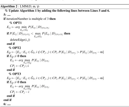
with the nodes to which they are assigned. Algorithm 2 details the changes to the forward selection of the simplified LMM (Algorithm 1: Lines 5-6).
Algorithm 2: LMM(D,ω,γ)
% Update Algorithm 1 by adding the following lines between Lines 5 and 6. 5: ....
ifiterationNumber is multiple of 3then % OPT1
Ei j←arg min Exy∈GˆS
P(Exy|D)[CPx,CPy]
ifP(Ei j|D)[CPi,CPj]< max Exy∈/GˆS
P(Exy|D)[CPx,CPy]then
deleteEdge(i,j) end if
% OPT2
EQ← {Ei j:Ei j∈GˆS,i∈/CPj, j∈CPi,P(Ei j|D)[CPj]>P(Ei j|D)[CPi]−ω} ifEQ6=/0then
Ei j←arg max Exy∈EQ
P(Exy|D)[CPy]
CPj←CPj∪i end if
% OPT3
EQ← {Ei j:Ei j∈GˆS,i∈CPj, j∈CPi,P(Ei j|D)[CPj]<P(Ei j|D)[CPi]−ω} ifEQ6=/0then
Ei j←arg min Exy∈EQ
P(Exy|D)[CPy]
CPj←CPj−i end if
end if 6: ....
Note, LMM algorithm is presented here in high level language. Details on how we implemented and optimized LMM are presented in the supplementary material and also can be seen in the source code which we are making available with this publication. In the case of applying OPT1-3, to avoid closed loops of adding and deleting the same edges or updating the same sets of neighbors, in our implementation, edges added in the last ten iterations are not considered for either of OPT1, OPT2, or OPT3 operations.
6.3.1 SIMULATEDEXAMPLE
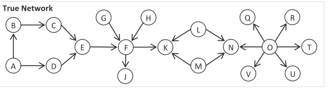
To illustrate the behavior of LMM, we simulated the network in Figure 1, and generated 1,000 samples as described in Section 7.1 below. We used a relatively large number of observations to ease the replication of our results and to test whether or how well LMM can recover the correct network given the proposed method of reducing independence testing when given a large set of samples.
O
V U
Q R
N T
L
M F
E
J
G H
K B
D A
C
True Network
Figure 1: A simulated network of 19 nodes and 20 edges
a result is expected, since once a node starts conditioning on child variables it can develop smaller partial correlations with its parent variables (see Supplement). On the other hand, nodeJ has only one parent and therefore, it will always be aware of it as a neighbor and hence its dependence on grandparent variables (nodesE,G, andH) or sibling variables (nodeK) will always be successfully blocked.
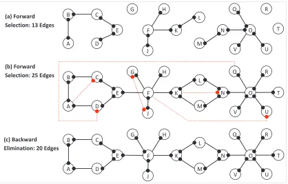
Figure 2 (b) shows a network of 25 edges recovered by continuing the forward selection for the same network and the same run of LMM. False edges are represented by red dotted lines. In this case, although the resulting connectivity information is not complete (distributed), it is sufficient to block candidate false edges. For example, all child variables of nodeOare aware ofOas a neighbor and therefore, their mutual dependence is blocked (e.g., P(EQR|D)[CPQ] ∼=0). On the other hand,
nodeOis only aware of three of its child variables and that does not have any effect of increasing the chances of recovering false edges among its child variables. Also, note that all the false edges recovered in Figure 2 (b) were only selected due to forcing LMM to recover more than 20 edges and the dependence along these edges is already blocked (e.g.,P(EJG|D)[CPJ]∼=0) and they will be
eliminated in the backward elimination phase as shown in Figure 2 (c).
The sub-network of nodeOand its child variables in Figure 2 is a good example of why LMM can outperform other algorithms such as the PC or MaxMin in limited sample problems. For exam-ple, in PC algorithm, to correctly recover the edgeEON, all independence tests of conditioning on all
subsets of the other 5 neighbors must be rejected while in LMM, nodeOwas aware of three neigh-bors only and therefore the chances of rejecting the edge due to multiple testing was reduced without increasing the risk of false positive edges among the child variables ofO. However, this is still a heuristic approach, and it is possible that in more complex examples the dependence along a false edge is only partially blocked (see the supplementary material for more examples and illustrations).
6.3.2 RANKING OFSKELETONEDGES
The LMM algorithm for skeleton recovery as given in Algorithm 1 can be used to recover skeletons in any of the following three approaches:
1. By using a threshold value (γ∈(0,1]) for the joint CPPD to decide which edges to be accepted or rejected.
2. By specifying the number of edges to be added in the forward selection and the number of edges to remain after backward elimination (MaxSize>MinSize>0, andγ=0).
O
V U
Q R
N T
L
M F
E
J
G H
K B D A C O
V U
Q R
N T
L
M F
E
J
G H
K B D A C O
V U
Q R
N T
L
M F
E
J
G H
K B D A C (a) Forward Selection: 13 Edges
(b) Forward Selection: 25 Edges
(c) Backward Elimination: 20 Edges
Figure 2: LMM output during forward selection and backward elimination of the same algorithm run at iterations where a) 13 edges have been added in forward selection, b) 25 edges have been added in forward selection, and c) 20 edges have remained in the skeleton after backward elimination has started. Red dotted lines represent false edges. A solid connection point (filled circle) at the end of an edge indicates the node is aware of its neighbor at the other side of the edge.
The order at which edges are deleted in the backward elimination is then used to rank edges where the last deleted edges become the most significant.
the edge with the least joint CPPD is deleted, and thus, the remaining edges are considered to have higher evidence of direct dependence (higher joint CPPD) and are thus more likely to be correct.
To our knowledge, this flexibility property of this last approach has no match in the algorithmic procedure of either the PC or the MaxMin algorithms where one needs to re-run the algorithm many times using different thresholds for independence testing to be able to rank edges. In addition, our approach can be used as a practical alternative to re-sampling and model averaging methods that are typically used to rank edges (Neapolitan, 2004). However, we should note that, ranking skeleton edges is not new to BN learning. For example, Tsamardinos and Brown (2008) ranked edges based on their p-values to control for false discovery rate in skeleton recovery. A similar approach for ranking edges was also proposed by Armen (2011).
In all experiments reported, the skeletons produced by LMM were generated using the proposed ranking procedure (Approach 3). The only exception of this configuration was the experiments of computational complexity comparison where we used a threshold parameter (Approach 1:γ∈(0,1]) for the joint CPPD in order to make the computational complexity comparison as fair as possible. Also, note that, one can also use a hybrid approach by using a non-zeroγin Approaches 2 and 3 above. This later case, however, is not used in any of the presented empirical results.
6.4 Complexity Analysis of Skeleton Recovery
The computational complexity of constraint-based methods is a measure of the number of inde-pendence tests needed to recover the skeleton. However, approximating the exact number of tests needed to execute LMM or other algorithms is a non-trivial problem. Alternatively and similar to other authors (Kalisch and B¨uhlmann, 2007; Tsamardinos et al., 2006), we use the worst case as an upper bound on the expected complexity.
In the worst case, the three algorithms, PC, MaxMin, and LMM, have a computational complex-ity ofO(p2×2q)wherepis the number of nodes andqis the maximum size of all neighbor sets in the recovered network (q=maxi|CPi|). This is because the worst case assumes all nodes have the
same maximum connectivity, and therefore we need to performO(p2×2q)independence tests to evaluate candidate edges. However, when using LMM with limited sample data, the proposed adap-tive reduction method of independence testing discussed in Section 6.2 (Algorithm 1: Lines 12-18) forces the algorithm to avoid using some neighbors in conditional independence tests. Therefore, although the node with the maximum connectivity is connected to qedges in the true DAG, dur-ing the skeleton recovery, it will only be aware of a fraction of them, leaddur-ing to a reduced number of independence tests (i.e.,O(p2×2q/δ)s.t.δ≥1). Unfortunately, estimating this fraction before running the algorithm is not possible. Therefore, in this paper, we mainly rely on the empirical evaluation to compare the time complexity of LMM to the other two algorithms.
One of the popular techniques to speed constraint-based learning is by limiting the size of the conditioning sets. This method can reduce computational complexity and it can be used with the PC, MaxMin or LMM algorithms. In the supplementary material, we elaborate on how we implemented LMM and on the optimization techniques we used to avoid redundant computations while making the search for the next edge to add or delete computationally efficient.
6.5 Extending the Skeleton to the Equivalence Class
of some Bayesian networks, in that, multiple networks with partially different orientations of edges can produce the same observational data. As a consequence, learning the complete directed graph from observational data alone can be impossible in many cases (Meek, 1995; Spirtes et al., 2001).
Once a skeleton is recovered, different approaches can be used to extend it to a CPDAG. Exam-ples of these methods are the score-based constrained hill climbing search algorithm (Tsamardinos et al., 2006) and the constraint-based approaches such as the PC algorithm (Meek, 1995; Spirtes et al., 2001). We stress that our contribution in recovering the skeleton can be used with any other algorithm to recover the CPDAG. However, in this work, we focus on constraint-based learning due to its easy implementation and its computational scalability. In addition, we improve upon the clas-sical constraint-based inference by presenting a new method for resolving conflicting v-structures.
Recovering CPDAGs using constraint-based inference relies on the recovery of the v-structures (see definitions) which are proven to be common among all DAGs of the same equivalence class. From properties of v-structure relations (see Lemma 13 below), a common child variable win a v-structure relation (x→w←y) induces a conditional dependence between the parent variablesx andy. Moreover, sincexandyare not adjacent in the skeleton,wcannot belong to any setZ\x,ythat
makesxandyconditionally independent. This property is the basic idea in constraint-based methods (Spirtes et al., 2001). However, this approach can produce inconsistent results. For example, in a case of limited training samples, it is possible to recover multiple conflicting v-structures.
To improve the accuracy of constraint-based inference of CPDAG, we present a new approach for ranking v-structures that can be used to resolve conflicts. The proposed method is derived from the following Lemma (see Neapolitan, 2004, Chapter 2):
Lemma 13 Suppose we have a DAG G= (V,E) and an uncoupled meeting x−w−y . Then the following are equivalent:
1. x−w−y is a head-to-head meeting: x→w←y.
2. There exists a set not containing w that d-separates x and y.
3. All sets containing w do not d-separate x and y.
Based on Lemma 13 and using the partial correlation method, when x→w←y is a correct v-structure and we have data with a large sample sizen, then both of the following statements are correct (see Appendix for proof):
1. lim
n→∞
min
Z⊆V\x,y,w
P(ρxy|Z6=0|ρˆxy|Z)
=0.
2. lim
n→∞
min
Z⊆V\x,y,w∈Z
P(ρxy|Z6=0|ρˆxy|Z)
=1.
Although, Lemma 13 was shown to be accurate in true DAGs (Neapolitan, 2004, Chapter 2), it might not always hold when learning DAGs in real applications due to the unguaranteed accuracy of independence testing methods based on small sample data. As a result, it is possible to recover wrong or conflicting results (e.g., conflicting v-structures:x→w←yandw→x←u).
the v-structure is a common child of the other two variables. To compute this confidence criterion for every candidate v-structure (x→w←y), we compute the joint CPPD (Equation 4) betweenx andy when w is added to all conditioning sets and the joint CPPD when wis removed from all the conditioning sets. The difference between the two joint CPPDs is then used as a measure of the level of the induced dependence betweenxandy caused byw. If the joint CPPD is found to increase whenwis added to all conditioning sets,wis concluded to be a common child of both x
andy. Also, in a case where two conflicting v-structures get accepted, we take advantage of the
amount of increase in the joint CPPD to perform tie-breaking and ignore the v-structure with the smaller induced dependence. The justification for this approach follows directly from Lemma 13, in that,winduces dependence betweenxandyif and only if it is their common child, and in small sample problems, it becomes intuitive to use the increase in the joint CPPD whenwis added to all conditioning sets as a measure of the confidence thatwis a common child.
Algorithm 3 presents a summary of the proposed constraint-based orientation of a given skele-ton. Note that, testing for induced dependence from common neighbors does not have the multiple testing problem. This is because the number of conditioning sets that contain the common neighbor is equal to the number of conditioning sets that do not contain the common neighbor. Therefore, in the orientation algorithm, we use the complete set of neighbors found in the skeleton. To distinguish these types of sets, we use bar notation on top of the set name (i.e.,CPx).
The set of additional orientation rules in Algorithm 3 are also used in other constraint based learning methods of the CPDAG such as the PC and TPDA algorithms. Meek (1995) provides a detailed discussion of these rules and their correctness for finding the CPDAG.
As mentioned earlier (Section 5.3), to our knowledge, there is only one other algorithm called Edge-Opt (Fast, 2010) that attempts to resolve conflicts in the constraint-based orientation of BN edges. Our approach is fundamentally different from Edge-Opt, in that, Edge-Opt considers all constraints to be equally significant, while our approach takes advantage of the differences in confi-dence at which the constraints are inferred and uses these differences to rank candidate v-structures. Moreover, in addition to being easy to implement, our approach does not require any heuristic search or computing a score criterion of the global network to perform tie-breaking. However, we should note that our approach does not solve conflicting edges resulting from the additional orientation rules (R1-4). In our implementation, whenever a conflict is found along a certain edge, it is left undirected.
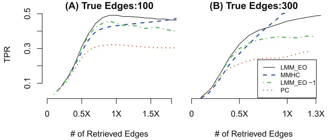
In the experimental validation, we were not able to empirically compare our approach to Edge-Opt because its publicly available implementation does not support the multivariate Gaussian case. Nonetheless, we compare our implementation to a variant of itself where a random tie-break is used to resolve conflicting v-structures and show that the proposed tie-breaking method provides a significant and consistent improvement in the accuracy of CPDAG orientation. We also compare the proposed approach to the PC and MaxMin hill climbing algorithms. Moreover, in the Appendix, we provide a complete proof that the proposed approach recovers the correct CPDAG in the asymptotic limit.
7. Experiments and Comparison
Algorithm 3: LMM EO(GS,D) Input: Skeleton:GS, Data:D
1: Q← /0 ///0is the empty set
2: for all hx,w,yiwhereExy∈/GSandEwy,Ewx∈GSdo
3: CDw+(x,w,y)← min Z⊆CPx,w∈Z
P(ρxy|Z6=0|ρˆxy|Z)× min
Z⊆CPy,w∈Z
P(ρxy|Z6=0|ρˆxy|Z)
4: CDw−(x,w,y)← min
Z⊆CPx,w∈/Z
P(ρxy|Z6=0|ρˆxy|Z)× min Z⊆CPy,w∈/Z
P(ρxy|Z6=0|ρˆxy|Z)
5: CD(x,w,y) =CDw+(x,w,y)−CDw−(x,w,y)
6: ifCD(x,w,y)>0then
7: Q←Q∪<x,w,y> 8: end if
9: end for
10: whileQis not emptydo
11: <x,w,y>← arg max
<j,k,l>∈QCD(j,k,l)
12: Q←Q−<x,w,y>
13: ifthe edgesx−wandy−ware not orientedthen
14: Orientx−wintox→w
15: Orienty−wintoy→w
16: end if
17: end while
% Apply the Additional Orientation Rules as Follows:
18: repeat
19: Orienti−jintoi→ jwhenever any of the following is correct:
20: R1: There exists an arrowk→i s.t.kand jare not adjacent.
21: R2: There exists a directed path fromito j(i.e.,i→ {} → j).
22: R3: There exist two chainsi−k→ jandi−l→ j.
23: R4: There exist two chainsi−k→landk→l→ j s.t.kandlare adjacent.
24: untilno more orientations are found
et al., 2010). The original MaxMin algorithm tool (Aliferis et al., 2003) only supports the discrete data case. We therefore re-implemented the algorithm to use the partial correlation test to recover the skeleton. For the CPDAG recovery, we used the publicly available toolkit BNlearn (Scutari, 2010) which implements a variant of MaxMin hill climbing that supports the BIC score criterion for continuous data, which we used for all MMHC reported experiments. Also, in all experiments, the hill climbing search was performed with a Tabu search with a list of 100 possible solutions which is the same setting used by the authors of the algorithm (Tsamardinos et al., 2006).
7.1 Simulating Data
For every experiment, the true model is randomly generated (Kalisch and B¨uhlmann, 2007) as follows:
2. Fill the adjacency matrixAwith zeros.
3. Randomly fill entries in the lower triangle matrix Awith ones by independent realizations of Bernoulli random variables with a success probabilityswhere 0<s<1 (srepresents the level of sparseness of the network)
4. Replace each entry with a 1 in the adjacency matrix by independent realizations of a uniform random variable in the range[−1,−0.1]∪[0.1,1].
These steps will result in an adjacency matrixAwhose entries are either zero or in the range [-1,-0.1] or [0.1,1]. Afterward, in the corresponding DAG, ifAi j is not zero, then node jis a parent
of nodeiwith a coefficient Ai j. Using this randomization setting, in the case of pvariables, the
expected number of neighborsCPi∗for a nodeican be estimated as: E(|CPi∗|) =s×(p−1), while the expected number of all edges can be estimated as: E(|G|) =s×(p−1)×p/2. Therefore, the density of the graph is linearly proportional tos. For the rest of this paper, when the simulated networks are said to containXedges, this meansswas selected so that the expected number of edges wasX. However, the exact number of edges in each network will vary slightly due to randomization. In our empirical analysis, we have generated a single set of observational samples from every simulated network. Once the adjacency matrix of the simulated network is fixed, every observational sample is recursively generated as follows:
X(1)=ε(1)∼N(0,σ21).
∀i=2,3...p:X(i)=ε(i)+ i−1
∑
j=1
Ai j×X(j),s.t.ε(i)∼N(0,σ2i).
whereε(1),ε(2), ....ε(p) are independent random normal variables representing the marginal noise.
In all reported experiments, the variances of these noise variables are randomly sampled from an inverse gamma distribution:σ2
i ∼InvGamma(α=2,β=1),∀i.
7.2 Results and Discussion
To evaluate the proposed algorithm we performed multiple experiments with various settings in an effort to cover a wide variety of possible cases. In every case, we simulated multiple networks and carried out a semi-exhaustive evaluation such that, all methods are compared at different levels of recovery where they are used to recover many solutions of varying sizes and the comparison is illustrated at each level. To finish all the results presented, we used 5 workstations with 8 cores each with a total computation time of about 4 weeks. Moreover, for computational reasons and due to the low statistical power when learning from limited sample data, the individual conditioning sets were restricted not to contain more than four variables for all methods. The only exception was the performance evaluation experiment based on large sample data where we let the conditioning sets contain up to six variables.
distance (SHD) metric. Every method was used to recover multiple skeletons or CPDAGs of vary-ing sizes for the same network and the evaluation plots (ROC, TPR, and SHD curves) of every method were then generated for every single network. For compact presentation, we only present the average of these evaluation curves for every set of networks in addition to bar plots of specified cases to demonstrate the variance of inference accuracy among all networks of the same set. In the case of PC and MaxMin, for every network, each algorithm was run many times with different thresholds (α=10−30, 10−10, 10−6, 10−4, 10−3, 0.003, 0.01, 0.02, 0.05, 0.1, 0.2, 0.3, 0.5). We also, in some cases, used additional alpha values greater than 0.5 to recover larger numbers of edges. In contrast, for all experiments except for computational complexity, LMM was run only once for every network using Approach 3 described in Section 6.3.2. In the forward selection, LMM was set to add as many edges as 2.5 times the number of nodes (MaxSize=2.5×numbero f nodes) and the order at which edges were removed in the backward elimination was used to rank all selected edges (MinSize=0). The choice of 2.5 was mainly to ensure that the number of edges added in the forward selection is large enough to work well for most cases.
7.2.1 SKELETONRECOVERY
In the first set of experiments, we evaluate LMM for recovering skeletons using 900 networks divided into 9 groups simulated as follows:
1. Fixed number of nodesp=200.
2. Three levels of connectivity density: ∼100,∼200, and∼400 edges.
3. Three levels of number of observations: 30, 100, and 300 samples.
4. For every configuration (same number of edges and same number of observations), a set of 100 different networks were generated with separate observational data for each.
First, to assess the effect of the new joint dependence criterion and the proposed adaptive re-duction of independence testing, we compared LMM to two variants of itself LMM-1 and LMM-2. In all experiments presented, LMM was configured to adaptively reduce the independence testing as described in Section 6.2 by settingωto very small value (ω=10−6). In contrast, LMM-1 and LMM-2 were configured not to use the adaptive reduction of independence testing by settingωto 1. Also, LMM-1 was set to use the proposed joint CPPD criterion (Equation 4) while LMM-2 was set to use the minimum of the one-sided CPPDs from both sides ( ˆP(Ei j |D)[CPi,CPj] =min(P(Ei j|
D)[CPi],P(Ei j |D)[CPj])) as a mutual dependence criterion which made it the most similar to the PC
and MaxMin algorithms in assessing edges.
Figure 3, shows an averaged plot of the false positive rate (FPR) and the true positive rate (TPR) of the three algorithms in recovering the skeletons of four sets of the simulated networks where the number of edges is∼100 and∼400 while the number of observations is 30 and 100 samples. In addition, Figure 4 shows the bar plots of the area under the ROC (auROC) for the three methods for skeleton recovery of 9 networks sets when the FPR is restricted to [0-0.06]. Note that, because these are partial ROC curves, the auROC is normalized by the maximum possible auROC which is 0.06.
(A) 30 Samples
FPR
T
PR
0.00 0.02 0.04 0.06
0 .3 0 0 .4 0 0 .5 0 0 .6 0
(B) 100 Samples
FPR
0.00 0.02 0.04 0.06
0 .5 5 0 .6 5 0 .7 5 100E_LMM 100E_LMM−1 100E_LMM−2 400E_LMM 400E_LMM−1 400E_LMM−2
Figure 3: Average ROC of skeleton recovery of LMM, LMM-1, and LMM-2 when the number of true edges is∼100, and∼400 and the number of observations is: A) 30 and B) 100 samples. X-Axis is the false positive rate (FPR) and Y-Axis is the average true positive rate (TPR).
LMM LMM −1 LMM −2
A) 30 Samples
a
u
R
O
C
100 200 400
0 .3 0 0 .4 0 0 .5 0
B) 100 Samples
# of True Edges
100 200 400
0 .5 5 0 .6 5 0 .7 5
C) 300 Samples
100 200 400
0 .7 5 0 .8 0 0 .8 5 0 .9 0
Figure 4: Bar plots of the auROC of skeleton recovery of LMM, LMM-1, and LMM-2 when the number of true edges is∼100,∼200, and ∼400 and the number of observations is: A) 30 B) 100 and C) 300 Samples. X-Axis is the correct number of edges in the true net-works and Y-Axis is the area under the partial ROC (auROC) where FPR is constrained to[0,0.06]. The plotted auROC is also normalized by the maximum possible area under the partial ROC.
to be a significant issue when recovering sparse networks where the variance of connection density is small. We also compared the performance of LMM to the PC and MaxMin algorithms. Figure 5 shows the average partial ROC of the three algorithms in recovering the skeletons of four network sets. Note that FPRs greater than 0.035 are ignored because solutions with more than 0.035 FPR are unlikely to have any practical use and it also is impractical to run the PC and MaxMin algorithms to recover denser skeletons since the number of required independence tests grows exponentially with the size of neighborhood.
In addition, we computed the area under the ROC curve where FPR is bounded to [0-0.035] for every case. Figure 6 shows the bar plots of the auROC for the three methods for the 9 network sets where the auROC is normalized by the maximum possible auROC, which is 0.035.
(A) 30 Samples
FPR
T
PR
0 0.01 0.02 0.03
0
.2
0
0
.3
0
0
.4
0
0
.5
0
(B) 100 Samples
FPR
0 0.01 0.02 0.03
0
.5
0
0
.6
0
0
.7
0
0
.8
0
100E_LMM 100E_PCAlg 100E_MaxMin 400E_LMM 400E_PCAlg 400E_MaxMin
Figure 5: Average ROC of skeleton recovery of LMM, PC, and MaxMin when the number of true edges is∼100, and∼400 and the number of observations is: A) 30 and B) 100 samples. X-Axis is the false positive rate (FPR) and Y-Axis is the average true positive rate (TPR).
Based on both Figures 5 and 6, LMM consistently outperforms both algorithms in all cases. Also, similar to first evaluation, the improvement is less significant when the correct graph is gen-erally sparse (i.e., 100 edges), since multiple testing is not an issue in very sparse graphs. The bar plots show the improvement to be consistent and not a result of outliers.
7.2.2 COMPUTATIONALCOMPLEXITY OFSKELETONRECOVERY
To experimentally compare the time complexity of the three algorithms (LMM, PC, and MaxMin) for skeleton recovery, we perform two types of comparisons. The first aims at evaluating the com-putational complexity when we have a large sample size, where the three algorithms can recover skeletons with high accuracy. The second comparison aims at evaluating the computational com-plexity when the sample size is limited.