International Journal of Engineering and Management Research, Vol.-2, Issue-6, December 2012
ISSN No.: 2250-0758
Pages: 40-47
www.ijemr.net
Analysis of Steady State Heat Conduction Problem Using EFGM
Manpreet Singh Brar1, Sunil Kumar2
1
M.Tech Student, 2Assistant Professor
Department of Mechanical Engineering, Yadvindra College of Engineering, Punjabi University Guru Kashi Campus Talwandi Sabo, Bathinda, Punjab, INDIA.
ABSTRACT
In present work, a one dimensional heat conduction problem with uniform heat generation is solved by using element free Gelerkin method (EFGM). The problem was to calculate the temperature distribution on different points across the thickness of a plane wall. The nodes are generated across the thickness of wall to find out the temperature distribution on different points. Then moving least squares (MLS) approximants is used to approximate the unknown function of temperature T(x) with the help of Th (x). Lagrange multiplier technique is used to enforce
essential boundary conditions. The MATLAB codes have been developed to obtain the solution of the given problem. The results obtained by EFG method are compared with analytical and FEM results to validate the proposed MATLAB codes. The results are also studied by increasing the number of nodes and by changing the values of scaling parameter dmax. Different weight functions
are also used to check the variation in the results.
Keywords: Element free Gelerkin method; Moving least squares approximants; Lagrange multiplier technique; One-dimensional heat conduction.
I. INTRODUCTION
In the present work a heat conduction problem is being solved by different methods such as analytical method, FEM and EFGM. EFGM was introduced by
Belytchko et al in 1994. Analytical and FE methods are being used from last so many years. The main objective of the work is to develop such a method which can replace these methods with more accuracy and less time consumption in computation. The biggest disadvantage of FEM is mesh generation, which becomes more difficult and time consuming for complicated problems. To overcome this difficulty lots of mesh free methods have been developed in last few decades
In mesh free methods nodes are used on problem domain and boundary to define the problem thus eliminating the burdensome work of mesh generation required in FEM. In meshless methods, interpolants are constructed solely on the basis of a set of scattered nodes
whereas in case of finite element method, interpoants are constructed by using a number of small elements known as finite elements. A number of meshless methods developed so far are:
Smoothed particle hydrodynamics (SPH) introduced
by Lucy, Gingold, and Monoghan in 1977. Diffuse
element method (DEM) was first introduced by Nayroles et al in 1992. Element Free Galerkin method introduced by
Belytchko et al in 1994. Moving Least Square
Reproducing Kernel Method (MLSRK) was proposed by
Liu et al [9] in 1995. Atluri and his co-workers introduced meshfree local Petrov-Galerkin formulation (MLPG). Another meshfree formulation formed by Atluri et al is the so-called local boundary integral equation (LBIE).
Singh [1] gave a three-dimensional numerical solution of composite heat transfer problems using mesh less element free Galerkin method (EFG). A comparison is made among the results obtained using proposed (exponential, rational and cosine) and existing (R&R, cubic spline, quartic spline, Gaussian, quadratic and hyperbolic) EFG weight functions with finite element method (FEM) for a three-dimensional composite heat transfer model problem. The validation of the EFG code has been achieved by comparing the EFG results with those obtained by FEM.
Liu et al [2] extended the rneshless weighted least squares (MWLS) method to solve conduction heat transfer problems. The MWLS formulation is first established for steady-state problems and then extended to unsteady-state problems with time-stepping schemes. Theoretical analysis and numerical examples indicate that larger time steps can be used in the present method than in meshless methods based on the Galerkin approach. Numerical studies show that the proposed method is a truly meshless method with good accuracy, high convergence rate, and high efficiency.
Belytschko et al. [3] developed Element Free
In this implementation, more accurate methods are used. One of the most startling discoveries in these studies is the high rates of convergence which were observed. Furthermore the method appears to be very effective for crack problems.
The goal of this work is to introduce the concepts involved in the implementation of EFGM to solve a steady state one dimensional heat conduction problem and show the effectiveness through several numerical applications. In Section 2 is devoted to discuss the methodology used in the present work and solution to the problems by analytical method, FEM and EFGM. Results are discussed in Section 3 with the help of tables and figures. And in Section 4 conclusion on the entire work is discussed along with future scope in Section 5.
II.
METHODOLOGY
In this work Element Free Galerkin method introduced by Belytchko et al[3] is used to solve a steady state one dimensional heat conduction problem. And for validation analytical method and FEM is used to find out the results for the same problem and these results are compared with EFGM results. The numerical chosen for this purpose is to find out temperature distribution across a large plate at various points considering that the heat conduction is one dimensional and under steady state. Two problems selected for validation and comparison are discussed as under:
Case study 1
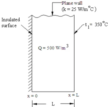
A plane wall is 1m thick and it has one surface (x = 0) insulated while the other surface (x = L) is maintained at a constant temperature of 350oC. The thermal conductivity of wall is 25 W/moC and a uniform heat generation per unit volume of 500 W/m3 exists throughout the wall. Determine the temperature distribution in the wall. [11]
Figure 1: Heat conduction through plane wall [11]
Analytical solution
First of all analytical method is used to find out the results. This method is time consuming, because in this
method the temperature distribution at different points across the wall is calculated one by one by using the following equation [11]
(1)
Where
= temperature maintained at surface (x = L) of
wall in oC.
L = thickness of plane wall in m.
Q = heat generated per unit volume in W/m3 k = thermal conductivity in W/moC
t = temperature on any point at distance x from surface (x = 0) of the wall in oC.
Case study 2
Heat is generated in a large plate (k = 0.8 W/moC) at the rate of 4000 W/m3. The plate is 25 cm thick. The outside surface of plate is exposed to ambient air at 30oC with a convective heat transfer coefficient of 20 W/m2 oC. Determine the temperature distribution in the wall. [12]
Figure 2: Heat conduction through plate with convection at outer face
Analytical solution
The result for this problem can also be found out by analytical method. In this method the temperature distribution across the plate can be found out by following equation. [11]
(2)
Where
= temperature of environment in oC. L = thickness of plane wall in m.
Q = heat generated per unit volume in W/m3 k = thermal conductivity in W/moC
FEM APPROACH
Both the above problems can be solved by using FEM. First of all a governing equation is selected for the given problem. In this case the governing equation is selected for a one dimensional steady state heat conduction problem, which is: [12]
(3)
After that element matrices are derived using Galerkin’s approach, which is given by: [12]
(4)
So element matrices (kT1;kT2; …..kTn) are generated
using the given values. These element matrices are assembled together to get global matrix K.
Similarly global matrix R, which is called heat rate vector, is assembled from element matrix rq given by:
(5)
And the stiffness equation is generated
K T = R (6)
Where matrix T gives the temperature distribution on the nodal points:
T = (7)
With the help of these formulas the results for temperature distribution on different points can be achieved.
EFGM APPROACH
Our attention is to solve a steady state heat conduction problem in one dimension. The main objective is to determine temperature distribution across a plane wall. In one dimensional steady state problem, the temperature gradient exists only along one axis, and temperature at any point does not depend upon time. So the governing equation for this type of problem can be given by using the general heat conduction equation in Cartesian coordinates as given below: [11]
The general heat conduction equation in Cartesian
coordinates is given as:
(8)
Consider heat conduction in a plane wall with uniform heat generation. Let Q (W/m3) is the internal heat
generated per unit volume. The thermal conductivity of the wall material is k. Heat conduction is taking place under steady state and in one dimension only.
Now as the heat conduction takes place under the
conditions, one dimensional and steady
state , then the above equation becomes:
(9)
Or
(10)
Now Gelerkin’s approach for the weak formulation is
(11)
Integrating above equation by parts
(12)
Rearranging equation, we get
(13)
[K]{T}= {f} (14)
Where the matrices [K] and {f} given by
(15)
(16) (17)
(18)
Enforcement of boundary conditions
Because the EFG shape function do not satisfy the Kronecker delta property, it creates some difficulty in the imposition of essential boundary conditions. Different numerical techniques are proposed by the researchers to enforce the boundary conditions such as:
4. Point collocation method 5. Coupling to finite elements
6. Use of specially modified shape functions etc. In this work Lagrange multiplier method is used to enforce the boundary conditions. In order to obtain the discrete equation from the weak form (Equation 13), the Lagrange multiplier λ is expressed by: [3]
λ(x) = NI(s) λI, x Γ
δλ(x) = NI(s)δλI, x Γ
After enforcing the boundary conditions using the Lagrangian multipliers the equation 14 can be written in the following form,
KT + G λ – f = 0 (19)
GTT – q = 0 (20)
OR
(21)
Moving least- squares approximation
The moving least square (MLS) approximation consists of three components: basis function, a weight function associated with each node, and asset of coefficients that depends on node position. The moving least squares interpolant Th(x) of function T(x) is defined in domain Ω by. [1][3][6]
Th(x) = = pT(x) a(x) (22) j=1,2,…,m Where p1(x) =1 and pj(x) are monomial basis in the
space coordinates xT=[x, y] so that the basis is complete. A linear and quadratic basis in one dimension can be given by
pT(x)=[1, x], m=2 (23a) pT(x)=[1, x, x2], m=3 (23b)
And linear and quadratic for two dimensions can be given as
pT(x)=[1, x, y], m=3 (24a)
pT(x)=[1, x, y, x2, xy, y2], m=6 (24b)
The unknown coefficients aj(x) are the functions of x;
a(x) is obtained at any point x by minimizing the weighted discrete L2-norm J:
(25)
Where n is the number of points in the neighborhood of x for which the weight function w(x-xi) ≠ 0 and Ti is the
nodal parameter at x= xi. And this neighborhood of x is
called domain of influence of x(or domain of influence of node i).
The relation between a(x) and T can be written in the linear equation which is:
A(x) a(x) =B(x) T (26)
Or
a(x) =A-1(x) B(x) T (27)
Where A and B are the matrices given by
(28)
(29)
Substituting a(x) in Eqn.(3.1), MLS approximant is given by
Th(x) = (30)
Where
(31)
TT = T1, T2, T3………, Tn (32)
The mesh free shape function is defined as
= (A-1(x) B(x))ji = p T
A-1 Bi
(33)
The continuity of the shape function i(x) is defined
by the continuity of basis function pj; depends on the
smoothness of the matrices A-1(x) and B(x) and choice of the weight function. The partial derivative of i(x) can be
calculated as
(34)
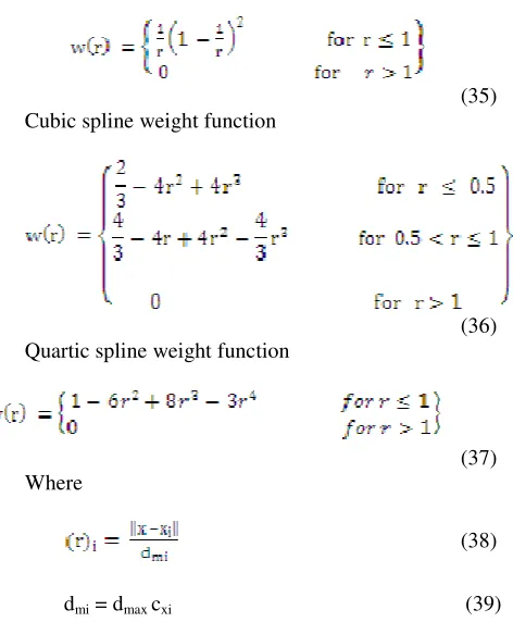
Weight functions
The weight function wt(x) = w(x - xi) plays an
important role in the performance of EFGM. It should be selected so that a unique solution a(x) can be generated. Its value should decrease in magnitude as the distance increases from x to xi. It is non zero over a small
neighborhood of node xi, called the support of node i. The
selected should be appropriate. The most commonly used weight functions are: [1]
Singular weight function
(35) Cubic spline weight function
(36) Quartic spline weight function
(37) Where
(38)
dmi = dmax cxi (39)
dmax is scaling parameter, cxi is the distance of i node
from nearest neighbors and the value of dmi is such that the
matrix is non-singular everywhere in the domain.
The cubic and quartic spline weight functions are more favorable because they provide continuity and less computationally less demanding. The singular weight function allows the direct imposition of essential boundary conditions. So in the case of singular weight function there is no need of Lagrange multipliers.
III.
RESULTS AND DISCUSSION
Case study 1
As mentioned in above section the results can be obtained by using analytical, FE and EFG methods. So the results obtained by these methods are discussed one by one below.
Analytical results
First of all analytical method is used to find out the results. If the length is divided in three equal parts then the analytical results are as shown in the table 1.
TABLE 1 ANALYTICAL RESULTS
NODES TEMPERATURE (in oC)
1 350
2 355.556
3 358.889
4 360
FEM results
With the help of the formulas given in section 3 the results for temperature distribution on different points are achieved which are shown in the table 2.
TABLE 2 FEM RESULT
NODES TEMPERATURE (in oC)
1 350
2 355.552
3 358.884
4 359.995
EFGM results
To find out results by EFGM a MATLAB code is generated by implementing MLS method, weak form and Lagrange multiplier technique. Temperature distribution across the wall can be achieved by putting the values of all the given parameters in the MATLAB program. The results thus obtained are shown in the table 3.
TABLE 3 EFGM RESULTS
NODES TEMPERATURE (in oC)
1 350.000
2 355.554
3 358.887
4 359.998
Validation for case study 1
Figure 3: Comparison between EFGM, Analytical, and FEM results
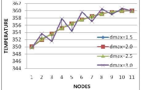
Effect of scaling parameter on the results
Figure 4 shows the EFGM results obtained by putting the different values of dmax. It can be seen clearly from
figure that the result obtained for dmax=1.5 is the best in
comparison to other three values. It can also be seen in the figure that as the value of dmax increases from 1.5 to 2 and
2.5 the percentage error in the result also increases. And if we further increase the value of dmax to 3 then the result
does not remain continues and consistent.
Figure 4: Effect of dmax on EFGM results
Case study 2
Similar to the first problem, the EFGM results are compared with analytical and FEM results as below. The problem is symmetric about the centerline of the plate. A two element finite element model is used to solve the problem. The left end is insulated (q = 0) because no heat can flow across a line of symmetry.
Analytical results
The result for this problem can also be found out by analytical method. In this method the temperature distribution across the plate can be found out by using equation 2.
TABLE 4 ANALYTICAL RESULTS
NODES TEMPERATURE (in oC)
1 55
2 84.3
3 94.07
FEM results
FEM method used in this problem is almost similar to the previous one and the results achieved for temperature distribution on different points are shown in the table 5 below.
TABLE 5 FEM RESULT
NODES TEMPERATURE (in oC)
1 55
2 84.3
3 94
EFGM results
To find out results by EFGM the MATLAB code similar to previous problem is used. In this case some of the input parameters are changed according to the requirement of the problem and thus temperature distribution across the wall is achieved by putting the values of all the given parameters in the MATLAB program. The results thus obtained are shown in the table 6 given below.
TABLE 6 EFGM RESULTS
NODES TEMPERATURE (in oC)
1 55.0000
2 84.2969
3 94.0625
Validation for case study 2
Figure 5: Comparison between EFGM, Analytical, and FEM results
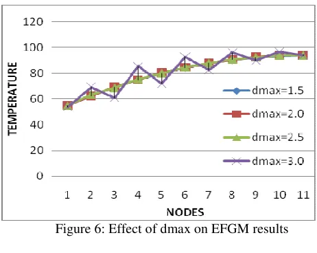
Effect of scaling parameter on the results
Figure 6 once again shows the EFGM results obtained by putting the different values of dmax. It can be seen
clearly again that the result obtained for dmax=1.5 is the
best in comparison to other three values. It can also be seen in this figure that as the value of dmax increases from
1.5 to 2 and 2.5 the percentage error in the result also increases. And if we further increase the value of dmax to 3
then the result does not remain continues and consistent. So from these results is clear that the best results can be achieved only by taking the value of scaling parameter dmax=1.5. Due to this reason all the EFGM results which
are compared with analytical and FEM results are obtained by taking dmax=1.5.
Figure 6: Effect of dmax on EFGM results
IV.
CONCLUSION
From the above steady it has been observed that EFG method is more accurate and less time consuming method than FEM. EFG method is an achievement in the improvement of mesh free methods. In this implementation EFG method is used and a MATLAB program has been developed to analyze one dimensional heat conduction problem with internal heat generation across a plane wall. The results obtained are compared with analytical and FEM results. It has been observed that the results obtained by EFGM are as accurate as analytical
or FEM results. The problem is solved by varying the number of nodes which gives the continuity of the results. Different weight functions are used to check the effect of the weight functions on temperature distribution. It is also concluded in this study that EFGM gives best results with dmax value ranging from 1 to 2. The biggest advantage of
EFGM is that there is no need of mesh generation due to which the time consumption for a given problem in comparison to FEM method is reduced. So, it is found that EFG method can be better alternate to analyze heat transfer and other problems.
VI. FUTURE SCOPE
In future this method can be extended to solve more complicated problems in 1D. This work can also be extended for more complex problems in 2D and 3D heat transfer. Lot of work has already been done in heat transfer problems by many researchers but still there is a scope for more study so that this method can be used to solve complicated engineering problems. This method can also be used to solve structural problems for stress strain analysis and for fluid flow analysis.
REFERENCES
[1]. I.V. Singh (2004). “A numerical solution of composite heat transfer problems using meshless method” International Journal of Heat and Mass Transfer, Vol. 47, pp 2123–2138.
[2]. Y. Liu, X. Zhang, M.W. Lu (2005). “A meshless method based on least-squares approach for steady- and unsteady-state heat conduction problems” Numerical Heat Transfer. Part B, 47, pp 257-275. [3]. T. Belytschko, Y.Y. Lu, L. Gu (1994). “Element-free
Galerkin methods”. International Journal of Numerical Methods in Engineering, vol. 37, pp 229-256.
[4]. Wing Kam Liu, Shaofan Li, Ted Belytschko (1996). “Moving Least Square Reproducing Kernel Methods (I) Methodology and Convergence” Computer Methods in Applied Mechanics and Engineering, Draft-Second(Revised)
[5]. J.H. Jeong, M.S. Jhon, J.S. Halow, J.V. Osdol (2003). “Smoothed particle hydrodynamics: Applications to heat conduction” Computer Physics Communications. Vol. 153, pp 71–84.
[6]. A. Singh, I.V. Singh, R. Prakash (2007). “Meshless element free Galerkin method for unsteady nonlinear heat transfer problems” International Journal of Heat and Mass Transfer, Vol. 50, pp 1212–1219.
Qinghai–Tibet railway embankment” Cold Regions Science and Technology, vol. 48, pp 15–23.
[8]. I.V. Singh, M. Tanaka, M. Endo (2008). “Element free Galerkin method for transient thermal analysis of carbon nanotube composites” Thermal science: Vol. 12, No. 2, pp. 39-48.
[9]. X.H. Zhang, J. Ouyang, L. Zhang (2009). “Matrix free meshless method for transient heat conduction problems” International Journal of Heat and Mass Transfer, Vol. 52, pp 2161–2165.
[10]. K. Sharma, V. Bhasin, I.V. Singh, B.K. Mishra (2010). “Effect of parameter in EFG (Element Free Galerkin) for 2-d analysis” International Journal of Engineering Science and Technology, Vol. 2(10), pp 5838-5844.
[11].R.K. Rajput (2003). “Heat and mass transfer” Edition 2nd.