Bayesian Network Structure Learning by Recursive Autonomy Identification

Bayesian Network Structure Learning by Recursive Autonomy

Identification

Raanan Yehezkel∗ [email protected]

Video Analytics Group NICE Systems Ltd.

8 Hapnina, POB 690, Raanana, 43107, Israel

Boaz Lerner [email protected]

Department of Industrial Engineering and Management Ben-Gurion University of the Negev

Beer-Sheva, 84105, Israel

Editor: Constantin Aliferis

Abstract

We propose the recursive autonomy identification (RAI) algorithm for constraint-based (CB) Bayes-ian network structure learning. The RAI algorithm learns the structure by sequential application of conditional independence (CI) tests, edge direction and structure decomposition into autonomous structures. The sequence of operations is performed recursively for each autonomous sub-structure while simultaneously increasing the order of the CI test. While other CB algorithms d-separate structures and then direct the resulted undirected graph, the RAI algorithm combines the two processes from the outset and along the procedure. By this means and due to structure decom-position, learning a structure using RAI requires a smaller number of CI tests of high orders. This reduces the complexity and run-time of the algorithm and increases the accuracy by diminishing the curse-of-dimensionality. When the RAI algorithm learned structures from databases representing synthetic problems, known networks and natural problems, it demonstrated superiority with respect to computational complexity, run-time, structural correctness and classification accuracy over the PC, Three Phase Dependency Analysis, Optimal Reinsertion, greedy search, Greedy Equivalence Search, Sparse Candidate, and Max-Min Hill-Climbing algorithms.

Keywords: Bayesian networks, constraint-based structure learning

1. Introduction

A Bayesian network (BN) is a graphical model that efficiently encodes the joint probability distri-bution for a set of variables (Heckerman, 1995; Pearl, 1988). The BN consists of a structure and a set of parameters. The structure is a directed acyclic graph (DAG) that is composed of nodes representing domain variables and edges connecting these nodes. An edge manifests dependence between the nodes connected by the edge, while the absence of an edge demonstrates independence between the nodes. The parameters of a BN are conditional probabilities (densities) that quantify the graph edges. Once the BN structure has been learned, the parameters are usually estimated (in the case of discrete variables) using the relative frequencies of all combinations of variable states as exemplified in the data. Learning the structure from data by considering all possible structures

haustively is not feasible in most domains, regardless of the size of the data (Chickering et al., 2004), since the number of possible structures grows exponentially with the number of nodes (Cooper and Herskovits, 1992). Hence, structure learning requires either sub-optimal heuristic search algorithms or algorithms that are optimal under certain assumptions.

One approach to structure learning—known as search-and-score (S&S) (Chickering, 2002; Cooper and Herskovits, 1992; Heckerman, 1995; Heckerman et al., 1995)—combines a strategy for searching through the space of possible structures with a scoring function measuring the fitness of each structure to the data. The structure achieving the highest score is then selected. Algorithms of this approach may also require node ordering, in which a parent node precedes a child node so as to narrow the search space (Cooper and Herskovits, 1992). In a second approach—known as constraint-based (CB) (Cheng et al., 1997; Pearl, 2000; Spirtes et al., 2000)—each structure edge is learned if meeting a constraint usually derived from comparing the value of a statistical or information-theory-based test of conditional independence (CI) to a threshold. Meeting such constraints enables the formation of an undirected graph, which is then further directed based on orientation rules (Pearl, 2000; Spirtes et al., 2000). That is, generally in the S&S approach we learn structures, whereas in the CB approach we learn edges composing a structure.

Search-and-score algorithms allow the incorporation of user knowledge through the use of prior probabilities over the structures and parameters (Heckerman et al., 1995). By considering several models altogether, the S&S approach may enhance inference and account better for model uncer-tainty (Heckerman et al., 1999). However, S&S algorithms are heuristic and usually have no proof of correctness (Cheng et al., 1997) (for a counter-example see Chickering, 2002, providing an S&S algorithm that identifies the optimal graph in the limit of a large sample and has a proof of correct-ness). As mentioned above, S&S algorithms may sometimes depend on node ordering (Cooper and Herskovits, 1992). Recently, it was shown that when applied to classification, a structure having a higher score does not necessarily provide a higher classification accuracy (Friedman et al., 1997; Grossman and Domingos, 2004; Kontkanen et al., 1999).

Algorithms of the CB approach are generally asymptotically correct (Cheng et al., 1997; Spirtes et al., 2000). They are relatively quick and have a well-defined stopping criterion (Dash and Druzdzel, 2003). However, they depend on the threshold selected for CI testing (Dash and Druzdzel, 1999) and may be unreliable in performing CI tests using large condition sets and a limited data size (Cooper and Herskovits, 1992; Heckerman et al., 1999; Spirtes et al., 2000). They can also be un-stable in the sense that a CI test error may lead to a sequence of errors resulting in an erroneous graph (Dash and Druzdzel, 1999; Heckerman et al., 1999; Spirtes et al., 2000). Additional infor-mation on the above two approaches, their advantages and disadvantages, may be found in Cheng et al. (1997), Cooper and Herskovits (1992), Dash and Druzdzel (1999), Dash and Druzdzel (2003), Heckerman (1995), Heckerman et al. (1995), Heckerman et al. (1999), Pearl (2000) and Spirtes et al. (2000). We note that Cowell (2001) showed that for complete data, a given node ordering and using cross-entropy methods for checking CI and maximizing logarithmic scores to evaluate structures, the two approaches are equivalent. In addition, hybrid algorithms have been suggested in which a CB algorithm is employed to create an initial ordering (Singh and Valtorta, 1995), to obtain a starting graph (Spirtes and Meek, 1995; Tsamardinos et al., 2006a) or to narrow the search space (Dash and Druzdzel, 1999) for an S&S algorithm.

undi-rected structure. This requires a number of CI tests growing exponentially with the number of nodes. This complexity is reduced in the PC algorithm to polynomial complexity by fixing the maximal number of parents a node can have and in the TPDA algorithm by measuring the strengths of the independences computed while CI testing along with making a strong assumption about the under-lying graph (Cheng et al., 1997). The TPDA algorithm does not take direct steps to restrict the size of the condition set employed in CI testing in order to mitigate the curse-of-dimensionality.

In the second stage, most CB algorithms direct edges by employing orientation rules in two con-secutive steps: finding and directing V-structures and directing additional edges inductively (Pearl, 2000). Edge direction (orientation) is unstable. This means that small errors in the input to the stage (i.e., CI testing) yield large errors in the output (Spirtes et al., 2000). Errors in CI testing are usually the result of large condition sets. These sets, selected based on previous CI test results, are more likely to be incorrect due to their size, and they also lead, for a small sample size, to poorer estimation of dependences due to the curse-of-dimensionality. Thus, we usually start learning using CI tests of low order (i.e., using small condition sets), which are the most reliable tests (Spirtes et al., 2000). We further note that the division of learning in CB algorithms into two consecutive stages is mainly for simplicity, since no directionality constraints have to be propagated during the first stage. However, errors in CI testing is a main reason for the instability of CB algorithms, which we set out to tackle in this research.

We propose the recursive autonomy identification (RAI) algorithm, which is a CB model that learns the structure of a BN by sequential application of CI tests, edge direction and structure de-composition into autonomous structures that comply with the Markov property (i.e., the sub-structure includes all its nodes’ parents). This sequence of operations is performed recursively for each autonomous sub-structure. In each recursive call of the algorithm, the order of the CI test is increased similarly to the PC algorithm (Spirtes et al., 2000). By performing CI tests of low order (i.e., tests employing small conditions sets) before those of high order, the RAI algorithm performs more reliable tests first, and thereby obviates the need to perform less reliable tests later. By directing edges while testing conditional independence, the RAI algorithm can consider parent-child relations so as to rule out nodes from condition sets and thereby to avoid unnecessary CI tests and to perform tests using smaller condition sets. CI tests using small condition sets are faster to implement and more accurate than those using large sets. By decomposing the graph into au-tonomous sub-structures, further elimination of both the number of CI tests and size of condition sets is obtained. Graph decomposition also aids in subsequent iterations to direct additional edges. By recursively repeating both mechanisms for autonomies decomposed from the graph, further re-duction of computational complexity, database queries and structural errors in subsequent iterations is achieved. Overall, the RAI algorithm learns faster a more precise structure.

Tested using synthetic databases, nineteen known networks, and nineteen UCI databases, RAI showed in this study superiority with respect to structural correctness, complexity, run-time and classification accuracy over PC, Three Phase Dependency Analysis, Optimal Reinsertion, a greedy hill-climbing search algorithm with a Tabu list, Greedy Equivalence Search, Sparse Candidate, naive Bayesian, and Max-Min Hill-Climbing algorithms.

2. Preliminaries

A BN B(

G

,Θ) is a model for representing the joint probability distribution for a set of variables X={X1. . .Xn}. The structure

G

(V,E)is a DAG composed of V, a set of nodes representing the domain variables X, and E, a set of directed edges connecting the nodes. A directed edge Xi→Xj connects a child node Xjto its parent node Xi. We denote Pa(X,

G

)as the set of parents of node X in a graph

G

. The set of parametersΘholds local conditional probabilities over X, P(Xi|Pa(Xi,

G

))∀i that quantify the graph edges. The joint probability distribution for X represented by a BN that is assumed to encode this distribution1is (Cooper and Herskovits, 1992; Heckerman, 1995; Pearl, 1988)

P(X1. . .Xn) = n

∏

i=1

P(Xi|Pa(Xi,

G

)). (1)

Though there is no theoretical restriction on the functional form of the conditional probability dis-tributions in Equation 1, we restrict ourselves in this study to discrete variables. This implies joint distributions which are unrestricted discrete distributions and conditional probability distributions which are independent multinomials for each variable and each parent configuration (Chickering, 2002).

We also make use of the term partially directed graph, that is, a graph that may have both directed and undirected edges and has at most one edge between any pair of nodes (Meek, 1995). We use this term while learning a graph starting from a complete undirected graph and removing and directing edges until uncovering a graph representing a family of Markov equivalent structures (pattern) of the true underlying BN2(Pearl, 2000; Spirtes et al., 2000). Pap(X,

G

), Adj(X,

G

)and

Ch(X,

G

)are, respectively, the sets of potential parents, adjacent nodes3and children of node X in a partially directed graph

G

, Pap(X,

G

) =Adj(X,

G

)\Ch(X,

G

).

We indicate that X and Y are independent conditioned on a set of nodes S (i.e., the condition set) using X ⊥⊥Y|S, and make use of the notion of d-separation (Pearl, 1988). Thereafter, we define d-separation resolution with the aim to evaluate d-separation for different sizes of condition sets, d-separation resolution of a graph, an exogenous cause to a graph and an autonomous sub-structure. We concentrate in this section only on terms and definitions that are directly relevant to the RAI concept and algorithm, where other more general terms and definitions relevant to BNs can be found in Heckerman (1995), Pearl (1988), Pearl (2000), and Spirtes et al. (2000).

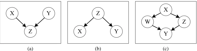
Definition 1 – d-separation resolution: The resolution of a d-separation relation between a pair of non-adjacent nodes in a graph is the size of the smallest condition set that d-separates the two nodes.

Examples of d-separation resolutions of 0, 1 and 2 between nodes X and Y are given in Figure 1.

Definition 2 – d-separation resolution of a graph: The d-separation resolution of a graph is the highest d-separation resolution in the graph.

The d-separation relations encoded by the example graph in Figure 2a and relevant to the de-termination of the d-separation resolution of this graph are: 1) X1⊥⊥X2|/0; 2) X1⊥⊥X4| {X3}; 3)

X1⊥⊥X5| {X3}; 4) X1 ⊥⊥X6| {X3}; 5) X2⊥⊥X4| {X3}; 6) X2⊥⊥X5| {X3}; 7) X2⊥⊥X6| {X3}; 8)

X3⊥⊥X6| {X4,X5}and 9) X4⊥⊥X5| {X3}. Due to relation 8, exemplifying d-separation resolution

1. Throughout the paper, we assume faithfulness of the probability distribution to a DAG (Spirtes et al., 2000). 2. Two BNs are Markov equivalent if and only if they have the same sets of adjacencies and V-structures (Verma and

Pearl, 1990).

X

Y

Z

X

Y

Z

X

Y

W

Z

(a) (b) (c)

Figure 1: Examples of d-separation resolutions of (a) 0, (b) 1 and (c) 2 between nodes X and Y .

of 2, the d-separation resolution of the graph is 2. Eliminating relation 8 by adding the edge X3→X6, we form a graph having a d-separation resolution of 1 (Figure 2b). By further adding edges to the graph, eliminating relations of resolution 1, we form a graph having a d-separation resolution of 0 (Figure 2c) that encodes only relation 1.

X X

X

X X

X

X X

X

X X

X

X X

X

X X

X

(a) (b) (c)

Figure 2: Examples of graph d-separation resolutions of (a) 2, (b) 1 and (c) 0.

Definition 3 – exogenous cause: A node Y in

G

(V,E)is an exogenous cause to

G

′(V′,E′), where V′⊂V and E′⊂E, if Y ∈/V′and∀X∈V′, Y ∈Pa(X,

G

)or Y∈/Adj(X,

G

)(Pearl, 2000).

Definition 4 – autonomous sub-structure: In a DAG

G

(V,E), a sub-structure

G

A(VA,EA) such that VA⊂V and EA⊂E is said to be autonomous in

G

given a set Vex⊂V of exogenous causes to

G

Aif∀X∈VA, Pa(X,

G

)⊂ {VA∪Vex}. If Vexis empty, we say the sub-structure is (completely) autonomous4.

We define sub-structure autonomy in the sense that the sub-structure holds the Markov property for its nodes. Given a structure

G

, any two non-adjacent nodes in an autonomous sub-structure

G

Ain

G

are d-separated given nodes either included in the sub-structure

G

Aor exogenous causes to

G

A. Figure 3 depicts a structure

G

containing a sub-structure

G

A. Since nodes X1 and X2 are exogenous causes to

G

A (i.e., they are either parents of nodes in

G

Aor not adjacent to them; see Definition 3),

G

Ais said to be autonomous in

G

given nodes X1and X2.

Proposition 1: If

G

A(VA,EA) is an autonomous sub-structure in a DAG

G

(V,E) given a set Vex⊂V of exogenous causes to

G

Aand X ⊥⊥Y|S, where X,Y ∈VA, S⊂V, then∃S′ such that S′⊂ {VA∪Vex}and X⊥⊥Y|S′.

X X

X

X

X

G

(

V

;

E

)

G

A

(

V

A

;

E

A

₎

Figure 3: An example of an autonomous sub-structure.

Proof: The proof is based on Lemma 1.

Lemma 1: If in a DAG, X and Y are non-adjacent and X is not a descendant of Y ,5 _{then X and Y} are d-separated given Pa(Y)(Pearl, 1988; Spirtes et al., 2000).

If in a DAG

G

(V,E), X⊥⊥Y|S for some set S, where X and Y are non-adjacent, and if X is not a descendant of Y , then, according to Lemma 1, X and Y are d-separated given Pa(Y). Since X and Y are contained in the sub-structure

G

A(VA,EA), which is autonomous given the set of nodes Vex, then, following the definition of an autonomous sub-structure, all parents of the nodes in VA— and specifically Pa(Y)—are members in set{VA∪Vex}. Then,∃S′ such that S′⊂ {VA∪Vex}and

X⊥⊥Y|S′, which proves Proposition 1.

3. Recursive Autonomy Identification

Starting from a complete undirected graph and proceeding from low to high graph d-separation res-olution, the RAI algorithm uncovers the correct pattern6of a structure by performing the following sequence of operations: (1) test of CI between nodes, followed by the removal of edges related to independences, (2) edge direction according to orientation rules, and (3) graph decomposition into autonomous sub-structures. For each autonomous sub-structure, the RAI algorithm is applied recursively, while increasing the order of CI testing.

CI testing of order n between nodes X and Y is performed by thresholding the value of a criterion that measures the dependence between the nodes conditioned on a set of n nodes (i.e., the condition set) from the parents of X or Y . The set is determined by the Markov property (Pearl, 2000), for example, if X is directed into Y , then only Y ’s parents are included in the set. Commonly, this criterion is theχ2goodness of fit test (Spirtes et al., 2000) or conditional mutual information (CMI) (Cheng et al., 1997).

5. If X is a descendant of Y , we change the roles of X and Y and replace Pa(Y)with Pa(X).

Directing edges is conducted according to orientation rules (Pearl, 2000; Spirtes et al., 2000). Given an undirected graph and a set of independences, both being the result of CI testing, the following two steps are performed consecutively. First, intransitive triplets of nodes (V-structures) are identified, and the corresponding edges are directed. An intransitive triplet X→Z←Y is defined

if 1) X and Y are non-adjacent neighbors of Z, and 2) Z is not in the condition set that separated X and Y . In the second step, also known as the inductive stage, edges are continually directed until no more edges can be directed, while assuring that no new V-structures and no directed cycles are created.

Decomposition into separated, smaller, autonomous sub-structures reveals the structure hierar-chy. Decomposition also decreases the number and length of paths between nodes that are CI-tested, thereby diminishing, respectively, the number of CI tests and the sizes of condition sets used in these tests. Both reduce computational complexity. Moreover, due to decomposition, additional edges can be directed, which reduces the complexity of CI testing of the subsequent iterations. Following de-composition, the RAI algorithm identifies ancestor and descendant sub-structures; the former are autonomous, and the latter are autonomous given nodes of the former.

3.1 The RAI Algorithm

Similarly to other algorithms of structure learning (Cheng et al., 1997; Cooper and Herskovits, 1992; Heckerman, 1995), the RAI algorithm7assumes that all the independences entailed from the given data can be encoded by a DAG. Similarly to other CB algorithms of structure learning (Cheng et al., 1997; Spirtes et al., 2000), the RAI algorithm assumes that the data sample size is large enough for reliable CI tests.

An iteration of the RAI algorithm starts with knowledge produced in the previous iteration and the current d-separation resolution, n. Previous knowledge includes

G

start, a structure having a d-separation resolution of n−1, and

G

_ex, a set of structures each having possible exogenous causes to

G

start. Another input is the graph

G

all, which contains

G

start,

G

exand edges connecting them. Note that

G

allmay also contain other nodes and edges, which may not be required for the learning task (e.g., edges directed from nodes in

G

startinto nodes that are not in

G

startor

G

_ex), and these will be ignored by the RAI. In the first iteration, n=0,

G

_ex= /0,

G

start(V,E) is the complete undirected graph and the d-separation resolution is not defined, since there are no pairs of d-separated nodes. Since

G

_exis empty,

G

all=

G

start.

Given a structure

G

starthaving d-separation resolution n−1, the RAI algorithm seeks indepen-dences between adjacent nodes conditioned on sets of size n and removes the edges corresponding to these independences. The resulting structure has a d-separation resolution of n. After applying orientation rules so as to direct the remaining edges, a partial topological order is obtained in which parent nodes precede their descendants. Childless nodes have the lowest topological order. This order is partial, since not all the edges can be directed; thus, edges that cannot be directed connect nodes of equal topological order. Using this partial topological ordering, the algorithm decomposes the structure into ancestor and descendent autonomous sub-structures so as to reduce the complexity of the successive stages.

First, descendant sub-structures are established containing the lowest topological order nodes. A descendant sub-structure may be composed of a single childless node or several adjacent childless

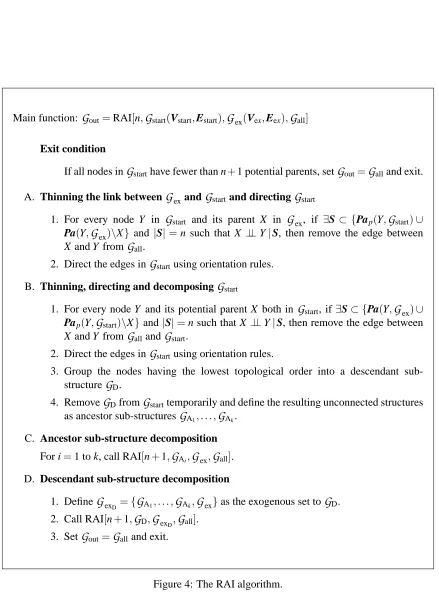
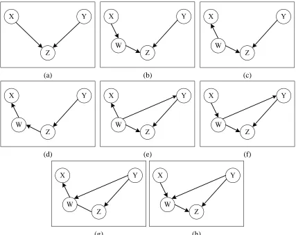
nodes. We will further refer to a single descendent sub-structure, although such a sub-structure may consist of several non-connected sub-structures. Second, all edges pointing towards nodes of the descendant sub-structure are temporarily removed (together with the descendant sub-structure itself), and the remaining clusters of connected nodes are identified as ancestor sub-structures. The descendent sub-structure is autonomous, given nodes of higher topological order composing the ancestor sub-structures. To consider smaller numbers of parents (and thereby smaller condition set sizes) when CI testing nodes of the descendant sub-structure, the algorithm first learns ancestor sub-structures, then the connections between ancestor and descendant sub-structures, and finally the descendant sub-structure itself. Each ancestor or descendent sub-structure is further learned by recursive calls to the algorithm. Figures 4, 5 and 6 show, respectively, the RAI algorithm, a manifesting example and the algorithm execution order for this example.

The RAI algorithm is composed of four stages (denoted in Figure 4 as Stages A, B, C and D) and an exit condition checked before the execution of any of the stages. The purpose of the exit condition is to assure that a CI test of a required order can indeed be performed, that is, the number of potential parents required to perform the test is adequate. The purpose of Stage A1 is to thin the link between

G

_ex and

G

start, the latter having d-separation resolution of n−1. This is achieved by removing edges corresponding to independences between nodes in

G

_ex and nodes in

G

startconditioned on sets of size n of nodes that are either exogenous to, or within,

G

start. Similarly, in Stage B1, the algorithm tests for CI of order n between nodes in

G

startgiven sets of size n of nodes that are either exogenous to, or within,

G

start, and removes edges corresponding to independences. The edges removed in Stages A1 and B1 could not have been removed in previous applications of these stages using condition sets of lower orders. When testing independence between X and Y , conditioned on the potential parents of node X , those nodes in the condition set that are exogenous to

G

startare X ’s parents whereas those nodes that are in

G

startare either its parents or adjacents.

In Stages A2 and B2, the algorithm directs every edge from the remaining edges that can be directed. In Stage B3, the algorithm groups in a descendant sub-structure all the nodes having the lowest topological order in the derived partially directed structure, and following the temporary re-moval of these nodes, it defines in Stage B4 separate ancestor sub-structures. Due to the topological order, every edge from a node X in an ancestor structure to a node Z in the descendant sub-structure is directed as X→Z. In addition, there is no edge connecting one ancestor sub-structure

to another ancestor sub-structure.

Thus, every ancestor sub-structure contains all the potential parents of its nodes, that is, it is au-tonomous (or if some potential parents are exogenous, then the sub-structure is auau-tonomous given the set of exogenous nodes). The descendant sub-structure is, by definition, autonomous given nodes of ancestor sub-structures. Proposition 1 showed that we can identify all the conditional in-dependences between nodes of an autonomous sub-structure. Hence, every ancestor and descendant sub-structure can be processed independently in Stages C and D, respectively, so as to identify con-ditional independences of increasing orders in each recursive call of the algorithm. Stage C is a recursive call for the RAI algorithm for learning each ancestor sub-structure with order n+1. Sim-ilarly, Stage D is a recursive call for the RAI algorithm for learning the descendant sub-structure with order n+1, while assuming that the ancestor sub-structures have been fully learned (having d-separation resolution of n+1).

Main function:

G

out=RAI[n,

G

start(Vstart,Estart),

G

_ex(Vex,Eex),

G

all]

Exit condition

If all nodes in

G

starthave fewer than n+1 potential parents, set

G

out=

G

alland exit. A. Thinning the link between

G

_exand

G

startand directing

G

start

1. For every node Y in

G

start and its parent X in

G

_ex, if ∃S ⊂ {Pap(Y,

G

start)∪ Pa(Y,

G

_ex)\X} and |S|=n such that X ⊥⊥Y|S, then remove the edge between X and Y from

G

all.

2. Direct the edges in

G

startusing orientation rules. B. Thinning, directing and decomposing

G

start

1. For every node Y and its potential parent X both in

G

start, if∃S⊂ {Pa(Y,

G

_ex)∪ Pap(Y,

G

start)\X}and|S|=n such that X ⊥⊥Y|S, then remove the edge between

X and Y from

G

alland

G

start.

2. Direct the edges in

G

startusing orientation rules.

3. Group the nodes having the lowest topological order into a descendant sub-structure

G

D.

4. Remove

G

Dfrom

G

starttemporarily and define the resulting unconnected structures as ancestor sub-structures

G

A1, . . . ,

G

Ak.

C. Ancestor sub-structure decomposition

For i=1 to k, call RAI[n+1,

G

Ai,

G

ex,

G

all]. D. Descendant sub-structure decomposition

1. Define

G

_ex

D ={

G

A1, . . . ,

G

Ak,

G

ex}as the exogenous set to

G

D. 2. Call RAI[n+1,

G

D,

G

exD,

G

all].

3. Set

G

out=

G

alland exit.

X1

X2

X3

X4 X5

X6

X7

X1

X2

X3

X6

X7

X4 X5

X1

X2

X3

X6

X7

X4 X5

(a) (b) (c)

X1

X2

X3

X6

X7

X4 X5

X1

X2

X3

X6

X7 G_A GA

G_D

X4 X5

X3

X4 X5

(d) (e) (f)

!"

! #

!$ !% !&

!'

!(

X1

X2

X3

X4 X5

X6

X7

(g) (h) (i)

)* +,-./ 0123 44 42567.16. / 899: ;<=>? @AB CDEFG @ CF @AHIIJ KLMNO PQR STU P T V P TWXY P SX

PQZ [[\

]^_`abc def gbf h b fijkbejb c l mmn op qrs tuv wxy t x z t x{|} t w uv wx~|} tuv wx  t x € t x |}| t u‚ ƒ ƒ„

RAI[2;G(fX…; X†g);fG(fX‡g);G(fXˆ; X ‰

; XŠg)g;G ‹ ŒŒ]

RAI[2;G(fXg);fG(fXŽ; Xg);G(fXg);G(fX ‘

; X’

; X“

g)g;G” •• ] 4 5 7 8 9 10 11 12 1 2 3 6

empty and

G

all=

G

start, so Stage A is skipped. In Stage B1, any pair of nodes in

G

startis CI tested given an empty condition set (i.e., checking marginal independence), which yields the removal of the edges between node X1and nodes X3, X4and X5 (Figure 5c). The edge directions inferred in Stage B2 are shown in Figure 5d. The nodes having the lowest topological order (X2, X6, X7) are grouped into a descendant sub-structure

G

D(Stage B3), while the remaining nodes form two unconnected ancestor sub-structures,

G

A1 and

G

A2 (Stage B4)(Figure 5e). Note that after decomposition, every

edge between a node, Xi, in an ancestor sub-structure, and a node, Xj, in a descendant sub-structure is a directed edge Xi→Xj. The set of all edges from an ancestor sub-structure to the descendant sub-structure is illustrated in Figure 5e by a wide arrow connecting the sub-structures. In Stage C, the algorithm is called recursively for each of the ancestor sub-structures with n=1,

G

start=

G

Ai (i=1,2) and

G

_ex= /0. Since sub-structure

G

A1 contains a single node, the exit condition for this

structure is satisfied. While calling

G

start=

G

A2, Stage A is skipped, and in Stage B1 the algorithm

identifies that X4⊥⊥X5|X3, thus removing the edge X4– X5. No orientations are identified (e.g., X3 cannot be a collider, since it separated X4 and X5), so the three nodes have equal topological order and they are grouped to form a descendant sub-structure. The recursive call for this sub-structure with n=2 is returned immediately, since the exit condition is satisfied (Figure 5f). Moving to Stage D, the RAI is called with n=1,

G

start=

G

D and

G

_ex={

G

A1,

G

A2}. Then, in Stage A1

relations X1⊥⊥ {X6,X7} |X2, X4⊥⊥ {X6,X7} |X2and{X3,X5} ⊥⊥ {X2,X6,X7} |X4are identified, and the corresponding edges are removed (Figure 5g). In Stage A2, X6 and X7 cannot collide at X2 (since X6 and X7are adjacent), and X2 and X6(X7) cannot collide at X7(X6) (since X2and X6 (X7) are adjacent); hence, no additional V-structures are formed. Based on the inductive step and since

X1is directed at X2, X2 should be directed at X6 and at X7. X6(X7) cannot be directed at X7 (X6), because no new V-structures are allowed (Figure 5h). Stage B1 of the algorithm identifies the relation X2⊥⊥X7|X6 and removes the edge X2→X7. In Stage B2, X6 cannot be a collider of X2 and X7, since it has separated them. In the inductive step, X6is directed at X7, X6→X7(Figure 5i). In Stages B3 and B4, X7and{X2,X6}are identified as a descendant sub-structure and an ancestor sub-structure, respectively. Further recursive calls (8 and 10 in Figure 6) are returned immediately, and the resulting partially directed structure (Figure 5i) represents a family of Markov equivalent structures (pattern) of the true structure (Figure 5a).

3.2 Minimality, Stability and Complexity

After describing the RAI algorithm (Section 3.1) and before proving its correctness (Section 3.3), we analyze in Section 3.2 three essential aspects of the algorithm—minimality, stability and complexity.

3.2.1 MINIMALITY

A structure recovered by the RAI algorithm in iteration m has a higher d-separation resolution and entails fewer dependences and thus is simpler and preferred8 to a structure recovered in iteration

m−k where 0<k≤m. By increasing the resolution, the RAI algorithm, similarly to the PC

algorithm, moves from a complete undirected graph having maximal dependence relations between variables to structures having less (or equal) dependences than previous structures, ending in a structure having no edges between conditionally independent nodes, that is, a minimal structure.

3.2.2 STABILITY

Similarly to Spirtes et al. (2000), we use the notion of stability informally to measure the number of errors in the output of a stage of the algorithm due to errors in the input to this stage. Similarly to the PC algorithm, the main sources of errors of the RAI algorithm are CI-testing and the identification of V-structures. Removal of an edge due to an erroneous CI test may lead to failure in correctly removing other edges, which are not in the true graph and also cause to orientation errors. Failure to remove an edge due to an erroneous CI test may prevent, or wrongly cause, orientation of edges. Missing or wrongly identifying a V-structure affect the orientation of other edges in the graph during the inductive stage and subsequent stages.

Many CI test errors (i.e., deciding that (in)dependence exists where it does not) in CB algo-rithms are the result of unnecessary large condition sets given a limited database size (Spirtes et al., 2000). Large condition sets are more likely to be inaccurate, since they are more likely to include unnecessary and erroneous nodes (erroneous due to errors in earlier stages of the algorithm). These sets may also cause poorer estimation of the criterion that measures dependence (e.g., CMI orχ2) due to the curse-of-dimensionality, as typically there are only too few instances representing some of the combinations of node states. Either way, these condition sets are responsible for many wrong decisions about whether dependence between two nodes exists or not. Consequently, these errors cause structural inaccuracies and hence also poor inference ability.

Although CI-testing in the PC algorithm is more stable than V-structure identification (Spirtes et al., 2000), it is difficult to say whether this is also the case in the RAI algorithm. Being recursive, the RAI algorithm might be more unstable. However, CI test errors are practically less likely to occur, since by alternating between CI testing and edge direction the algorithm uses knowledge about parent-child relations before CI testing of higher orders. This knowledge permits avoiding some of the tests and decreases the size of conditions sets of some other tests (see Lemma 1). In addition, graph decomposition promotes decisions about well-founded orders of node presentation for subsequent CI tests, contrary to the common arbitrary order of presentation (see, e.g., the PC algorithm). Both mechanisms enhance stability and provide some means of error correction, as will be demonstrated shortly.

Let us now extensively describe examples that support our claim regarding the enhanced sta-bility of the RAI algorithm. Suppose that following CI tests of some order both the PC and RAI algorithms identify a triplet of nodes in which two non-adjacent nodes, X and Y , are adjacent to a third node, Z, that is, X – Z – Y . In the immediate edge direction stage, the RAI algorithm identifies this triplet as a V-structure, X→Z←Y . Now, suppose that due to an unreliable CI test of a higher

order the PC algorithm removes X – Z and the RAI algorithm removes X →Z. Eventually, both

algorithms fail to identify the V-structure, but the RAI algorithm has an advantage over the PC algo-rithm in that the other arm of the V-structure is directed, Z←Y . This contributes to the possibility to

direct further edges during the inductive stage and subsequent recursive calls for the algorithm. The directed arm would also contribute to fewer CI tests and tests with smaller condition sets during CI testing with higher orders (e.g., if we later have to test independence between Y and another node, then we know that Z should not be included in the condition set, even though it is adjacent to Y ). In addition, the direction of this edge also contributes to enhanced inference capability.

Now, suppose another example in which after removing all edges due to reliable CI tests using condition set sizes lower than or equal to n, the algorithm identifies the V-structure X →Z ←Y

on a subsequent iteration using a larger condition set size (say n+1 without limiting the generality). We may be concerned that assuming a V-structure for the lower graph resolution, the RAI algorithm wrongly directs the second arm Z – Y as Z←Y . However, we demonstrate that the edge direction Z←Y remains valid even if there should be no edge X – Z in the true graph. Suppose that X →Z

was correctly removed conditioned on variable W , which is independent of Y given any condition set with a size smaller than or equal to n. Then, the possible underlying graphs are shown in Figures 7b-7d. The graph in Figure 7d is not possible, since it yields that X and Y are dependent given all condition sets of sizes smaller than or equal to n. In Figure 7b and Figure 7c, Z is a collider between

W and Y , and thus the edge direction Z←Y remains valid. A different graph, X→W←Z – Y (i.e.,

W is a collider), is not possible, since it means that X⊥⊥Z|S,|S| ≤n, W ∈/S and then X – Z should have been removed in a previous order (using condition set size of n or lower) and X →Z ←Y

should not have been identified in the first place. Now, suppose that W and Y are dependant. In this case, the possible graphs are those shown in Figures 7e-7h. Similarly to the case in which W and Y are independent, W cannot be a collider of X and Z (X→W←Z) in this case as well. The graphs

shown in Figures 7e-7g cannot be the underlying graphs since they entail dependency between

X and Y given a condition set of size lower than or equal to n. The graph shown in Figure 7h

exemplifies a V-structure X →W ←Y . Since we assume that X and Z are independent given W

(and thus X – Z was removed), a V-structure X →W ←Z is not allowed. Since the edge X→W

is already directed, the edge between W and Z must be directed as W →Z. In this case, to avoid

the cycle Y→W→Z→Y , the edge between Y and Z must be directed as in the true graph, that is, Y →Z.

Finally for the stability subsection, we note that the contribution of graph decomposition to structure learning using the RAI algorithm is threefold. First is the identification in early stages, using low-order, reliable CI tests, of the graph hierarchy, exemplifying the backbone of causal rela-tions in the graph. For example, Figure 5e shows that learning our example graph (Figure 5a) from the complete graph (Figure 5b) demonstrates, immediately after the first iteration, that the graph is composed of three sub-structures—{X1},{X2,X6,X7}and{X3,X4,X5}, where{X1} → {X2,X6,X7}

and{X3,X4,X5} → {X2,X6,X7}. This rough (low-resolution) partition of the graph is helpful in

visu-alizing the problem and representing the current knowledge from the outset and along the learning. The second contribution of graph decomposition is the possibility to implement learning using a parallel processor for each sub-structure independently. This advantage may be further extended in the recursive calls for the algorithm.

X Y

Z

X Y

Z W

X Y

Z W

(a) (b) (c)

X Y

Z W

X Y

Z W

X Y

Z W

(d) (e) (f)

X Y

Z W

X Y

Z W

(g) (h)

Figure 7: Graphs used to exemplify the stability of the RAI algorithm (see text).

accurate condition sets. Take, for example, CI testing for the redundant edge between X2 and X7 in our example graph (Figure 5i) if the RAI algorithm did not use decomposition. Graph decom-position for n=0 (Figure 5e) enables the identification of two ancestor sub-structures,

G

A1 and

G

A2, as well as a descendent sub-structure

G

D that are each learned recursively. During Stage D

(Figure 4) and while thinning the links between the ancestor sub-structures and

G

D (in Stage A1 of the recursion for n=1), we identify the relations X1⊥⊥ {X6,X7} |X2, X4 ⊥⊥ {X6,X7} |X2 and

{X3,X5} ⊥⊥ {X2,X6,X7} |X4and remove the 10 corresponding edges (Figure 5g). The decision to

test and remove these edges first was enabled by the decomposition of the graph to

G

A1,

G

A2 and

X2or X7). Instead, we perform in Stage B1 only one test, X2⊥⊥X7|X6. These benefits are the result of graph decomposition.

3.2.3 COMPLEXITY

CI tests are the major contributors to the (run-time) complexity of CB algorithms (Cheng and Greiner, 1999). In the worst case, the RAI algorithm will neither direct any edges nor decom-pose the structure and will thus identify the entire structure as a descendant sub-structure, calling Stages D and B1 iteratively while skipping all other stages. Then, the execution of the algorithm will be similar to that of the PC algorithm, and thus the complexity will be bounded by that of the PC algorithm. Given the maximal number of possible parents k and the number of nodes n, the number of CI tests is bounded by (Spirtes et al., 2000)

2

n

2

·

k

∑

i=0

n−1

i

≤n

2_(n−1)k−1

(k−1)! ,

which leads to complexity of O(nk).

This bound is loose even in the worst case (Spirtes et al., 2000) especially in real-world ap-plications requiring graphs having V-structures. This means that in most cases some edges are directed and the structure is decomposed; hence, the number of CI tests is much smaller than that of the worst case. For example, by decomposing our example graph (Figure 5) into descendent and ancestor sub-structures in the first application of Stage B4 (Figure 5e), we avoid checking

X6⊥⊥X7| {X1,X3,X4,X5}. This is because{X1,X3,X4,X5}are neither X6’s nor X7’s parents and thus are not included in the (autonomous) descendent sub-structure. By checking only X6⊥⊥X7| {X2}, the RAI algorithm saves CI tests that are performed by the PC algorithm. We will further elaborate on the RAI algorithm complexity in our forthcoming study.

3.3 Proof of Correctness

We prove the correctness of the RAI algorithm using Proposition 2. We show that only conditional independences (of all orders) entailed by the true underlying graph are identified by the RAI al-gorithm and that all V-structures are correctly identified. We then note on the correctness of edge direction.

Proposition 2: If the input data to the RAI algorithm are faithful to a DAG,

G

true, having any d-separation resolution, then the algorithm yields the correct pattern for

G

true.

Proof: We use mathematical induction to prove the proposition, where in each induction step, m, we prove that the RAI algorithm finds (a) all conditional independences of order m and lower, (b) no false conditional independences, (c) only correct V-structures and (d) all V-structures, that is, no V-structures are missing.

Base step (m=0): If the input data to the RAI algorithm was generated from a distribution faithful to a DAG,

G

true, having d-separation resolution 0, then the algorithm yields the correct pattern for

G

true.

there are no exogenous causes, Stage A is skipped. In Stage B, the algorithm tests for independence between every pair of nodes with an empty condition set, that is, X⊥⊥Y|/0(marginal independence), removes the redundant edges and directs the remaining edges as possible. In the resulting structure, all the edges between independent nodes have been removed and no false conditional independences are entailed. Thus, all the identified V-structures are correct, as discussed in Section 3.2.2 on stabil-ity, and there are no missing V-structures, since the RAI algorithm has tested independence for all pair of nodes (edges). At the end of Stage B2 (edge direction), the resulting structure and

G

truehave the same set of V-structures and the same set of edges. Thus, the correct pattern for

G

trueis identi-fied. Since the data entail only independences of zero order, further recursive calls with m≥1 will not find independences with condition sets of size m, and thus no edges will be removed, leaving the graph unchanged.

Inductive step (m+1): Suppose that at induction step m, the RAI algorithm discovers all condi-tional independences of order m and lower, no false condicondi-tional independences are entailed, all V-structures are correct, and no V-structures are missing. Then, if the input data to the RAI al-gorithm was generated from a distribution faithful to a DAG,

G

true, having d-separation resolution

m+1, then the RAI algorithm would yield the correct pattern for that graph.

In step m, the RAI algorithm discovers all conditional independences of order m and lower. Given input data faithful to a DAG,

G

true, having d-separation resolution m+1, there exists at least one pair of nodes, say{X,Y}, in the true graph, that has a d-separation resolution of m+1.9 Since the RAI, by the recursive call m+1 (i.e., calling RAI[m+1,

G

start,

G

_ex,

G

all]), has identified only conditional independences of order m and lower, an edge, EXY = (X – Y), exists in the input graph,

G

start. The smallest condition set required to identify the independence between X and Y is SXY (X ⊥⊥Y|SXY), such that|SXY| ≥m+1. Thus,|Pap(X)\Y| ≥m+1 or |Pap(Y)\X| ≥m+1, meaning that either node X or node Y has at least m+2 potential parents. Such an edge exists in at least one of the autonomous sub-structures decomposed from the graph yielded at the end of iteration m. When calling, in Stage C or Stage D, the algorithm recursively for this sub-structure with m′=m+1, the exit condition is not satisfied because either node X or node Y has at least m′+1 parents. Since Step m assured that the sub-structure is autonomous, it contains all the necessary node parents. Note that decomposition into ancestor,

G

A, and descendant,

G

D, sub-structures occurs after identification of all nodes having the lowest topological order, such that every edge from a node

X in

G

A to a node Y in

G

D is directed, X →Y . In the case that the sub-structure is an ancestor sub-structure, SXY contains nodes of the sub-structure and its exogenous causes. In the case that the sub-structure is a descendant sub-structure, SXY contains nodes from the ancestor sub-structures and the descendant sub-structure. Therefore, based on Proposition 1, the RAI algorithm tests all edges using condition sets of sizes m′and removes EXY (and all similar edges) in either Stage A or Stage B, yielding a structure with d-separation resolution of m′ and thereby yields the correct pattern for the true underlying graph of d-separation resolution m+1.

Spirtes (2001)—when introducing the anytime fast casual inference (AFCI) algorithm—proved the correctness of edge direction of AFCI. The AFCI algorithm can be interrupted at any stage (resolution), and the resultant graph at this stage is correct with probability one in the large sample

limit, although possibly less informative10 than if had been allowed to continue uninterrupted.11 Recall that interrupting learning means that we avoid CI tests of higher orders. This renders the resultant graph more reliable. We use this proof here for proving the correctness of edge direction in the RAI algorithm. Completing CI testing with a specific graph resolution n in the RAI algorithm and interrupting the AFCI at any stage of CI testing are analogous. Furthermore, Spirtes (2001) proves that interrupting the algorithm at any stage is also possible during edge direction, that is, once an edge is directed, the algorithm never changes that direction. In Section 3.2.2, we showed that even if a directed edge of a V-structure is removed, the direction of the remaining edge is still correct. Since directing edges by the AFCI algorithm after interruption yields a correct (although less informative) graph (Spirtes, 2001), also the direction of edges by the RAI algorithm yields a correct graph. Having (real) parents in a condition set used for CI testing, instead of potential parents, which are the result of edge direction for resolutions lower than n, is a virtue, as was confirmed in Section 3.1. All that is required that all parents, either real or potential, be included within the corresponding condition set, and this is indeed guaranteed by the autonomy of each sub-structure, as was proved above.

4. Experiments and Results

We compare the RAI algorithm with other state-of-the-art algorithms with respect to structural cor-rectness, computational complexity, run-time and classification accuracy when the learned structure is used in classification. The algorithms learned structures from databases representing synthetic problems, real decision support systems and natural classification problems. We present the experi-mental evaluation in four sections. In Section 4.1, the complexity of the RAI algorithm is measured by the number of CI tests required for learning synthetically generated structures in comparison to the complexity of the PC algorithm (Spirtes et al., 2000).

The order of presentation of nodes is not an input to the PC algorithm. Nevertheless, CI testing of orders higher than 0, and therefore also edge directing, which depends on CI testing, may be sensitive to that order. This may cause learning different graphs whenever the order is changed. Dash and Druzdzel (1999) turned this vice of the PC algorithm into a virtue by employing the partially directed graphs formed by using different orderings for the PC algorithm as the search space from which the structure having the highest value of the K2 metric (Cooper and Herskovits, 1992) is selected. For the RAI algorithm, sensitivity to the order of presentation of nodes is expected to be reduced compared to the PC algorithm, since the RAI algorithm, due to edge direction and graph decomposition, decides on the order of performing most of the CI tests and does not use an arbitrary order (Section 3.2.2). Nevertheless, to account for the possible sensitivity of the RAI and PC algorithms to this order, we preliminarily employed 100 different permutations12of the order for each of ten Alarm network (Beinlich et al., 1989) databases. Since the results of these experiments

10. Less informative in the sense that it answers “can’t tell” for a larger number of questions; that is, identifying, for example, “◦” edge endpoint (placing no restriction on the relation between the pair of nodes making the edge) instead of “→” endpoint.

11. The AFCI algorithm is also correct if hidden and selection variables exist. A selection variable models the possibility of an observable variable having some missing data. We focus here on the case where neither hidden nor selection variables exist.

had showed that the difference in performance for different permutations is slight, we further limited the experiments with the PC and RAI algorithms to a single permutation.

In Section 4.2, we present our methodology of selecting a threshold for RAI CI testing. We propose selecting a threshold for which the learned structure has a maximum of a likelihood-based score value.

In Section 4.3, we use the Alarm network (Beinlich et al., 1989), which is a widely accepted benchmark for structure learning, to evaluate the structural correctness of graphs learned by the RAI algorithm. The correctness of the structure recovered by RAI is compared to those of struc-tures learned using other algorithms—PC, TPDA (Cheng et al., 1997), GES (Chickering, 2002; Meek, 1997), SC (Friedman et al., 1999) and MMHC (Tsamardinos et al., 2006a). The PC and TPDA algorithms are the most popular CB algorithms (Cheng et al., 2002; Kennett et al., 2001; Marengoni et al., 1999; Spirtes et al., 2000); GES and SC are state-of-the-art S&S algorithms (Tsamardinos et al., 2006a); and MMHC is a hybrid algorithm that has recently been developed and showed superiority, with respect to different criteria, over all the (non-RAI) algorithms examined here (Tsamardinos et al., 2006a). In addition to correctness, the complexity of the RAI algorithm, as measured through the enumeration of CI tests and log operations, is compared to those of the other CB algorithms (PC and TPDA) for the Alarm network.

In Section 4.4, we extend the examination of RAI in structure learning to known networks other than the Alarm. Although the Alarm is a popular benchmark network, many algorithms perform well for this network. Hence, it is important to examine RAI performance on other networks for which the true graph is known. In the comparison of RAI to other algorithms, we included all the algorithms of Section 4.3, as well as the Optimal Reinsertion (OR) (Moore and Wong, 2003) algorithm and a greedy hill-climbing search algorithm with a Tabu list (GS) (Friedman et al., 1999). We compared algorithm performances with respect to structural correctness, run-time, number of statistical calls and the combination of correctness and run-time.

In Section 4.5, the complexity and run-time of the RAI algorithm are compared to those of the PC algorithm using nineteen natural databases. In addition, the classification accuracy of the RAI algorithm for these databases is compared to those of the PC, TPDA, GES, MMHC, SC and naive Bayesian classifier (NBC) algorithms. No structure learning is required for NBC and all the domain variables are used. This classifier is included in the study as a reference to a simple, yet accurate, classifier. Because we are interested in this section in classification, and a likelihood-based score does not reflect the importance of the class variable in structures used for classification (Friedman et al., 1997; Kontkanen et al., 1999; Grossman and Domingos, 2004; Yang and Chang, 2002), we prefer here the classification accuracy score in evaluating structure performance.

set of 5 and 10 for SC; and maximum number of parents allowed of 5, 10 and 20 and maximum allowed run time, which is one and two times the time used by MMHC on the corresponding data set, for OR. The only parameter that requires optimization in the RAI algorithm (similar to the other CB algorithms - PC and TPDA) is the CI testing threshold. We use no prior knowledge to find this threshold but a training set for each database (see Section 4.2 for details). Note, however that we do not account for the time required for selecting the threshold when reporting the execution time.

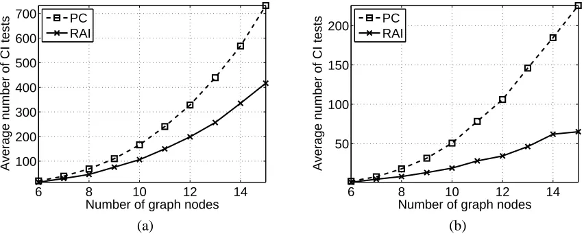
4.1 Experimentation with Synthetic Data

The complexity of the RAI algorithm was evaluated in comparison to that of the PC algorithm by the number of CI tests required to learn synthetically generated structures. Since the true graph is known for these structures, we could assume that all CI tests were correct and compare the numbers of CI tests required by the algorithms to learn the true independence relationships. In one experiment, all 29,281 possible structures having 5 nodes were learned using the PC and RAI algorithms. The average number of CI tests employed by each algorithm is shown in Figure 8a for increasing orders (condition set sizes). Figure 8b depicts the average percentages of CI tests saved by the RAI algorithm compared to the PC algorithm for increasing orders. These percentages were calculated for each graph independently and then averaged. It is seen that the advantage of the RAI algorithm over the PC algorithm is more prominent for high orders.

0 1 2 3

0 5 10 15 20 25

Condition set size

Average number of CI tests

PC RAI

0 1 2 3

0 10 20 30 40 50

Condition set size

CI tests reduction (%)

(a) (b)

Figure 8: Measured for increasing orders, the (a) average number of CI tests required by the RAI and PC algorithms for learning all possible structures having five nodes and (b) average over all structures of the reduction percentage in CI tests achieved by the RAI algorithm compared to the PC algorithm.

6 8 10 12 14 100

200 300 400 500 600 700

Number of graph nodes

Average number of CI tests

PC RAI

6 8 10 12 14

50 100 150 200

Number of graph nodes

Average number of CI tests

PC RAI

(a) (b)

Figure 9: Average number of CI tests required by the PC and RAI algorithms for increasing graph sizes and orders of (a) 3 and (b) 4.

computational time, is of order 3. Figure 9a shows the average numbers of CI tests performed for this order by the PC and RAI algorithms for graphs with increasing sizes. Moreover, because the maximal fan-in is 3, all CI tests of order 4 are a priori redundant, so we can further check how well each algorithm avoids these unnecessary tests. Figure 9b depicts the average numbers of CI tests performed by the two algorithms for order 4 and graphs with increasing sizes. Both Figure 9a and Figure 9b show that the number of CI tests employed by the RAI algorithm increases more slowly with the graph size compared to that of the PC algorithm and that this advantage is much more significant for the redundant (and more costly) CI tests of order 4.

We further expanded the examination of the algorithms in CI testing for different graph sizes and CI test orders. Figure 10 shows the average number and percentage of CI tests saved using the RAI algorithm compared to the PC algorithm for different condition set sizes and graph sizes. The number of CI tests having an empty condition set employed by each of the algorithms is equal and is therefore omitted from the comparison. The figure shows that the percentage of CI tests saved using the RAI algorithm increases with both graph and condition set sizes. For example, the saving in CI tests when using the RAI algorithm instead of the PC algorithm for learning a graph having 15 nodes and using condition sets of size 4 is above 70% (Figure 10b). In Section 4.4, we will demonstrate the RAI quality of requiring relatively fewer tests of high orders than of low orders for graphs of larger sizes for real, rather than synthetic, data.

4.2 Selecting the Threshold for RAI CI Testing

CI testing for the RAI algorithm can be based on theχ2test as for the PC algorithm or the conditional mutual information (CMI) as for the TPDA algorithm. The CMI between nodes X and Y conditioned on a set of nodes Z (i.e., the condition set), is:

CMI(X,Y|Z) =

NX

∑

i=1

NY

∑

j=1

NZ

∑

k=1

P(xi,yj,zk)·log

P(xi,yj|zk)

P(xi|zk)·P(yj|zk)

1 2 3 4 0

100 200 300 400

Condition set size

Average number of CI tests saved

6 9 12 15

1 2 3 4

0 20 40 60 80

Condition set size

CI tests saved (%)

6 9 12 15

(a) (b)

Figure 10: (a) Average number and (b) percentage of CI tests saved by using the RAI algorithm compared to the PC algorithm for graph sizes of 6, 9, 12 or 15 (gray shades) and orders between 1 and 4.

where xi and yj represent, respectively, states of X and Y , zk represents a combination of states of all variables in Z, and NX, NY and NZare the numbers of states of X , Y and Z, respectively.

In both CI testing methods, the value of interest (eitherχ2or CMI) is compared to a threshold. For example, CMI values that are higher or lower than the threshold indicate, respectively, condi-tional dependence or independence between X and Y given Z. However, the optimal threshold is unknown beforehand. Moreover, the optimal threshold is problem and data-driven, that is, it de-pends, on the one hand, on the database and its size and, on the other hand, on the variables and the numbers of their states. Thus, it is not possible to set a “default” threshold value that will accurately determine conditional (in)dependence while using any database or problem.

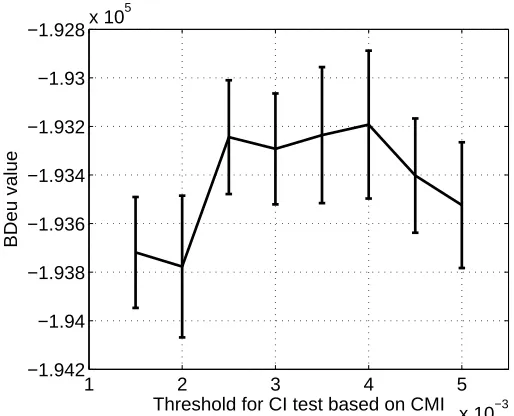
To find an optimal threshold for a database, we propose to score structures learned using differ-ent thresholds by a likelihood-based criterion evaluated using the training (actually validation) set and to select the threshold leading to the structure achieving the highest score. Such a score may be BDeu (Heckerman et al., 1995), although other scores (Heckerman et al., 1995) may also be ap-propriate. Note that BDeu scores equally statistically indistinguishable structures. Figure 11 shows BDeu values for structures learned by RAI for the Alarm network using different CMI threshold values. The maximum BDeu value was achieved at a threshold value of 4e-3 that was selected as the threshold for RAI CI testing for the Alarm network.

1 2 3 4 5 x 10−3 −1.942

−1.94 −1.938 −1.936 −1.934 −1.932 −1.93 −1.928x 10

5

Threshold for CI test based on CMI

BDeu value

Figure 11: BDeu values averaged over ten validation sets consisting of 10,000 samples each drawn from the Alarm network for increasing CMI thresholds used in CI testing for the RAI algorithm.

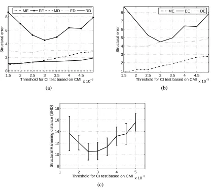
appears in the true graph but not in the learned graph. Finally, a reversed direction (RD) error is due to edge direction in the learned graph that is opposite to the edge direction in the true graph.

Figure 12a shows the sensitivity of the five structural errors to the CMI threshold. Each point on the graph is the average error over ten validation databases containing 10,000 randomly sampled instances each. Figure 12a demonstrates that the MD, RD and ED errors are relatively constant in the examined range of thresholds and the ME error increases monotonically. The EE error is the highest error among the five error types, and it has a minimum at a threshold value of 3e-3.

In Figure 12b, we cast the three directional errors using the total directional error (DE), DE = ED + MD + RD, and plot this error together with the ME and EE errors. The impact of each error for increasing thresholds is now clearer; the contribution of the DE error is almost constant, that of the ME error increases with the threshold but is less than DE, and that of the EE error dominants for every threshold.

1.5 2 2.5 3 3.5 4 4.5 x 10−3 0

2 4 6 8

Threshold for CI test based on CMI

Structural error

ME EE MD ED RD

1.5 2 2.5 3 3.5 4 4.5

x 10−3 1

2 3 4 5 6 7 8

Threshold for CI test based on CMI

Structural error

ME EE DE

(a) (b)

1 2 3 4 5

x 10−3 8

10 12 14 16 18

Structural Hamming distance (SHD)

Threshold for CI test based on CMI

(c)

Figure 12: Structural errors of the RAI algorithm learning the Alarm network for different CMI thresholds as averaged over ten validation sets of 10,000 samples each. (a) Five types (ME, EE, MD, ED and RD) of structural errors, (b) EE, ME and DE errors, and (c) SHD error (mean and std).

4.3 Learning the Alarm Network

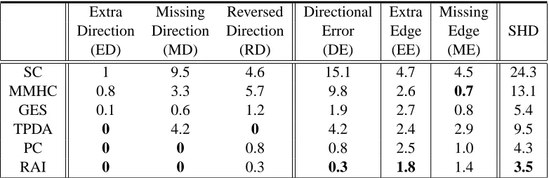
For evaluating the correctness of learned BN structures, we used the Alarm network, which is widely accepted as a benchmark for structure learning algorithms, since the true graph for this problem is known. The RAI algorithm was compared to the PC, TPDA, GES, SC and MMHC algorithms using ten databases containing 10,000 random instances each sampled from the network.

Extra Missing Reversed Directional Extra Missing

Direction Direction Direction Error Edge Edge SHD

(ED) (MD) (RD) (DE) (EE) (ME)

SC 1 9.5 4.6 15.1 4.7 4.5 24.3

MMHC 0.8 3.3 5.7 9.8 2.6 0.7 13.1

GES 0.1 0.6 1.2 1.9 2.7 0.8 5.4

TPDA 0 4.2 0 4.2 2.4 2.9 9.5

PC 0 0 0.8 0.8 2.5 1.0 4.3

RAI 0 0 0.3 0.3 1.8 1.4 3.5

Table 1: Structural errors of several algorithms as averaged over 10 databases each containing 10,000 randomly generated instances of the Alarm network. The total directional error is the sum of three different directional errors, DE=ED+MD+RD, and the SHD error is DE+EE+ME. Bold font emphasizes the smallest error over all algorithms for each type of structural error.

basis of the BDeu score hold. Moreover, usually such a score is used in both learning and evaluation of a structure; hence the score favors algorithms that use it in learning. Tsamardinos et al. (2006a) also mentioned that both scores do not rely on the true structure. Thus, they suggested the SHD metric, which is directly related to structural correctness, since it is the sum of the five errors of Section 4.2. Nevertheless, since SHD can be measured only when the true graph is known, scores such as BDeu and KL divergence are of great value in practical situations, for example, in classi-fication problems like those examined in Section 4.5 in which the true graph is not known. These scores are also beneficial in the determination of algorithm parameters. For example, in Section 4.2 we measured BDeu scores of structures learned using different thresholds in order to select a good threshold for RAI CI testing.

Although SHD sums all five structural errors, we were first interested in examining the contri-bution of each individual error to the total error. Table 1 summarizes the five structural errors for each algorithm as averaged over 10 databases of 10,000 instances each sampled from the Alarm network. These databases are different from those validation databases used for threshold setting. The table also shows the total directional error, DE, which is the sum of the three directional errors. Table 1 demonstrates that the lowest EE and DE errors are achieved by the RAI algorithm and the lowest ME error is accomplished by the MMHC algorithm. Computing SHD shows the advantage of the RAI (3.5) algorithm over the PC (4.3), TPDA (9.5), GES (5.4), MMHC (13.1) and the SC (24.3) algorithms. Further, we propose such a table as Table 1 as a useful tool for the identification of the sources of structural errors of a given structure learning algorithm.

Note that the SHD error weighs each of the five error types equally. We believe that a score that weighs the five types based on their relative significance to structure learning will be a more accurate method to evaluate structural correctness; however, deriving such a score is a topic for future research.

0 1 2 3 4 5 0 20 40 60 80 100

Condition set size

CI test reduction (%)

0% (0) 12% (160) 74% (422) 97% (243) 100% (64) 100% (4)

0 1 2 3 4 5 6

−100 −50 0 50 100

Condition set size

CI test reduction (%)

−112% (−587) 54% (170) 94% (112) 100% (28) 100% (1) 100% (6) 0% (0) (a) (b)

Figure 13: Average percentage (number) of CI tests reduced by using RAI compared to using (a) PC and (b) TPDA, as a function of the condition set size when learning the Alarm network.

percentage (and number) of CI tests reduced by using the RAI algorithm compared to using the PC or TPDA algorithms for increasing sizes of the condition sets. The RAI algorithm reduces the number of CI tests of orders 1 and above required by the PC algorithm and those of orders 2 and above required by the TPDA algorithm. Moreover, the RAI algorithm completely avoids the use of CI tests of orders 4 and above and almost completely avoids CI tests of order 3 compared to both the PC and TPDA algorithms. However, the RAI algorithm performs more CI tests of order 1 than the TPDA algorithm.

Figure 14 summarizes the total numbers of CI tests and log operations over different condition set sizes required by each algorithm. The RAI algorithm requires 46% less CI tests than the PC algorithm and 14% more CI tests (of order 1) than the TPDA algorithm. However, the RAI algorithm significantly reduces the number of log operations required by the other two algorithms. The PC or TPDA algorithms require, respectively, an additional 612% or 367% of the number of log operations required by the RAI algorithm. The reason for this substantial advantage of the RAI algorithm over both the PC and TPDA algorithms is the saving in CI tests of high orders (see Figure 13). These tests make use of large condition sets and thus are very expensive computationally.

4.4 Learning Known Networks