Learning From Crowds

Learning From Crowds

Vikas C. Raykar [email protected]

Shipeng Yu [email protected]

CAD and Knowledge Solutions (IKM CKS) Siemens Healthcare

Malvern, PA 19355 USA

Linda H. Zhao [email protected]

Department of Statistics University of Pennsylvania Philadelphia, PA 19104 USA

Gerardo Hermosillo Valadez [email protected]

Charles Florin [email protected]

Luca Bogoni [email protected]

CAD and Knowledge Solutions (IKM CKS) Siemens Healthcare

Malvern, PA 19355 USA

Linda Moy [email protected]

Department of Radiology

New York University School of Medicine New York, NY 10016 USA

Editor: David Blei

Abstract

For many supervised learning tasks it may be infeasible (or very expensive) to obtain objective and reliable labels. Instead, we can collect subjective (possibly noisy) labels from multiple experts or annotators. In practice, there is a substantial amount of disagreement among the annotators, and hence it is of great practical interest to address conventional supervised learning problems in this scenario. In this paper we describe a probabilistic approach for supervised learning when we have multiple annotators providing (possibly noisy) labels but no absolute gold standard. The proposed algorithm evaluates the different experts and also gives an estimate of the actual hidden labels. Experimental results indicate that the proposed method is superior to the commonly used majority voting baseline.

Keywords: multiple annotators, multiple experts, multiple teachers, crowdsourcing

1. Supervised Learning From Multiple Annotators/Experts

A typical supervised learning scenario consists of a training set

D

instances, wherexi∈

X

Y

corresponding known label. The task is to learn a function f :

X

Y

unseen data. Specifically for binary classification the supervision is from the set

Y

However, for many real life tasks, it may not be possible, or may be too expensive (or tedious)

to acquire the actual label yi for training—which we refer to as the gold standard or the

objec-tive ground truth. Instead, we may have multiple (possibly noisy) labels y1_i, . . . ,yR_i provided by R different experts or annotators. In practice, there is a substantial amount of disagreement among the experts, and hence it is of great practical interest to address conventional supervised learning algorithms in this scenario.

Our motivation for this work comes from the area of computer-aided diagnosis1(CAD), where

the task is to build a classifier to predict whether a suspicious region on a medical image (like a X-ray, CT scan, or MRI) is malignant (cancerous) or benign. In order to train such a classifier, a set of images is collected from hospitals. The actual gold standard (whether it is cancer or not) can only be obtained from a biopsy of the tissue. Since it is an expensive, invasive, and potentially dangerous process, often CAD systems are built from labels assigned by multiple radiologists who identify the locations of malignant lesions. Each radiologist visually examines the medical images and provides

a subjective (possibly noisy) version of the gold standard.2 The radiologist also annotates various

descriptors of the potentially malignant lesion, like the size (a regression problem), shape (a multi-class multi-classification problem), and also degree of malignancy (an ordinal regression problem). The radiologists come from a diverse pool including luminaries, experts, residents, and novices. Very often there is lot of disagreement among the annotations.

For a lot of tasks the labels provided by the annotators are inherently subjective and there will be substantial variation among different annotators. The domain of text classification offers such a scenario. In this context the task is to predict the category for a token of text. The labels for training are assigned by human annotators who read the text and attribute their subjective category.

With the advent of crowdsourcing (Howe, 2008) services like Amazon’s Mechanical Turk,3Games

with a Purpose,4and reCAPTCHA5it is quite inexpensive to acquire labels from a large number of

annotators (possibly thousands) in a short time (Sheng et al., 2008; Snow et al., 2008; Sorokin and

Forsyth, 2008). Websites such as Galaxy Zoo6allow the public to label astronomical images over

the internet. In situations like these, the performance of different annotators can vary widely (some may even be malicious), and without the actual gold standard, it may not be possible to evaluate the annotators.

In this work, we provide principled probabilistic solutions to the following questions:

1. How to adapt conventional supervised learning algorithms when we have multiple annotators providing subjective labels but no objective gold standard?

2. How to evaluate systems when we do not have absolute gold-standard?

3. A closely related problem—particularly relevant when there are a large number of annotators— is to estimate how reliable/trustworthy is each annotator.

1. See Fung et al. (2009) for an overview of the data mining issues in this area.

2. Sometimes even a biopsy cannot confirm whether it is cancer or not and hence all we can hope to get is subjective ground truth.

1.1 The Problem With Majority Voting

When we have multiple labels a commonly used strategy is to use the labels on which the majority of them agree (or average for regression problem) as an estimate of the actual gold standard. For

binary classification problems this amounts to using the majority label,7that is,

ˆ

yi= (

1 if (1/R)∑R_j=1y_ij>0.5 0 if (1/R)∑R

j=1y

j

i <0.5

,

as an estimate of the hidden true label and use this estimate to learn and evaluate classifiers/annotators. Another strategy is that of considering every pair (instance, label) provided by each expert as a sep-arate example. Note that this amounts to using a soft probabilistic estimate of the actual ground truth to learn the classifier, that is,

Pr[yi=1|yi1, . . . ,yRi] = (1/R) R

∑

j=1

y_ij.

Majority voting assumes all experts are equally good. However, for example, if there is only one true expert and the majority are novices, and if novices give the same incorrect label to a specific instance, then the majority voting method would favor the novices since they are in a majority. One could address this problem by introducing a weight capturing how good each expert is. But how would one measure the performance of an expert when there is no gold standard available?

1.2 Proposed Approach and Organization

To address the apparent chicken-and-egg problem, we present a maximum-likelihood estimator that jointly learns the classifier/regressor, the annotator accuracy, and the actual true label. For ease of exposition we start with binary classification problem in § 2. The performance of each annotator is measured in terms of the sensitivity and specificity with respect to the unknown gold standard (§ 2.1). The proposed algorithm automatically discovers the best experts and assigns a higher weight to them. In order to incorporate prior knowledge about each annotator, we impose a beta prior on the sensitivity and specificity and derive the maximum-a-posteriori estimate (§ 2.6). The final estimation is performed by an Expectation Maximization (EM) algorithm that iteratively establishes a particular gold standard, measures the performance of the experts given that gold standard, and refines the gold standard based on the performance measures. While the proposed approach is described using logistic regression as the base classifier (§ 2.2), it is quite general, and can be used with any black-box classifier (§ 2.7), and can also handle missing labels (that is, each expert is not required to label all the instances). Furthermore, we extend the proposed algorithm to handle categorical (§ 3), ordinal (§ 4), and regression problems (§ 5). In § 6 section we extensively validate our approach using both simulated data and real data from different domains.

1.3 Related Work and Novel Contributions

We first summarize the novel contributions of this work in context of other related work in this emerging new area. There has been a long line of work in the biostatistics and epidemiology litera-ture on latent variable models where the task is to get an estimate of the observer error rates based

on the results from multiple diagnostic tests without a gold standard (see Dawid and Skene, 1979, Hui and Walter, 1980, Hui and Zhou, 1998, Albert and Dodd, 2004 and references therein). In the machine learning community Smyth et al. (1995) first addressed the same problem in the context of labeling volcanoes in satellite images of Venus. We differ from this previous body of work in the following aspects:

1. Unlike Dawid and Skene (1979) and Smyth et al. (1995) which just focused on estimating the ground truth from multiple noisy labels, we specifically address the issue of learning a

classifier. Estimating the ground truth and the annotator/classifer performance is a byproduct

of our proposed algorithm.

2. In order to learn a classifier Smyth (1995) proposed to first estimate the ground truth (without using the features) and then use the probabilistic ground truth to learn a classifier. In contrast, our proposed algorithm learns the classifier and the ground truth jointly. Our experiments (§ 6.1.1) show that the classifier learnt and ground truth obtained by the proposed algorithm is superior to that obtained by other procedures which first estimates the ground truth and then learns the classifier.

3. Our solution is more general and can be easily extended to categorical(§ 3), ordinal(§ 4), and continuous data(§ 5). It can also be used in conjunction with any supervised learning algorithm. A preliminary version of this paper (Raykar et al., 2009) mainly discussed the binary classification problem.

4. Our proposed algorithm is also Bayesian—we impose a prior on the experts. The priors can potential capture the skill of different annotators. In this paper we refrain from doing a full Bayesian inference and use the mode of the posterior as a point estimate. A recent complete Bayesian generalization of these kind of models has been developed by Carpenter (2008).

5. The EM approach used in this paper is similar to that proposed by Jin and Ghahramani (2003). However their motivation is somewhat different. In their setting, each training example is annotated with a set of possible labels, only one of which is correct.

There has been recent interest in the natural language processing (Sheng et al., 2008; Snow et al., 2008) and computer vision (Sorokin and Forsyth, 2008) communities where they use Amazon’s Mechanical Turk to collect annotations from many people. They show that it can be potentially as good as that provided by an expert. Sheng et al. (2008) analyzed when it is worthwhile to acquire new labels for some of the training examples. There is also some theoretical work (see Lugosi, 1992 and Dekel and Shamir, 2009a) dealing with multiple experts. Recently Dekel and Shamir (2009b) presented an algorithm which does not resort to repeated labeling, that is, each example does not have to be labeled by multiple teachers. Donmez et al. (2009) address the issue of active learning in this scenario—How to jointly learn the accuracy of labeling sources and obtain the most informative labels for the active learning task? There has also been some work in the medical imaging community (Warfield et al., 2004; Cholleti et al., 2008).

2. Binary Classification

2.1 A Two-coin Model for Annotators

Let yj∈ {0,1}be the label assigned to the instancexby the jthannotator/expert. Let y be the actual

(unobserved) label for this instance. Each annotator provides a version of this hidden true label

based on two biased coins. If the true label is one, she flips a coin with biasαj (sensitivity). If the

true label is zero, she flips a coin with biasβj_{(specificity). In each case, if she gets heads she keeps}

the original label, otherwise she flips the label.

If the true label is one, the sensitivity (true positive rate) for the jthannotator is defined as the

probability that she labels it as one.

αj_:=Pr[yj_{=1|y=1]. (1)}

On the other hand, if the true label is zero, the specificity (1−false positive rate) is defined as the

probability that she labels it as zero.

βj_:=Pr[yj_{=0|y=0]. (2)}

The assumption introduced is thatαj andβj do not depend on the instancex. For example, in the

CAD domain, this means that the radiologist’s performance is consistent across different sub-groups of data.8

2.2 Classification Model

While the proposed method can be used for any classifier, for ease of exposition, we consider the

family of linear discriminating functions:

F

The final classifier can be written in the following form: ˆy=1 ifw⊤x≥γand 0 otherwise. The

thresholdγdetermines the operating point of the classifier. The Receiver Operating Characteristic

(ROC) curve is obtained as γ is swept from −∞ to ∞. The probability for the positive class is

modeled as a logistic sigmoid acting on fw, that is,

Pr[y=1|x,w] =σ(w⊤x),

where the logistic sigmoid function is defined asσ(z) =1/(1+e−z). This classification model is

known as logistic regression.

2.3 Estimation/Learning Problem

Given the training data

D

D

2.4 Maximum Likelihood Estimator

Assuming the training instances are independently sampled, the likelihood function of the

parame-tersθ={w,α,β}given the observations

D

Pr[D|θ] =

N

∏

i=1

Pr[y1

i, . . . ,yRi|xi,θ].

Conditioning on the true label yi, and also using the assumption yijis conditionally independent (of

everything else) givenαj,βjand yi, the likelihood can be decomposed as

Pr[D|θ] =

N

∏

i=1

Pr[y1_i, . . . ,yR_i|yi=1,α]Pr[yi=1|xi,w]

+ Pr[y1_i, . . . ,yR_i|yi=0,β]Pr[yi=0|xi,w] .

Given the true label yi, we assume that y1i, . . . ,yRi are independent, that is, the annotators make their

decisions independently.9 Hence,

Pr[y1

i, . . . ,yRi|yi=1,α] = R

∏

j=1

Pr[y_ij|yi=1,αj] = R

∏

j=1

[αj_]yij[₁−αj]1−y j i.

Similarly, we have

Pr[y1_i, . . . ,yR_i|yi=0,β] = R

∏

j=1

[βj]1−yij_[1−βj_]y j i_.

Hence the likelihood can be written as

Pr[D|θ] =

N

∏

i=1

aipi+bi(1−pi)

,

where we have defined

pi := σ(w⊤xi).

ai := R

∏

j=1

[αj_]yij[₁−αj]1−y j i.

bi := R

∏

j=1

[βj]1−yij[₁−βj]y j i.

The maximum-likelihood estimator is found by maximizing the log-likelihood, that is,

ˆ

θML={α,ˆ β,ˆ wˆ}=arg max

θ {ln Pr[D|θ]}.

2.5 The EM Algorithm

This maximization problem can be simplified a lot if we use the Expectation-Maximization (EM) algorithm (Dempster et al., 1977). The EM algorithm is an efficient iterative procedure to compute the maximum-likelihood solution in presence of missing/hidden data. We will use the unknown

hidden true label yi as the missing data. If we know the missing data y= [y1, . . . ,yN] then the

complete likelihood can be written as

ln Pr[D,y|θ] =

N

∑

i=1

yiln piai+ (1−yi)ln(1−pi)bi.

Each iteration of the EM algorithm consists of two steps: an Expectation(E)-step and a Maximization(M)-step. The M-step involves maximization of a lower bound on the log-likelihood that is refined in each iteration by the E-step.

1. E-step. Given the observation

D

conditional expectation (which is a lower bound on the true likelihood) is computed as

E{ln Pr[D,y|θ]}=

N

∑

i=1

µiln piai+ (1−µi)ln(1−pi)bi, (3)

where the expectation is with respect to Pr[y|

D

µi ∝ Pr[y1i, . . . ,yRi|yi=1,θ]·Pr[yi=1|xi,θ]

= aipi

aipi+bi(1−pi)

.

2. M-step. Based on the current estimate µiand the observations

D

then estimated by maximizing the conditional expectation. By equating the gradient of (3) to zero we obtain the following estimates for the sensitivity and specificity:

αj₌∑Ni=1µiyij ∑N

i=1µi

, βj=∑

N

i=1(1−µi)(1−yij)

∑N

i=1(1−µi)

.

Due to the non-linearity of the sigmoid, we do not have a closed form solution forwand we

have to use gradient ascent based optimization methods. We use the Newton-Raphson update

given bywt+1_=wt₋η_H−1_{g, wheregis the gradient vector,H is the Hessian matrix, and}

ηis the step length. The gradient vector is given by

g(w) =

N

∑

i=1

h

µi−σ(w⊤xi) i

xi.

The Hessian matrix is given by

H(w) =−

N

∑

i=1

h

σ(w⊤xi) i h

1−σ(w⊤xi) i

xix⊤i .

Essentially, we are estimating a logistic regression model with probabilistic labels µi.

These two steps (the E- and the M-step) can be iterated till convergence. The log-likelihood in-creases monotonically after every iteration, which in practice implies convergence to a local maxi-mum. The EM algorithm is only guaranteed to converge to a local maximaxi-mum. In practice multiple restarts with different initializations can potentially mitigate the local maximum problem. In this paper we use majority voting µi=1/R∑Rj=1y

j

2.6 A Bayesian Approach

In some applications we may want to trust a particular expert more than the others. One way to

achieve this is by imposing priors on the sensitivity and specificity of the experts. Sinceαj and

βj represent the probability of a binary event, a natural choice of prior is the beta prior. The beta

prior is also conjugate to the binomial distribution. For any a>0, b>0, andδ∈[0,1]the beta

distribution is given by

Beta(δ|a,b) =δ

a−1_(1−δ)b−1

B(a,b) ,

where B(a,b) =R1

0 δa−1(1−δ)b−1dδ is the beta function.We assume a beta prior10 for both the

sensitivity and the specificity as

Pr[αj|a₁j,a₂j] = Beta(αj|a₁j,a₂j). Pr[βj|b₁j,b₂j] = Beta(βj|b₁j,b₂j).

For sake of completeness we also assume a zero mean Gaussian prior on the weightswwith

in-verse covariance matrixΓ, that is, Pr[w] =

N

ˆ

θMAP=arg max

θ {ln Pr[D|θ] +ln Pr[θ]}.

An EM algorithm can be derived in a similar fashion for MAP estimation by relying on the inter-pretation of Neal and Hinton (1998). The final algorithm is summarized below:

1. Initialize µi= (1/R)∑Rj=1y

j

i based on majority voting.

2. Given µi, estimate the sensitivity and specificity of each annotator/expert as follows.

αj ₌ a j

1−1+∑Ni=1µiyij

a₁j+a₂j−2+∑N_i=1µi

.

βj ₌ b j

1−1+∑

N

i=1(1−µi)(1−yij)

b₁j+b₂j−2+∑N

i=1(1−µi)

. (4)

The Newton-Raphson update for optimizingwis given bywt+1=wt−ηH−1g, with step

lengthη, gradient vector

g(w) =

N

∑

i=1

h

µi−σ(w⊤xi) i

xi−Γw,

and Hessian matrix

H(w) =−

N

∑

i=1

σ(w⊤xi) h

1−σ(w⊤xi) i

xix⊤i −Γ.

10. It may be convenient to specify a prior in terms of the mean µ and variance σ2. The mean and the variance for a beta prior are given by µ=a/(a+b) and σ2 =ab/((a+b)2_{(a+b+1)). Solving for a and b we get}

3. Given the sensitivity and specificity of each annotator and the model parameters, update µias

µi=

aipi

aipi+bi(1−pi)

, (5)

where

pi = σ(w⊤xi).

ai = R

∏

j=1

[αj_]yij[₁−αj]1−y j i.

bi = R

∏

j=1

[βj]1−yij[₁−βj]y j

i. ₍₆₎

Iterate (2) and (3) till convergence.

2.7 Discussions

1. Estimate of the gold standard The value of the posterior probability µi is a soft

probabilis-tic estimate of the actual ground truth yi, that is, µi=Pr[yi=1|y1i, . . . ,yRi,xi,θ]. The actual

hidden label yi can be estimated by applying a threshold on µi, that is, yi=1 if µi≥γand

zero otherwise. We can useγ=0.5 as the threshold. By varyingγwe can change the

misclas-sification costs and obtain a ground truth with large sensitivity or large specificity. Because of this in our experimental validation we can actually draw an ROC curve for the estimated ground truth.

2. Log-odds ofµA particularly revealing insight can be obtained in terms of the log-odds or

the logit of the posterior probability µi. From (5) the logit of µi can be written as

logit(µi) =ln

µi 1−µi

=lnPr[yi=1|y

1

i, . . . ,yRi,xi,θ] Pr[yi=0|y1i, . . . ,yRi,xi,θ]

=w⊤xi+c+ R

∑

j=1

y_ij[logit(αj) +logit(βj)].

where c=∑R

j=1log1−α

j

βj is a constant term which does not depend on i. This indicates that

the estimated ground truth (in the logit form of the posterior probability) is a weighted linear

combination of the labels from all the experts. The weight of each expert is the sum of the

logit of the sensitivity and specificity.

3. Using any other classifier For ease of exposition we used logistic regression. However, the proposed algorithm can be used with any generalized linear model or in fact with any classifier that can be trained with soft probabilistic labels. In each step of the EM-algorithm,

the classifier is trained with instances sampled from µi. This modification is easy for most

probabilistic classifiers. For general black-box classifiers where we cannot tweak the training algorithm an alternate approach is to replicate the training examples according to the soft

label. For example a probabilistic label µi=0.8 can be effectively simulated by adding 8

4. Obtaining ground truth with no features In some scenarios we may not have featuresxi and we wish to obtain an estimate of the actual ground truth based only on the labels from multiple annotators. Here instead of learning a classifier we estimate p which is the prevalence

of the positive class, that is, p=Pr[yi=1]. We further assume a beta prior for the prevalence,

that is, Beta(p|p1,p2). The algorithm simplifies as follows.

(a) Initialize µi= (1/R)∑Rj=1y

j

i based on majority voting.

(b) Given µi, estimate the sensitivity and specificity of each annotator using (4). The

preva-lence of the positive class is estimated as follows.

p = p1−1+∑

N

i=1µi

p1+p2−2+N

.

(c) Given the sensitivity and specificity of each annotator and prevalence, refine µi as

fol-lows.

µi=

aip

aip+bi(1−p)

.

Iterate (2) and (3) till convergence. This algorithm is similar to the one proposed by Dawid and Skene (1979) and Smyth et al. (1995).

5. Handling missing labels The proposed approach can easily handle missing labels, that is,

when the labels from some experts are missing for some instances. Let Ri be the number of

radiologists labeling the ithinstance, and let Njbe the number of instances labeled by the jth

radiologist. Then in the EM algorithm, we just need to replace N by Nj for estimating the

sensitivity and specificity in (4), and replace R by Rifor updating µiin (6).

6. Evaluating a classifier We can use the probability scores µi directly to evaluate classifiers.

If zi are the labels obtained from any other classifier, then sensitivity and specificity can be

estimated as

α=∑

N

i=1µizi

∑N

i=1µi

, β=∑

N

i=1(1−µi)(1−zi)

∑N

i=1(1−µi)

.

7. Posterior approximation At the end of each EM iteration a crude approximation to the posterior is obtained as

αj ∼ Beta αj|a1j+

N

∑

i=1

µiyij,a j

2+

N

∑

i=1

µi(1−yij) !

,

βj ∼ Beta βj|b₁j+ N

∑

i=1

(1−µi)(1−yij),b j

2+

N

∑

i=1

(1−µi)yij !

.

3. Multi-class Classification

In this section we describe how the proposed approach for binary classification can be extended

to categorical data. Suppose there are K ≥2 categories. An example for categorical data from

different kinds on nodules. We can extend the previous model and introduce a vector of multinomial parametersαcj= (α_c1j , . . . ,α_cKj )for each annotator, where

αj

ck:=Pr[y

j_=k|y=c]

and∑K_k=1α_ckj =1. Hereα_ckj denotes the probability that the annotator j assigns class k to an instance

given the true class is c. When K=2, α₁₁j andα₀₀j are sensitivity and specificity, respectively. A

similar EM algorithm can be derived. In the E-step, we estimate

Pr[yi=c|

Y

∏

j=1

K

∏

k=1

(α_ckj )δ(yij,k),

whereδ(u,v) =1 if u=v and 0 otherwise and in the M-step we learn a multi-class classifier and

update the multinomial parameter as

αj

ck=

∑N

i=1Pr[yi=c|

Y

∑N

i=1Pr[yi=c|

Y

.

One can also assign a Dirichlet prior for the multinomial parameters, and this results in a smoothing term in the above updates in the MAP estimate.

4. Ordinal Regression

We now consider the situation where the outputs are categorical and have an ordering among the labels. In the CAD domain the radiologist often gives a score (for example, 1 to 5 from lowest to highest) to indicate how likely she thinks it is malignant. This is different from a multi-class setting in which we do not have any preference among the multiple class labels.

Let y_ij∈ {1, . . . ,K}be the label assigned to the ithinstance by the jth expert. Note that there is

an ordering in the labels 1< . . . <K. A simple approach is to convert the ordinal data into a series

of binary data (Frank and Hall, 2001). Specifically the K class ordinal labels are transformed into

K−1 binary class labels as follows:

y_ijc=

1 if y_ij>c

0 otherwise c=1, . . . ,K−1.

Applying the same procedure used for binary labels we can estimate Pr[yi>c]for c=1, . . . ,K−1.

The probability of the actual class values can then be obtained as

Pr[yi=c] =Pr[yi>c−1 and yi≤c] =Pr[yi>c−1]−Pr[yi>c].

The class with the maximum probability is assigned to the instance.

5. Regression

5.1 Model for Annotators

Let y_ij∈Rbe the continuous target value assigned to the ithinstance by the jthannotator. Our model

is that the annotator provides a noisy version of the actual true value yi. For the jth annotator we

will assume a Gaussian noise model with mean yi (the true unknown value) and inverse-variance

(precision)τj, that is,

Pr[y_ij|yi,τj] =

N

where the Gaussian distribution is defined as

N

unknown inverse-varianceτj measures the accuracy of each annotator—the larger the value of τj

the more accurate the annotator. We have assumed thatτjdoes not depend on the instancexi. For

example, in the CAD domain, this means that the radiologist’s accuracy does not depend on the nodule she is measuring. While this a practical assumption, it is not entirely true. It is known that some nodules are harder to measure than others.

5.2 Linear Regression Model for Features

As before we consider the family of linear regression functions:

F

, fw(x) =w⊤x. We assume that the actual target response y_iis given by the deterministic regression

function fwwith additive Gaussian noise, that is,

yi=w⊤xi+ε,

whereεis a zero-mean Gaussian random variable with inverse-variance (precision)γ. Hence

Pr[yi|xi,w,γ] =

N

5.3 Combined Model

Combining both the annotator (7) and the regressor (8) model we have

Pr[y_ij|xi,w,τj,γ] =

Z

Pr[y_ij|yi,τj]Pr[yi|xi,w,γ]dyi=

N

Since the two precision terms (γand τj) are grouped together they are not uniquely identifiable.

Hence we will define a new precision termλjas

1 λj =

1 γ+

1 τj.

So we have the following model

Pr[y_ij|xi,w,λj] =

N

5.4 Estimation/Learning Problem

Given the training data

D

D

{xi,y1i, . . . ,yRi}Ni=1, the task is to estimate the weight vectorwand the precisionλ= [λ1, . . . ,λR]of

5.5 Maximum-likelihood Estimator

Assuming the instances are independent the likelihood of the parameters θ={w,λ} given the

observations

D

Pr[D|θ] =

N

∏

i=1

Pr[y1_i, . . . ,yR_i|xi,θ].

Conditional on the instancexi we assume that y1i, . . . ,yRi are independent, that is, the annotators

provide their responses independently. Hence from (9) the likelihood can be written as

Pr[D|θ] =

N

∏

i=1

R

∏

j=1

N

The maximum-likelihood estimator is found by maximizing the log-likelihood

b

θML={bλ,wb}=arg max

θ {ln Pr[D|θ]}.

By equating the gradient of the log-likelihood to zero we obtain the following update equations for the precision and the weight vector.

1 b_λj =

1

N

N

∑

i=1

y_ij−w_b⊤xi

2 . (10) b w = N

∑

i=1

xix⊤i !−1 _N

∑

i=1

xi ∑R

j=1bλjy

j i ∑R

j=1bλj

!

. (11)

As the parametersw_bandλbare coupled together we iterate these two steps till convergence.

5.6 Discussions

1. Is this standard least-squares? Define the design matrix X = [x1, . . . ,xN]⊤ and the

re-sponse vector for each annotator asyj _{= [y}j

1, . . . ,y

j

N]⊤. Using matrix notation Equation 11

can be written as

b

w= (X⊤X)−1X⊤y_b where y_b=∑

R

j=1bλjyj

∑R

j=1bλj

. (12)

Equation 12 is essentially the solution to a standard linear regression model, except that we are

training a linear regression model withy_bas the ground truth, which is a precision weighted

mean of the response vectors from all the annotators. The variance of each annotator is

estimated using (10). The final algorithm iteratively establishes a particular gold standard (y_b),

measures the performance of the annotators and learns a regressor given that gold standard, and refines the gold standard based on the performance measures.

2. Are we better than the best annotator? If we assume λb is fixed (i.e., we ignore the

vari-ability and assume that it is well estimated) then ˆw is an unbiased estimator ofw and the

covariance matrix is given by

Cov(wˆ) =Cov(y_b)X⊤X−1= 1

∑R

j=1bλj

Since∑R_j=1bλj>maxj(bλj)the proposed method has a lower variance than the regressor learnt with the best annotator (i.e., the one with the minimum variance).

3. Are we better than the average? For a fixedXthe error inw_bdepends only on the variance

ofy_bj. If we know the trueλj then_byi is the best linear unbiased estimator for yi which

mini-mizes the variance. To see this consider any linear estimator of the formy_bi=∑jaj(y

j

i−bj).

The variance is given by Var[y_bi] =∑j(aj)2/λj. Since E[ybi] =yi∑jaj, for the bias of this

es-timator to be zero we require that∑jaj=1. Solving the constrained minimization problem

we see that aj=λj/∑jλjminimizes the variance.

4. Obtaining a consensus without features When no features are available the same algorithm can be simplified to get a consensus estimate of the actual ground truth and also evaluate the annotators. Essentially we have to iterate the following two updates till convergence

b

yi= ∑R

j=1bλjy

j i ∑R

j=1bλj

1 b_λj =

1

N

N

∑

i=1

y_ij−y_bi 2

.

6. Experimental Validation

We now experimentally validate the proposed algorithms on both simulated and real data.

6.1 Classification Experiments

We use two CAD and one text data set in our experiments. The CAD data sets include a digital mammography data set and a breast MRI data set, both of which are biopsy proven, that is, the gold standard is available. For the digital mammography data set we simulate the radiologists in order to validate our methods. The breast MRI data has annotations from four radiologists. We also report results on a Recognizing Textual Entailment data collected by Snow et al. (2008) using the Amazon’s Mechanical Turk which has annotations from 164 annotators.

6.1.1 DIGITALMAMMOGRAPHY WITHSIMULATEDRADIOLOGISTS

Mammograms are used as a screening tool to detect early breast cancer. CAD systems search for abnormal areas (lesions) in a digitized mammographic image. These lesions generally indicate the presence of malignant cancer. The CAD system then highlights these areas on the images, alerting the radiologist to the need for a further diagnostic mammogram or a biopsy. In classification terms, given a set of descriptive morphological features for a region on a image, the task is to predict whether it is potentially malignant (1) or not (0). In order to train such a classifier, a set of mammograms is collected from hospitals. The ground truth (whether it is cancer or not) is obtained from biopsy. Since biopsy is an expensive, tedious, and an invasive process, very often CAD systems are built from labels collected from multiple expert radiologists who visually examine the mammograms and mark the lesion locations—this constitutes our ground truth (multiple labels) for learning.

we can simultaneously (1) learn a logistic-regression classifier, (2) estimate the sensitivity and speci-ficity of each radiologist, and (3) estimate the golden ground truth. We compare the results with the classifier trained using the biopsy proved ground truth as well as the majority-voting baseline. For the first set of experiments we use 5 radiologists with sensitivity α= [0.90 0.80 0.57 0.60 0.55]

and specificityβ= [0.95 0.85 0.62 0.65 0.58]. This corresponds to a scenario where the first two radiologists are experts and the last three are novices. Figure 1 summarizes the results. We compare on three different aspects: (1) How good is the learnt classifier? (2) How well can we estimate the sensitivity and specificity of each radiologist? (3) How good is the estimated ground truth? The following observations can be made.

1. Classifier performance Figure 1(a) plots the ROC curve of the learnt classifier on the training set. The dotted (black) line is the ROC curve for the classifier learnt using the actual ground truth. The solid (red) line is the ROC curve for the proposed algorithm and the dashed (blue) line is for the classifier learnt using the majority-voting scheme. The classifier learnt using the proposed method is as good as the one learnt using the golden ground truth. The area

under the ROC curve (AUC) for the proposed algorithm is around 3.5% greater than that

learnt using the majority-voting scheme.

2. Radiologist performance The actual sensitivity and specificity of each radiologist is marked

as a black×in Figure 1(b). The end of the solid red line shows the estimates of the sensitivity

and specificity from the proposed method. We used a uniform prior on all the parameters. The ellipse plots the contour of one standard deviation as obtained from the beta posterior estimates. The end of the dashed blue line shows the estimate obtained from the majority-voting algorithm. We see that the proposed method is much closer to the actual values of sensitivity and specificity.

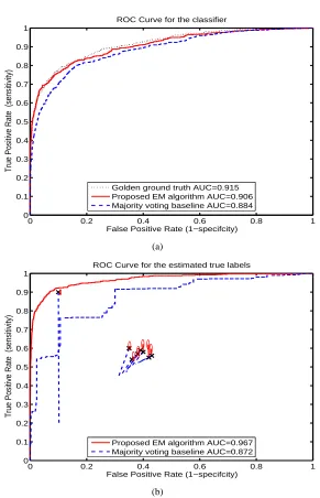
3. Actual ground truth Since the estimates of the actual ground truth are probabilistic scores, we can also plot the ROC curves of the estimated ground truth. From Figure 1(b) we can see that the ROC curve for the proposed method dominates the majority voting ROC curve. Furthermore, the area under the ROC curve (AUC) is around 3% higher. The estimate ob-tained by majority voting is closer to the novices since they form a majority (3/5). It does not have an idea of who is an expert and who is a novice. The proposed algorithm appropriately weights each radiologist based on their estimated sensitivity and specificity. The improve-ment obtained is quite large in Figure 2 which corresponds a situation where we have only one expert and 7 novices.

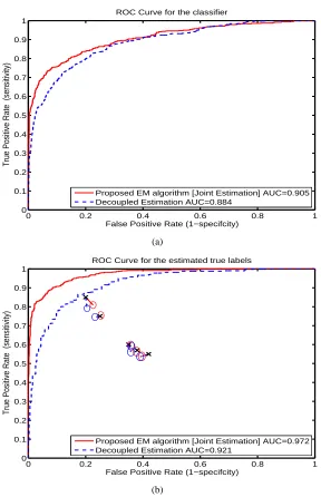
4. Joint Estimation To learn a classifier, Smyth et al. (1995) proposed to first estimate the golden ground truth and then use the probabilistic ground truth to learn a classifier. In contrast, our proposed algorithm learns the classifier and the ground truth jointly as a part of the EM algorithm. Figure 3 shows that the classifier and the ground truth learnt obtained by the proposed algorithm is superior than that obtained by other procedures which first estimates the ground truth and then learns the classifier.

6.1.2 BREASTMRI

Majority Voting True 1 True 2 True 3 True 4 True 5

Estimated 1 x 0.0217 0 x 0.0000

Estimated 2 x 0.5869 0 x 0.1785

Estimated 3 x 0.2391 0 x 0.1071

Estimated 4 x 0.1521 1 x 0.2500

Estimated 5 x 0.0000 0 x 0.4642

EM algorithm True 1 True 2 True 3 True 4 True 5

Estimated 1 x 0.0000 0 x 0.0000

Estimated 2 x 0.6957 0 x 0.1428

Estimated 3 x 0.1304 0 x 0.0000

Estimated 4 x 0.1739 1 x 0.3214

Estimated 5 x 0.0000 0 x 0.5357

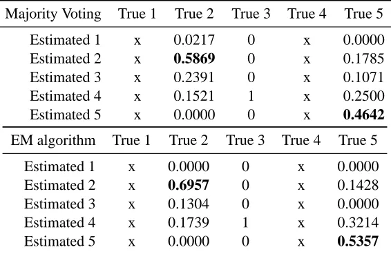
Table 1: The confusion matrix for the estimate obtained using majority voting and the proposed EM algorithm. The x indicates that there was no such category in the true labels (the gold standard). The gold-standard is obtained by the biopsy which can confirm whether it is benign (BIRADS=2) or malignant (BIRADS=5).

3 Probably Benign, 4 Suspicious abnormality, and 5 Highly suggestive of malignancy. Our data set comprises of 75 lesions with annotations from four radiologists, and the true labels from biopsy. Based on eight morphological features, we have to predict whether a lesion is malignant or not.

For the first experiment we reduce the BIRADS scale to a binary one: any lesion with a BIRADS

>3 is considered malignant and benign otherwise. The set included 28 malignant and 47 benign

lesions. Figure 4 summarizes the results. We show the leave-one-out cross validated ROC for the classifier. The cross-validated AUC of the proposed method is approximately 6% better than the majority voting baseline.

We also consider the BIRADS labels as a set of ordinal measurements since there is an order-ing among the BIRADS label. The confusion matrix in Table 1 shows that the EM algorithm is significantly superior than the majority voting in estimating the true BIRADS.

6.1.3 RECOGNIZINGTEXTUALENTAILMENT

0 0.2 0.4 0.6 0.8 1 0

0.1 0.2 0.3 0.4 0.5 0.6 0.7 0.8 0.9 1

False Positive Rate (1−specifcity)

True Positive Rate (sensitivity)

ROC Curve for the classifier

Golden ground truth AUC=0.915 Proposed EM algorithm AUC=0.913 Majority voting baseline AUC=0.882

(a)

0 0.2 0.4 0.6 0.8 1

0 0.1 0.2 0.3 0.4 0.5 0.6 0.7 0.8 0.9 1

False Positive Rate (1−specifcity)

True Positive Rate (sensitivity)

ROC Curve for the estimated true labels

Proposed EM algorithm AUC=0.991 Majority voting baseline AUC=0.962

(b)

Figure 1: Results for the digital mammography data set with annotations from 5 simulated radiol-ogists. (a) The ROC curve of the learnt classifier using the golden ground truth (dotted black line), the majority voting scheme (dashed blue line), and the proposed EM algo-rithm (solid red line). (b) The ROC curve for the estimated ground truth. The actual

sensitivity and specificity of each of the radiologists is marked as a×. The end of the

0 0.2 0.4 0.6 0.8 1 0

0.1 0.2 0.3 0.4 0.5 0.6 0.7 0.8 0.9 1

False Positive Rate (1−specifcity)

True Positive Rate (sensitivity)

ROC Curve for the classifier

Golden ground truth AUC=0.915 Proposed EM algorithm AUC=0.906 Majority voting baseline AUC=0.884

(a)

0 0.2 0.4 0.6 0.8 1

0 0.1 0.2 0.3 0.4 0.5 0.6 0.7 0.8 0.9 1

False Positive Rate (1−specifcity)

True Positive Rate (sensitivity)

ROC Curve for the estimated true labels

Proposed EM algorithm AUC=0.967 Majority voting baseline AUC=0.872

(b)

0 0.2 0.4 0.6 0.8 1 0

0.1 0.2 0.3 0.4 0.5 0.6 0.7 0.8 0.9 1

False Positive Rate (1−specifcity)

True Positive Rate (sensitivity)

ROC Curve for the classifier

Proposed EM algorithm [Joint Estimation] AUC=0.905 Decoupled Estimation AUC=0.884

(a)

0 0.2 0.4 0.6 0.8 1

0 0.1 0.2 0.3 0.4 0.5 0.6 0.7 0.8 0.9 1

False Positive Rate (1−specifcity)

True Positive Rate (sensitivity)

ROC Curve for the estimated true labels

Proposed EM algorithm [Joint Estimation] AUC=0.972 Decoupled Estimation AUC=0.921

(b)

Figure 3: ROC curves comparing the proposed algorithm (solid red line) with the Decoupled

Esti-mation procedure (dotted blue line), which refers to the algorithm where the ground truth

0 0.2 0.4 0.6 0.8 1 0

0.1 0.2 0.3 0.4 0.5 0.6 0.7 0.8 0.9 1

False Positive Rate (1−specifcity)

True Positive Rate (sensitivity)

Leave−One−Out ROC Curve for the classifier

Golden ground truth AUC=0.909 Majority voting baseline AUC=0.828 Proposed EM algorithm AUC=0.879

(a)

0 0.2 0.4 0.6 0.8 1

0 0.1 0.2 0.3 0.4 0.5 0.6 0.7 0.8 0.9 1

False Positive Rate (1−specifcity)

True Positive Rate (sensitivity)

ROC Curve for the estimated true labels

Proposed EM algorithm AUC=0.944 Majority voting baseline AUC=0.937

(b)

20 40 60 80 100 120 140 160 0.5

0.55 0.6 0.65 0.7 0.75 0.8 0.85 0.9 0.95

Number of Annotators

Accuracy

Majority Voting EM Algorithm

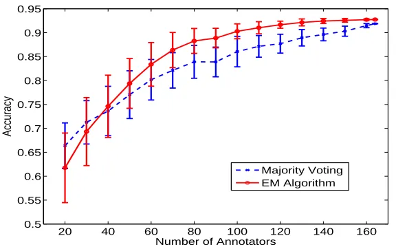
Figure 5: The mean and the one standard deviation error bars for the accuracy of the estimated ground truth for the Recognizing Textual Entailment task as a function of the number of annotators. The plot was generated by randomly sampling the annotators 100 times.

6.2 Regression Experiments

We first illustrate the algorithm on a toy dataset and then present a case study for automated polyp measurements.

6.2.1 ILLUSTRATION

Figure 6 illustrates the the proposed algorithm for regression on a one-dimensional toy data set with

three annotators. The actual regression model (shown as a blue dotted line) is given by y=5x−2.

We simulate 20 samples from three annotators with precisions 0.01, 0.1, and 1.0. The data are shown by the annotators’s number. While we can fit a regression model using each annotators’s response, we see that only the model for annotator three (with highest precision) is close to the true regression model. The green dashed line shows the model learnt using the average response from all the three annotators. The red line shows the model learnt by the proposed algorithm.

6.2.2 AUTOMATED POLYP MEASUREMENTS

0 0.1 0.2 0.3 0.4 0.5 0.6 0.7 0.8 0.9 1 −5 −4 −3 −2 −1 0 1 2 3 4 5 x (feature) y (response)

N=50 examples R=3 annotators

1 1 1 1 1 1 1 1 1 1 1 1 1 1 1 1 1 1 1 1 1 1 1 2 2 2 2 2 2 2 2 2 2 2 2 2 2 2 2 2 2 2 2 2 2 2 2 2 2 2 2 2 2 2 2 2 2 2 2 2 2 2 2 2 2 2 2 2 2 2 2 2 2 3 3 3 3 3 3 3 3 3 3 3 3 3 3 3 3 3 3 3 3 3 3 3 3 3 3 3 3 3 3 3 3 3 3 3 3 3 3

3 3 3

3 3 3 3 3 3 3 3 3 Actual regression model

Model with annotator 1 (Precision=0.01) Model with annotator 2 (Precision=0.10) Model with annotator 3 (Precision=1.00) Model with average response Proposed algorithm

Figure 6: Illustration of the proposed algorithm on a one-dimensional toy data set. The actual

regression model (shown as a blue dotted line) is given by y=5x−2. We simulate 50

samples from three annotators with precisions 0.01, 0.1, and 1.0. The data are shown by the annotators’s number. While we can fit a regression model using each annotators’s response, we see that only the model for annotator three (with highest precision) is close to the true regression model. The green dashed line shows the model learnt using the average response from all the three annotators. The red line shows the model learnt by the proposed algorithm.

0 5 10 15

0 5 10 15

Actual Polyp Diameter (mm)

Estimated Polyp Diameter (mm)

Pearson Correlation Coefficient=0.714720 RMSE=1.970815

(a) Gold standard model

0 5 10 15

0 5 10 15

Actual Polyp Diameter (mm)

Estimated Polyp Diameter (mm)

Pearson Correlation Coefficient=0.706558 RMSE=1.991576

(b) Proposed model

0 5 10 15

0 5 10 15

Actual Polyp Diameter (mm)

Estimated Polyp Diameter (mm)

Pearson Correlation Coefficient=0.554966 RMSE=2.887740

(c) Average model

We use a proprietary data set containing 393 examples (which point to 285 distinct polyps— the segmentation algorithms generally return multiple marks on the same polyp.) along with the measured diameter (ranging from 2mm to 15mm) as our training set. Each example is described by a set of 60 morphological features which are correlated to the diameter of the polyp. In order to validate the feasibility of our proposed algorithm, we simulate five radiologists according to the

noisy model described in § 5.1 withτ= [0.001 0.01 0.1 1 10]. This corresponds to a situation where

the first three radiologists are extremely noisy and the last two are quite accurate. Based on the measurements from multiple radiologists, we can simultaneously (1) learn a linear regressor and (2) estimate the precision of each radiologist. We compare the results with the classifier trained using the actual golden ground truth as well as the regressor learnt using the average of the radiologists measurements. The results are validated on an independent test set containing 397 examples (which point to 298 distinct polyps).

Figure 7 shows the scatter plot of the actual polyp diameter vs the diameter predicted by the three different models. We compare the performance based on the root mean squared error (RMSE) and also the Pearson’s correlation coefficient. The regressor learnt using the proposed iterative algorithm (Figure 7(b)) is almost as good as the one learnt using the golden ground truth (Figure 7(a)). The correlation coefficient for the proposed algorithm is significantly larger than that learnt using the average of the radiologists response. The estimate obtained by averaging is closer to the novices since they form a majority (3/5). The proposed algorithm appropriately weights each radiologist based on their estimated precisions.

7. Conclusions and Future Work

In this paper we proposed a probabilistic framework for supervised learning with multiple annota-tors providing labels but no absolute gold standard. The proposed algorithm iteratively establishes a particular gold standard, measures the performance of the annotators given that gold standard, and then refines the gold standard based on the performance measures. We specifically discussed binary/categorical/ordinal classification and regression problems.

We made two key assumptions: (1) the performance of each annotator does not depend on the feature vector for a given instance and (2) conditional on the truth the experts are independent, that is, they make their errors independently. As we pointed out earlier these assumptions are not true in practice. The annotator performance depends on the instance he is labeling and there is some degree of correlation among the annotators. We briefly discuss some strategies to relax these two assumptions.

7.1 Instance Difficulty

One drawback of the current model is that it doesn’t estimate difficulty of items. It is often observed that for the easy instances all the annotators agree on the labels—thus violating our conditional independence assumption. The difficulty of annotating an item can be captured by another latent

variableγi for each instance—which modulates the annotators performance. Models for this have

pro-posed model for sensitivity and specificity can be extended as follows (in place of (1) and (2)):

αj_(γ

i):=Pr[yij=1|yi=1,γi] =σ(aj1+bj1γi).

βj_(γ

i):=Pr[y_ij=0|yi=0,γi] =σ(aj0+bj0γi).

Here the parameters aj1 and aj0 are related to the sensitivity and specificity of the jth annotator,

while the latent termγi captures the difficulty of the instance. The key assumption here is that the

annotators are independent conditional on both yi andγi. Various assumptions can be made on two

parameters bj1 and bj0 to simplify these models further—for example we could set bj1=b1 and

bj0=b0for all the annotators.

7.2 Annotators Actually Look at the Data

In our model we made the assumption that the sensitivityαjand the specificityβjof the jth

annota-tor does not depend on the feature vecannota-torxi. For example, in the CAD domain, this meant that the

radiologist’s performance is consistent across different sub-groups of data—which is not entirely true. It is known that some radiologists are good at detecting certain kinds of malignant lesions based on their training and experience. We can extend the previous model such that the sensitivity

and the specificity depends on the feature vectorxi explicitly as follows

αj_(γ

i,xi):=Pr[yij=1|yi=1,γi,xi] =σ(aj1+bj1γi+wαj

⊤

xi).

αj_(γ

i,xi):=Pr[yij=0|yi=0,γi,xi] =σ(aj0+bj0γi+w_βj

⊤

xi).

However this change increases the number of parameters to be learned.

References

P. S. Albert and L. E. Dodd. A cautionary note on the robustness of latent class models for estimating diagnostic error without a gold standard. Biometrics, 60:427–435, 2004.

F. B. Baker and S. Kim. Item Response Theory: Parameter Estimation Techniques. CRC Press, 2 edition, 2004.

B. Carpenter. Multilevel bayesian models of categorical data annotation. Technical Report available at http://lingpipe-blog.com/lingpipe-white-papers/, 2008.

S. R. Cholleti, S. A. Goldman, A. Blum, D. G. Politte, and S. Don. Veritas: Combining expert opinions without labeled data. In Proceedings of the 2008 20th IEEE international Conference

on Tools with Artificial intelligence, 2008.

A. P. Dawid and A. M. Skene. Maximum likeihood estimation of observer error-rates using the EM algorithm. Applied Statistics, 28(1):20–28, 1979.

O. Dekel and O. Shamir. Vox Populi: Collecting high-quality labels from a crowd. In COLT 2009:

Proceedings of the 22nd Annual Conference on Learning Theory, 2009a.

O. Dekel and O. Shamir. Good learners for evil teachers. In ICML 2009: Proceedings of the 26th

A. P. Dempster, N. M. Laird, and D. B. Rubin. Maximum likelihood from incomplete data via the EM algorithm. Journal of the Royal Statistical Society: Series B, 39(1):1–38, 1977.

P. Donmez, J. G. Carbonell, and J. Schneider. Efficiently learning the accuracy of labeling sources for selective sampling. In KDD 2009: Proceedings of the 15th ACM SIGKDD international

conference on Knowledge discovery and data mining, pages 259–268, 2009.

E. Frank and M. Hall. A simple approach to ordinal classification. Lecture Notes in Computer

Science, pages 145–156, 2001.

G. Fung, B. Krishnapuram, J. Bi, M. Dundar, V. C. Raykar, S. Yu, R. Rosales, S. Krishnan, and R. B. Rao. Mining medical images. In Fifteenth Annual SIGKDD International Conference

on Knowledge Discovery and Data Mining: Third Workshop on Data Mining Case Studies and Practice Prize, 2009.

J. Howe. Crowd sourcing: Why the Power of the Crowd Is Driving the Future of Business. 2008.

S. L. Hui and S. D. Walter. Estimating the error rates of diagnostic tests. Biometrics, 36:167–171, 1980.

S. L. Hui and X. H. Zhou. Evaluation of diagnostic tests without gold standards. Statistical Methods

in Medical Research, 7:354–370, 1998.

R. Jin and Z. Ghahramani. Learning with multiple labels. In Advances in Neural Information

Processing Systems 15, pages 897–904. 2003.

B. Krishnapuram, J. Stoeckel, V. C. Raykar, R. B. Rao, P. Bamberger, E. Ratner, N. Merlet, I. Stain-vas, M. Abramov, and A. Manevitch. Multiple-instance learning improves CAD detection of masses in digital mammography. In IWDM 2008: Proceedings of the 9th international workshop

on Digital Mammography, pages 350–357. 2008.

G. Lugosi. Learning with an unreliable teacher. Pattern Recognition, 25(1):79–87, 1992.

R. M. Neal and G. E. Hinton. A view of the EM algorithm that justifies incremental, sparse, and other variants. In Learning in Graphical Models, pages 355–368. Kluwer Academic Publishers, 1998.

V. C. Raykar, S. Yu, L .H. Zhao, A. Jerebko, C. Florin, G. H. Valadez, L. Bogoni, and L. Moy. Supervised learning from multiple experts: Whom to trust when everyone lies a bit. In ICML

2009: Proceedings of the 26th International Conference on Machine Learning, pages 889–896,

2009.

V. S. Sheng, F. Provost, and P. G. Ipeirotis. Get another label? improving data quality and data mining using multiple, noisy labelers. In Proceedings of the 14th ACM SIGKDD International

Conference on Knowledge Discovery and Data Mining, pages 614–622, 2008.

P. Smyth. Learning with probabilistic supervision. In Computational Learning Theory and Natural

P. Smyth, U. Fayyad, M. Burl, P. Perona, and P. Baldi. Inferring ground truth from subjective labelling of venus images. In Advances in Neural Information Processing Systems 7, pages 1085– 1092. 1995.

R. Snow, B. O’Connor, D. Jurafsky, and A. Ng. Cheap and fast - But is it good? Evaluating non-expert annotations for natural language tasks. In Proceedings of the Conference on Empirical

Methods in Natural Language Processing, pages 254–263, 2008.

A. Sorokin and D. Forsyth. Utility data annotation with Amazon Mechanical Turk. In Proceedings

of the First IEEE Workshop on Internet Vision at CVPR 08, pages 1–8, 2008.

J. S. Uebersax and W. M. Grove. A latent trait finite mixture model for the analysis of rating agreement. Biometrics, 49:823–835, 1993.

S. K. Warfield, K. H. Zou, and W. M. Wells. Simultaneous truth and performance level estimation (STAPLE): an algorithm for the validation of image segmentation. IEEE Transactions on Medical

Imaging, 23(7):903–921, 2004.

J. Whitehill, P. Ruvolo, T. Wu, J. Bergsma, and J. Movellan. Whose vote should count more: Opti-mal integration of labels from labelers of unknown expertise. In Advances in Neural Information