Prediction of Pressure Gradient in Two and Three-Phase Flows in
Vertical Pipes Using an Artificial Neural Network Model
Joseph Xavier Francisco Ribeiro
1,2,3,*, Ruiquan Liao
1,2, Aliyu Musa Aliyu
4, Zilong Liu
1,21Petroleum Engineering College, Yangtze University, Wuhan Hubei, China
2Laboratory of Multiphase Flow, Gas Lift Innovation Centre, China National Petroleum Corporation, China
3Kumasi Technical University, P. O. Box 854, Kumasi, Ghana
4
Faculty of Engineering, University of Nottingham, NG7 2RD, United Kingdom
Received 14 January 2019; received in revised form 23 February 2019; accepted 13 March 2019
Abstract
The concurrent flow of gas with a mixture of oil and water is often observed in production tubing in the
petroleum industry. Lack of physical understanding of the several phenomenological characteristics of three-phase
flow can lead to unsatisfactory production rates or even oversizing of pipelines. Additional investigations to gain
more insight and development of more accurate correlations for prediction of flow characteristics including
pressure drop is necessary. In this study, an experimental study was conducted using air-water and air-water-oil
mixtures in a 0.075m diameter pipe. Superficial gas and liquid velocities ranged from 0.03 to 0.13 m/s and 1.26 to
41.58 m/s respectively. Slug flow was the main flow pattern observed. In addition, the transition from churn to
annular flow and annular were also observed. Due to the homogeneous nature of the oil-water-air mixture, the
three-phase flow was evaluated as a pseudo-two-phase mixture. An Artificial Neural Network (ANN) model
developed for the prediction of two-phase and three-phase pressure drop performed better than all models
considered during the evaluation. Generally, it was found that the accuracies for pressure drop were considered
adequate.
Keywords: artificial neural networks, two-phase flow, three-phase flow, pressure drop, vertical pipes
1.
Introduction
Simultaneous flow of gas and oil-water mixtures are common in production equipment found in the chemical industry,
pipelines in the petroleum industry and also in various installations in the food industry [1]. Water fraction in the liquid
phase can be in excess of 90% in numerous cases in the transportation pipelines in the petroleum industry [2]. Water
injection in the reservoir to enhance production as part of enhanced oil recovery processes [3] among other tangible reasons
can generate this phenomenon. The resulting three-phase flow may influence flow characteristics [4].
The pressure gradient is an essential characteristic of multiphase flow and is well connected to the estimation of other
critical flow hydrodynamic parameters of inducts including void fraction [1]. Proper prediction of the pressure gradient is
critical to enhancing production tubing design in the oil industry. Therefore, accurate prediction of pressure gradient would
lead to improved safety in operations and performance of equipment and also higher returns on investment.
The effect of three-flow characteristics in conduits differs significantly from that of two-phase flow. Comparatively,
research efforts aimed at predicting pressure gradient in conduits have focused more on two-phase flows despite the
occurrence of three-phase flows in industry. Though research efforts have been made by several authors [1, 5-12], additional
attention must be paid to the behavior and characteristics of three-phase flows in conduits through the contribution of data
obtained from experimental studies as these may have a direct impact on pumping requirements and hence profitability.
Furthermore, continued validation of existing prediction models and methods is necessary to enhance confidence in their
capabilities and identify flaws for improvement.
Improving the accuracy of pressure gradient predictions remain a major thrust for multiphase flow research and
correlation development for flow parameters. Inherent complexities associated with varied phase distributions and a wide
range of fluid properties encountered during production operations present challenges to the development of accurate
correlations for pressure gradient predictions [13]. In summary, machine learning techniques and ANN, in particular, have
been employed by some researchers to provide alternative prediction solutions for two-phase flow parameters including
liquid holdup, pressure gradient and gas void fraction with success [13-16], however, we note that their use for three-phase
flows is not reported in the open literature.
2.
Previous Work
[16] employed neural networks to predict holdup and flow pattern in pipes under various angles of inclinations. They
developed neural network models based on experimental data limited to a 1.5-inch (38.1 mm) pipe and low operating
pressures. They utilized a Kohonen-type network to classify the four different correlations for flow patterns with all input
data. The resulting classifications from the output layer in binary form were used as data input to a three-layer
backpropagation neural network for predicting holdup. Holdup values predicted by the neural network had a coefficient of
determination(R2) value of 0.945. This showed an improvement in prediction when compared with Mukherjee’s result of
0.904.
[17] presented two Artificial Neural Networks (ANN) models capable of identifying the flow regimes and also
calculating liquid holdup in the horizontal and near horizontal gas-liquid multiphase flow respectively. The published
experimental data employed consisted of 111 data points from Minami and Brill who utilized water as well as
air-kerosene mixtures and 88 data points from Abdul-Majeed who used air-air-kerosene for his experiment. Models were developed
using a three-layer feedforward backprop neural network. Superficial gas and liquid velocities, pressure, temperature and
fluid properties were used as inputs to the network. The outputs of the first and second networks were flowed regime and
liquid holdup respectively. Their results showed that the developed models provide better predictions and have higher
accuracy than the empirical correlations (developed specifically for these data groups). The developed flow regime model
predicted the flow regime correctly for more than 97% of the data points. The ANN liquid holdup model outperformed
published models in terms of the lowest standard deviation (8.544) and the highest correlation coefficient (0.9896).
[13] obtained experimental data from Eaton (128 data points, water-natural gas; 110 data points, water-natural gas),
Beggs (30 data points, water-air; 28 data points, water-air), Mukherjee (74 data points, kerosene-air; 57 data points, lube
oil-air), Minami and Brill (57 data points, air; 54 data points, water-oil-air), and Abdul-Majeed (89 data points,
kerosene-air) respectively and trained a Multi-Layer Perceptron (MLP) neural network with 7 input variables (pipe diameter,
superficial velocity of liquid, superficial velocity of gas, viscosity, surface tension and no-slip liquid holdup) to predict liquid
holdup for horizontal gas-liquid two-phase flows. The holdup values predicted by their neural network had a correlation
coefficient (R) of 0.985 for all data sets. Evaluation of the ANN model showed a better performance than all models with
which it was compared.
Recently, [14-15] have applied ANN to predict void fraction data for gas-liquid flow in horizontal, upward and
downward inclined pipes, the pressure gradient in horizontal oil-water separated flow and water holdup in vertical and
3.
Methodology
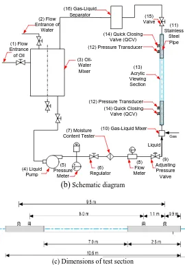
3.1. Description of flow facility
The experiment was implemented on a test rig capable of inclinations from 0-90° (Fig. 1) at the Gas Lift Innovation
Centre, Yangtze University, China. For two-phase flow, the desired volume of oil was pumped into a mixing tank, and
pressurized. After pressure stabilization and measurement, the liquid is mixed with compressed gas and introduced into the
test section. The liquid returns to the mixing tank while the air is released into the atmosphere after the gas-liquid mixture
has passed through the separator. For three-phase flow, liquid and water were pumped into the mixer, stirred continuously
till a homogeneous mixture is achieved, mixed with gas and introduced into the test section.
(a)
Photo of the experimental rig in vertical positionL B
P B
Gas
Liquid (3)
Oil-Water Mixer (16) Gas-Liquid
Separator
(14) Quick Closing Valve (QCV)
(15) Valve
(9) Adjusting Pressure Valve (14) Quick Closing
Valve (QCV) (12) Pressure Transducer
(10) Gas-Liquid Mixer
(11) Stainless
Steel Pipe
(13) Acrylic Viewing Section
(12) Pressure Transducer
(4) Liquid Pump
(7) Moisture Content Tester (2) Flow
Entrance of Water
(1) Flow Entrance of Oil
(8) Flow Meter (6)
Regulator (5)
Pressure Meter
(b)
Schematic diagram(c) Dimensions of test section
The acrylic test section (Fig. 1) is a pipe of length 10.6 m and an ID of 0.075 m. The viewing section consists of an
acrylic tube with a length of 7 m. Stainless steel pipes of lengths 1.1 m and 2.5 m respectively are fixed at each end of the
acrylic tube. Pressure, temperature, and pressure differential sensors, as well as quick closing valves and other devices, are
installed on the pipe section. The distance between the two quick closing valves is 9.5 m. The distance between the
differential pressure transducers is 8 m. The temperature of the two-phase and three-phase mixtures was determined using a
type K thermocouple. Similar test section arrangement has been employed by [18-19] for their studies. Control of the devices,
as well as data collection, is done directly online at an established control center. Details of the measuring equipment utilized
for the experiment are presented in Table 1. Air constituted the gas phase while oil and an oil-water mixture respectively
were used as the liquid phase. The fluid properties are presented in Table 2.
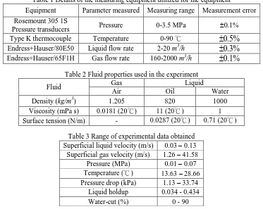
Table 1 Details of the measuring equipment utilized for the equipment
Equipment Parameter measured Measuring range Measurement error
Rosemount 305 1S
Pressure transducers Pressure 0-3.5 MPa 0.1%
Type K thermocouple Temperature 0-90 ℃
0.5%
Endress+Hauser/80E50 Liquid flow rate 2-20 m3/h
0.3%
Endress+Hauser/65F1H Gas flow rate 160-2000 m3/h
0.1%
Table 2 Fluid properties used in the experiment
Fluid Gas Liquid
Air Oil Water
Density (kg/m3) 1.205 820 1000
Viscosity (mPa s) 0.0181 (20℃) 11 (20℃) 1 Surface tension (N/m) - 0.0287 (20℃) 0.71 (20℃)
Table 3 Range of experimental data obtained Superficial liquid velocity (m/s) 0.03 – 0.13
Superficial gas velocity (m/s) 1.26 – 41.58 Pressure (MPa) 0.01 – 0.07 Temperature (℃) 13.63 – 28.66 Pressure drop (kPa) 1.13 – 33.74
Liquid holdup 0.034 - 0.434
Water-cut (%) 0 - 90
3.2. Experimental procedure and measurement
For this study, a constant liquid flow rate was maintained, while the gas flow rate was adjusted. When the system was
deemed steady (approximately 10 minutes from the start of the experiment), the experimental flow pattern was observed and
recorded. Except for liquid holdup, all other experimental data was recorded every 5 seconds for 3 minutes, and finally, the
average value of each measurement parameter was obtained. Each complete test took approximately 20 minutes depending
on the time required to reach steady-state. After the data recording was completed, the quick closing valve was closed
trapping fluids flowing in the test section. The liquid holdups were measured by using a 9 m longitudinal pipe section. The
quick closing valve has a response time is 0.3-0.5s. The trapped oil-water-air mixture was allowed to settle for 5 minutes and
the pipe raised to facilitate draining of the liquid into a measuring cylinder. The liquid holdup was determined by calculating
the volume of the liquid and dividing it by the volume of pipe-section. Flow patterns were visualized directly and also
observed using a Canon Xtra NX4-S1 high-speed camera capable with a pixel resolution of 1024x1024 up to 3000 frames
per second (fps). The maximum frame rate is 50,000 fps with a reduced resolution. Videos and pictures of the flow pattern
were obtained and used for analysis during the study. The range of measurements taken during the experiments is presented
in Table 4.
Fully developed flow is a key required for multiphase studies. For this experiment, fully developed flow was observed
pipes have been observed at lower L/D values by a number of researchers including. For slug flows, Taitel et al. [20]
theoretically estimated minimum value of 50 for fully developed slug flow. [21] achieved a fully developed an annular flow
with L/D=59-92. [22-24] demonstrated that an L/D=46 is sufficient for annular flow. [25] also showed that an L/D of 41 is
sufficient for such experiments. It can be assumed, therefore, that this represents a sufficient flow development length for
both slug and the annular flows observed in this study.
4.
Results and Discussions
4.1. Comparison with existing flow pattern maps
Fig. 2 shows pictures of flow patterns observed at different conditions during the experiment. For both two-phase and
three-phase flows, slug flow, the transition to annular flow, and annular flows were observed. However, slug flow
constituted the main flow pattern observed. There were no apparent differences between the flow patterns observed for
two-phase and three and two-phase flows.
(a) Slug flow at vsl=0.03 m/s, vsg=1.34 m/s, water-cut=60%
(b) Transition to annular flow m/s, vsl=0.04, vsg=11.63m/s, water-cut=60%
(c) Annular flow vsl=0.1m/s, vsg=38.63m/s, water-cut=60%
Fig. 2 Flow patterns observed at various flow conditions during the experiment
Three existing flow pattern maps were validated using the experimental data. To achieve this, the experimental data
points corresponding to the flow regimes were superimposed on the flow pattern maps [20, 22, 26] (Fig. 3). It is observed
that the map [20] captures the behavior of the two-phase and three-phase experimental flow patterns. Though the flow
pattern map is developed based on data using air-water (1 mPa s) mixtures and a pipe diameter of 50 mm, both of which are
lower than what was applied in the experiment, the observation agrees with proposed mechanisms for flow pattern transition.
The flow pattern map [26] incorporates the effects of flow rates, fluid properties, pipe configuration, and angle of inclination.
It is found that the flow pattern map also agrees with both the experimental data. Considering that the efficacy of this flow
pattern map is already proven, the current observation perhaps provides an indication of its efficiency for three-phase flow
pattern prediction. When the experimental data is plotted on the Shell flow pattern map [22], it is observed that it fairly
agrees with the two-phase flow data. A similar conclusion can be made when the three-phase data is imposed on it. The
discrepancies can be attributed to the differences in pipe diameter, liquid and gas densities as well as liquid viscosities. The
experimental data for phase densities and pipe diameter are lower than those employed for the development of the flow
(a) Taitel et al. flow pattern map
(c) Shell flow pattern map (b) Barnea flow pattern map
Fig. 3 Comparison of experimental flow pattern data with existing flow pattern maps
4.2. Total pressure drop
The total pressure drop was measured with a differential pressure transducer (DP cell). The separation distance between
the DP cell was 8 m. The variation of total pressure drop with superficial gas velocity for 0% to 90% water-cut is presented
in Fig. 4. Some slight differences were observed between two- and three-phase flows. High values of pressure drop in the
three-phase flow were observed compared to that of two-phase air-oil flow. The total pressure gradient is composed of
gravitational and friction pressure gradients. At low superficial phase velocities, compared to the that of the air-oil mixture
density, higher water-cut introduces higher values of mixture density which increases the gravity component and hence the
total pressure gradient [6, 27]. At vsl < 0.08 m/s, the total pressure gradient is observed to decrease with increasing superficial gas velocity. The observation can be explained by the fact that flow is gravity dominated as is the case in vertical
pipes. An increase in superficial gas velocity promotes an increase in a void fraction, which in turn, reduces the mixture
density as a consequence of decreases in liquid holdup [1]. Also, at low vsg values, the gas velocities are not high enough to
generate high friction pressure drops, hence the total pressure drop decreases with increases in superficial gas velocity. All
points within this range are observed to be in the slug flow regime.
At vsl ≥ 0.08 m/s, it is observed that total pressure drop decreases to a minimum and then begins to increase again.
Decreases in the gravitational pressure gradient (because of reduction in total liquid holdup) as well as in the friction
pressure drop consequently leads to a cumulative decrease in total pressure drop (Fig. 4). The minimum point represents a
condition where the frictional pressure drop overcomes the gravitational pressure drop as the superficial gas flow rate is
increased. This point always terminates in slug flow and also marks the transition from slug flow to churn and then to
annular flows where friction pressure drops are higher due to the cumulative effect of interfacial friction between gas and
1 10
1E-3 0.01 0.1 1 10
Finely Dispersed
Slug or Churn
Le/D = 100 200
Vsl
(m
/s)
Vsg (m/s)
0% slug flow
0% transition to annular 0% annular flow 90% slug flow
90% transition to annular flow
500 Slug
Bubble flow
flow
Annular flow
0.01 0.1 1 10
1E-5 1E-4 1E-3 0.01 0.1
0%, slug flow
0% transition to annular 0% annular flow 90% slug flow
90% transition to annular flow
Frl
(
- )
Frg ( - )
Mist flow Annular flow
Intermittent flow
1 10 100
1E-3 0.01 0.1 1 10
0%, slug flow 0% tranistion to annular 0% annular flow 90% slug flow 90% transition to annular
Vsl
(m
/s)
Vsg (m/s) Dispersed bubble
Intermittent
liquid and also the liquid and the conduit wall. The observation has previously been reported by [28] whose experimental
studies utilized liquids of high viscosities and a pipe ID of 50 mm observed and reported only one minimum. In this study,
only one minimum was observed in both two-phase and three-phase flows for the superficial gas velocity range studied.
While this phenomenon is well-noted for two-phase gas-liquid flows, it is shown in this work that it can also be exhibited in
the three-phase flows when the oil-water mixtures are homogeneously mixed. This provides credence to the approach which
considers three-phase flow as pseudo-two-phase flows for multiphase flow analyses.
For this study, superficial liquid velocity appeared to have some influence at visible at low vsl and vsg values, especially at 0% and 30% water-cut. However, it is observed that the phenomenon is inconsistent across all water-cuts. It is
concluded, therefore, that the influence of superficial liquid velocity is negligible at low vsg and vsg values.
(a) 0% water-cut (b) 30% water-cut
(c) 60% water-cut (d) 90% water-cut
Fig. 4 Variation of total pressure drop with superficial gas velocity
When vsl < 0.08 m/s and 5 m/s < vsg < 15 m/s, however, it is observed that increases in vsg values lead to increases in
total pressure drop. This can mainly be because of the increased gravitational pressure drop. The intermittent flow is
preferred in the production of oil and gas in vertical wells, especially when the gas lift is used because the minimum total
pressure gradient occurs under intermittent-flow condition. Gas lift is preferred under intermittent-flow conditions because it
reduces the liquid holdup, causing a reduction in gravitational- pressure and total pressure drops in the tubing and leading to
a more stable flow. On the basis of this observation, it implies gas-lift can be applied to both the two-phase and three-phase
flows within the viscosity ranges in this study but not at higher viscosities since they tend to shift the minimum pressure drop
to higher values, leading to less favorable flow conditions.
Finally, water-cut exerts some influence between two-phase and three-phase flows. As earlier stated, the differences in
values of total pressure gradient can be attributable to differences in mixture density in the three-phase flow as a result of
increasing water fraction which increases the hydrostatic pressure gradient and hence the total pressure gradient.
0 10 20 30 40
0 5 10 15 20 25 30 35 V
sg (m/s)
T ot al Pres s ure D rop (k Pa) V sl=0.03m/s V sl=0.08m/s V sl=0.13m/s
0 10 20 30 40
0 5 10 15 20 25 30 35 V
sg (m/s)
T ot al Pres s ure D rop (k Pa) V sl=0.03m/s V sl=0.08m/s V sl=0.13m/s
0 10 20 30 40
0 5 10 15 20 25 30 35 V
sg (m/s)
T ot al Pres s ure D rop (k Pa)
Vsl=0.03m/s V
sl=0.08m/s
Vsl=0.13m/s
0 10 20 30 40
5 10 15 20 25 30 35 V
sg (m/s)
T ot al Pres s ure D rop (k Pa)
Vsl=0.03m/s V
sl=0.08m/s
5.
Description of ANN Model
Artificial Neural Networks (ANN) consist of numerous simple interconnected elements known as neurons which mimic
the functions of biological neurons. The neurons are organized in layers and tied together with weighted connections
corresponding to human brain synapses [14]. ANNs are capable of learning, storing and recalling information based on a
given training dataset and provide an unconventional approach for many engineering problems that are difficult to describe
or solve using normal methods [29]. Other important benefits are reported by [14].
Artificial neural networks have an input layer, output layer and can have one or more hidden layers. Each layer contains
a weight matrix (w) and a bias vector. The Feed Forward Back Propagation (FFBP) network is one of the common networks
employed to model approximate function problems. The mechanism of operation employed by this network is adequately
described by [14-15]. A three-layer MLP network has been mathematically proven to be capable to approximate all types of
functions with no consideration of their complexities [30].
Transfer functions applied in neural networks include linear (purelin), hyperbolic tangent sigmoid (tansig), logarithmic
sigmoid (logsig) and radial basis (radbas) transfer functions. The most popular of these applied to non-linear relationships
are the tansig and logsig transfer functions which produce output values in the ranges of [-1,1] and [0,1] respectively.
General forms of the functions are expressed in Eqs. (1) and (2) respectively [14-15].
Hyperbolic tangent sigmoid (tansig):
j j
j j
s s
j s s
f
S
e
e
e
e
(1)Logarithmic sigmoid (logsig):
1
j j
j S S
f
S
e
e
(2)where f(Sj) is the output of the node j and is also the element of the inputs to the nodes of the next layer. During training, the
network “learns” and develops the relationship between the data provided using an algorithm to modify the weights based on
the error between the actual values (also known as targets) and the predicted values until it generates the best relationship
between inputs and outputs (targets) given. In the FFBP network, the fitting procedure from which the weights are
determined is performed by employing the least - square minimization routine where the sum of the square of the errors
between the actual and the predicted values are minimized [14-15].
In this study, MATLAB’s neural network toolbox was employed to design networks for the prediction of liquid
holdup and pressure drop. A feed-forward with the back-propagation network architecture was selected and utilized. Though
multiple hidden layers can be utilized for a chosen network one hidden layer is usually considered adequate for modeling
non-linear and complex functions [31]. For this study, one hidden layer was adopted to obtain accurate predictions. To
identify the optimal model, both tansig and logsig transfer functions were utilized in the hidden layer of the Feed Forward
Back Propagation (FFBP) networks. Also, for both networks, a linear transfer function was utilized for the output layer
neurons. A schematic representation of the ANN architecture for the proposed network, with 13 neurons, in the study is
shown in Figure 5. Efforts were made to improve network performance by eliminating unnecessary input variables to placate
the curse of dimensionality [32]. To this end, a 112-point data set was obtained from the multiphase flow database at the
multiphase flow laboratory of Yangtze University as described in section 2.
Using the data, commonly used dimensionless multiphase flow parameters including liquid number, gas velocity
number, liquid velocity number, gas Reynolds number, liquid Reynolds number, liquid viscosity number, and mixture
velocity Froude number were determined. Selection of input parameters was based on correlation coefficients and p-values
when they were correlated with liquid holdup and pressure drop to determine their significance. Finally, the superficial gas
overflows due to the application of very small or very large weights, input data was scaled to a range of [-1,1] [33]. The
related expressions for the input parameters are as follows: the gas velocity number,Ngv=vsg(ρl/gσl)0.25, Superficial gas
Reynolds number, ReSG=ρgvsgD/μg, and the Mixture velocity Froude number, Fr=vm/(gD)
0.25
; where vsg, vm, ρl, ρg, μg, g, σl,
Drepresent superficial gas and mixture velocities, liquid and gas densities, gas viscosity, gravitational acceleration, surface
tension, and pipe diameter respectively.
Fig. 5 Schematic representation of the ANN architecture used in this study with 13 neurons for pressure drop
The dividend algorithm was implemented to ensure that data input parameters were randomly divided into three sets:
training, validation, and testing. The training data set is used for the development and adjustment of weights and biases of
the network. The validation set is used to ensure the accuracy of and generalization of the network during the training phase
while the testing set is used to evaluate the final performance of the trained network. For this study, 65% (73 data points)
was used for training, 15% (17 data points) for validation and 20% (22 data points) for testing.
The network was trained using the Levenberg-Marquardt (LM) algorithm which is recommended for the training of the
type of neural network selected [34] and to evaluate the method of convergence. LM was adopted due to its capacity to train
rapidly and efficiently and in addition increase the convergence speed of the ANN with MLP architectures [35]. Further, it
was chosen because it is suited to training networks in which the performance index is calculated in Mean Squared Error
(MSE) which was the case for this study.
By default, the toolbox ensures that a number of neurons in the input and output layers is equal to the number of input
and output parameters respectively. However, the number of neurons in the hidden layer differ based on the complexity of
the problem. Choice of the optimal number of neurons is usually by a trial and error method. The optimal number of neurons
for this study was estimated by minimizing the Mean Squared Error (MSE) of the testing data set based on the expression in
Eq. (3).
, Pr ,
21
1
nExp m ed m
m
MSE
Y
Y
n
(3)W1(1,j) AF M1
W1(12,j) AF M12 W1(6,j) AF M6
W1(11,j) AF M11 W1(5,j) AF M5
W1(10,j) AF M10 W1(9,j) AF M9 W1(8,j) AF M8 W1(7,j) AF M7 W1(4,j) AF M4 W1(3,j) AF M3 W1(2,j) AF M2
Input layer Hidden layer Output layer
PD
OF W2,i
b2i
b1i
Gas Velocity Number
W1(13,j) AF M13
Superficial Gas Reynolds
Number
where n is the number of data points, Y(Exp,m) is the experimental value and Y(Pred,m) is the predicted value obtained
from the neural network model. It is noteworthy to point out that the optimal number of neurons in the hidden layer, as well
as their related weights and biases, are not known at the developmental stage of the network and hence must be optimized.
To achieve this, the training process for each network was performed 200 times for each number of neurons in the hidden
layer. Eventually, the network with the best performance for testing data was selected as the optimal ANN model.
The number of neurons for each network was varied from 1-20 with several runs performed for each network with the
aim of preventing wrong selection of initial weights. Performance of the optimal model was evaluated with coefficient of
correlation (R) and Mean Absolute Percent Error (AAPE) and the chi-square test defined in Eqs. (4) to (6).
Pr , Pr ,
, Pr ,
1
2 2
, Pr ,
, Pr ,
1 1
[
]
n
ed m ed m
Exp m ed m
m
n n
Exp m ed m
Exp m ed m
m m
R
Y
Y
Y
Y
Y
Y
Y
Y
(4), Pr ,
, 1
1
100 n
Exp m ed m Exp m m
AAPE Y Y
n Y
(5)Pred m,
Y
in Eq. (5) is the average of the experimental values.
22 1 n observed predicted predicted i
Y
Y
Y
(6)Finally, for pressure drop, a logsig transfer function, 13 neurons in the hidden layer (3-13-1), an MSE of 3.34 and
AAPE of 12.32 for the testing data was obtained as the optimum model with the best performance (Table 5). The expression
for the pressure drop model is given as:
2
2 1 , 1
1 1
log
iN J
j
i i j i
i J
PD
w
sig
w
x
b
b
(7)where xj=(x1,x2,x3,…xj) T
represents the input sample. In our case, the input sample consisted of values of gas velocity number,
superficial gas Reynolds number, and mixture velocity Froude number as was used for the correlation. Pressure drop was the
linear output of the hidden neurons and an output function used on the neurons. J and N are the numbers of the input
variables and hidden nodes respectively. w1i,j and w2i represent the hidden layer and the output layer weight matrices
respectively. b1i and b2i represent the corresponding bias vectors. The values of the coefficients w1, w2, b1 and b2 are provided
in Table 4.
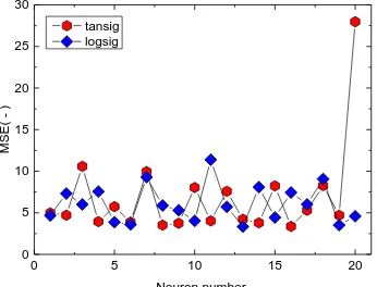
Fig. 6 Performance of the testing data for the networks using tansig and logsig transfer functions for different neuron configurations in the hidden layer for pressure drop
0 5 10 15 20
Performance of the testing data using the tansig and logsig transfer functions for different neuron configurations are
presented in Fig. 6. Performance evaluation of selected ANN model for pressure drop for training, validation, testing, and all
data sets are presented in Table 5. A chi-square test performed for the overall data for both liquid holdup and pressure
yielded a result of 1.0 respectively indicating that statistically, there is no difference between the experimental and
predictions of the ANN model.
Table 4 Weights and biases for the ANN model for total pressure drop
Input layer weight matrix
w
1j Input layer bias vector Hidden layer weight vector Output layer bias vector1
J J2 J3 b1 w2 b2
4.78675 7.36309 5.72555 19.42174 -6.62567 6.12795
-3.74608 -5.24535 1.86564 5.16499 2.94957 -
5.74774 1.37953 -4.82578 -0.94082 3.24712 -
-12.70850 13.64704 1.74692 0.35186 17.46855 -
5.53657 -0.97388 0.56158 -3.19332 -0.277974 -
-3.57842 -2.57294 -5.69732 3.76079 2.06571 -
4.49847 3.39882 1.41166 -1.34967 -1.68959 -
0.72446 -5.38652 -4.29988 -0.63222 2.87519 -
-16.54361 -25.73575 35.38188 -8.68275 -19.70100 -
4.28230 -1.55343 2.90164 2.25365 -7.39846 -
-4.50234 2.76668 3.71641 -4.62954 0.15867 -
-0.85869 6.11527 4.17686 9.60003 7.04933 -
11.46532 7.23165 -11.31631 7.72461 -17.40596 -
4.78676 7.36309 5.72555 19.42174 -6.62567
From Table 5, it can be observed that model predictions were with low Mean Squared Errors (MSE) and Average
Absolute Percent Errors (AAPE) respectively. Low MSE values were achieved for training and testing data sets respectively
for pressure drop. Generally, the MSE values calculated for all the data sets are closer to zero indicating that the model is
well fitted while the prediction errors are low. The results verify the success of the neural network to recognize the implicit
relationship between input and output variables.
Table 5 Performance evaluation of selected networks for total liquid holdup and total pressure drop
Data Total Pressure Drop
No. of data points Datasets R MSE AAPE 2
73 Training 0.9785 1.25 7.19 -
17 Validation 0.9531 2.81 10.48 -
22 Testing 0.9629 3.34 12.32 -
112 Overall 0.9629 2.61 8.70 1.0
6.
Comparison with Existing Pressure Gradient Prediction Models
The pressure gradient predictions of six empirical (Beggs and Brill, Govier and Aziz, Duns and Ros, Hagedorn and
Brown, Mukherjee and Brill, Gray) and two mechanistic (Ansari et al., Zhang et al.) models compared with the predictions
of the ANN model. PIPESIM [36], a steady-state flow simulator is utilized to obtain a prediction of the selected models.
Phase inversion defines the phenomenon which occurs when the continuous and dispersed phases invert spontaneously at
certain flow conditions [1, 37]. This phenomenon influences pressure gradient prediction especially where liquid-liquid
mixtures are involved [38]. To account for phase change in the three-phase flows, the correlation [39-40] were activated in
the simulator. The correlation [40] determined the point of phase inversion while the correlation [39] determined the
effective liquid mixture viscosity for each flow condition. The correlation [27] are expressed as:
0.6 0.4
0.6 0.4
1
1
t t o o
t t
t t w w
c
(8)
where c is the cut-off/100, μo, μw are the oil and water viscosities (cP). The correlation [39] calculates elevated emulsion
2.51
m c d
(9)where μc and Ød represent the viscosity of the continuous phase and the volume fraction of the discontinuous phase. The
results are assessed using statistical parameters AAPE and APE. The expression for APE is as follows:
, Pr ,
, 1
1
100 n
Exp m ed m Exp m m
Y Y
APE
n Y
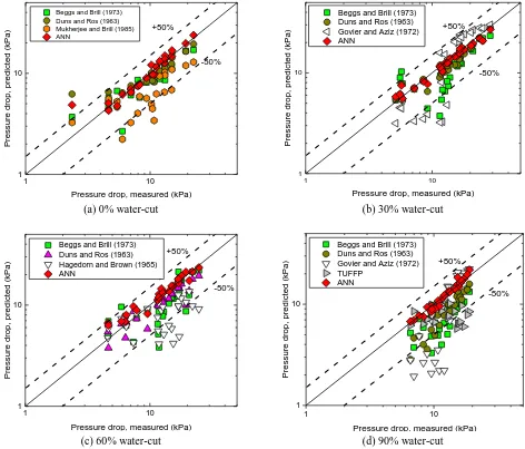
(10)Results of the assessment are presented in Table 6. In addition, a pictorial assessment of models with the best
predictions at each water-cut is presented in Fig. 7. For two-phase flow, it is found that the predictions of all the models are
satisfactory. However, the Beggs and Brill and Duns and Ros present the best and second-best performances of the models
under consideration. Comparatively, the best performance is presented by the ANN model with very low AAPE and APE
values of 11.46 and -5.78. The performance of the TUFFP model is reasonable.
(a) 0% water-cut (b) 30% water-cut
(c) 60% water-cut (d) 90% water-cut
Fig. 7 Comparison of experimental data with total pressure drop predictions of selected models
At 30% water-cut, it also observed that, with the exception of the Hagedorn and Brown’s model, all the models
under-predict the experimental data. The ANN presents the best performance, placing it ahead of all other models with low AAPE
and APE values of 6.58 and 1.95. The Duns and Ros model comes second with comparatively low AAPE and APE values of
13.27 and 9.15 respectively. This is followed by the Beggs and Brill (AAPE=29.26, APE=16.02) and the Govier and Aziz
(AAPE=32.54, APE=4.76) models. Generally, predictions of the models at this water-cut are satisfactory.
1 10
1 10
Beggs and Brill (1973) Duns and Ros (1963) Mukherjee and Brill (1985) ANN Pressu re dr op , p re dicte d ( kPa)
Pressure drop, measured (kPa) +50%
-50%
1 10
1 10
Beggs and Brill (1973) Duns and Ros (1963) Govier and Aziz (1972) ANN Pressu re dr op , p re dicte d ( kPa)
Pressure drop, measured (kPa) +50%
-50%
1 10
1 10
Beggs and Brill (1973) Duns and Ros (1963) Hagedorn and Brown (1965) ANN Pressu re dr op , p re dicte d ( kPa)
Pressure drop, measured (kPa) +50%
-50%
1 10
1 10
Beggs and Brill (1973) Duns and Ros (1963) Govier and Aziz (1972) TUFFP ANN Pressu re dr op , p re dicte d ( kPa)
Pressure drop, measured (kPa) +50%
For this experimental data, it is found that the empirical models perform better than their mechanistic counterparts at all
conditions under consideration (Table 6). The performance of the mechanistic models not was expected. Though both
considered models capture the dynamics of the flow differently, it seems that adopted closure models, some of which are
derived from air-water two-phase flows and air-oil mixtures of lower viscosities, limit their performances. Improved closure
relationships could greatly improve model predictions. The performance of the ANN was also expected because of its
superior abilities at generating good expressions for even the most complex relationships.
Table 6 Performance evaluation of all models for pressure drop at 0%, 30%, 60% and 90% water-cuts respectively
Two-phase Three-phase
Overall
0% 30% 60% 90%
AAPE APE AAPE APE AAPE APE AAPE APE AAPE APE
Empirical
BB 18.64 7.38 29.26 16.02 27.83 15.44 38.48 38.36 27.98 19.49
DR 19.45 -1.87 13.27 9.15 16.39 12.21 33.06 33.06 20.01 13.76
GA 34.73 -6.09 32.54 4.76 40.54 -0.42 35.12 22.45 34.76 5.92
Gray 53.34 50.22 51.80 46.35 48.03 34.46 53.19 49.92 49.21 43.10
HBR 45.36 3.95 49.16 -10.71 37.33 31.53 56.24 56.24 45.23 29.65
MB 36.8 31.52 41.59 28.70 43.35 22.66 50.38 40.37 41.57 29.65
Mechanistic
ANS 52.68 18.98 60.54. 6.76 59.18 -0.32 51.24 27.00 53.41 12.63
TUFFP 67.79 31.07 77.78 9.39 54.66 2.64 35.97 34.23 55.37 18.33
ANN 11.46 -5.78 6.58 1.95 10.12 -6.37 7.37 2.09 8.70 -1.76
* BB: Beggs and Brill, DR: Duns and Ros, GA: Govier and Aziz, Gray: Gray, HBR: Hagedorn and Brown, MB: Mukherjee and Brill, ANS: Ansari et al.
When the water content is increased to 60%, it is found that all the models (both empirical and mechanistic) exhibit
improved performances. Of the correlations under consideration, the Duns and Ros presents the lower prediction error
(AAPE=16.39) and underprediction (APE=12.21). This is followed by the Beggs and Brill model (AAPE=27.83,
APE=15.44), making it the second-best model at this water-cut. The best performance is presented by the ANN model with
least prediction errors (AAPE=10.12, APE=-6.37). At 90% water-cut, the Beggs and Brill, Duns and Ros, Govier and Aziz,
and the TUFFP models exhibit similar performances. The others present similar performances; however, the predictions
errors are slightly high. The results show that, comparatively, the ANN model presents the best performance at this water-cut.
Over the entire dataset, the results of pressure drop predictions indicate that all considered models predict the
three-phase experimental data satisfactorily. The Duns and Ros model presents the second-best prediction (AAPE=20.01) while
the ANN model presents the best prediction (AAPE=8.70). The TUFFP model presents the least overprediction and its errors
are also observed to be satisfactory. It is important to note that the empirical models perform as creditably as their
mechanistic counterparts. The results of the ANN model are not surprising considering that it exhibits the best performance
consistently at all experimental conditions.
Both empirical and mechanistic models predict the two-phase and three-phase flow data satisfactorily. This can be
attributed to the close proximity of the character of the three-phase mixture to that of the two-phase mixture. In the case of
Duns and Ros as well as Hagedorn and Brown, their performance can be attributed to the extensive data they obtained for
correlation development. The fluid properties and diameters employed for their study are also similar to those utilized in the
current study. The performance of the Beggs and Brill, as well as Mukherjee and Brill models, are also satisfactory in both
phases except at water-cut of 90% where they are possibly affected by the liquid properties of the experimental data.
Considering that a good performance of the Beggs and Brill model is limited to water-cut below 10%, the results of the
current evaluation is satisfactory. The ability of the Gray model to capture the dynamics of the flow can explain its
7.
Conclusions
An experimental study was conducted using air-oil and air-water-oil mixtures in a 0.075-m diameter pipe. The
superficial gas velocity ranged from 0.03 to 0.13 (superficial liquid Reynolds numbers between 160 to 4391) while the
superficial liquid velocity ranged from 1.26 to 41.58 m/s (superficial gas Reynolds numbers between 6314 to 200734). In
this study, the major flow characteristics studied are liquid holdup and pressure drop. It is observed that three-phase mixtures
exhibit similar flow pattern characteristics like two-phase flows. This can be attributed to the fine oil-water mixture
maintained used during the experiment as well as the close proximity of the fluid properties. For both two- and three-phase
flows, liquid holdup and pressure drop are significantly influenced by superficial gas and liquid velocities. Differences in
total pressure drop between two- and three-phase flows were observed. This can be attributed to variations in densities of the
mixtures which influenced total pressure drop as water-cut was increased. The experimental data was compared to some
existing models and scatter beyond the ±50% error band observed was mostly underpredictions. An ANN model was
developed for the prediction of pressure drop. The results indicate that within the ranges of gas and liquid superficial
velocities and fluid physical properties considered, the model performs better than all models considered during the
evaluation. Utilization of the current experimental data, as well as the superior computation power of the network, could
explain the sterling performance exhibited. This work has demonstrated the ability and reliability of ANN models to predict
the pressure gradient of both two- and three-phase flows. Using existing models in PIPESIM steady-state flow simulator,
predictions for pressure drop are obtained. Due to the homogeneous nature of the oil-water-air mixture, the three-phase flow
is evaluated as a pseudo-two-phase mixture. Generally, it is found that the models predict total liquid holdup unsatisfactorily.
However, the accuracies for pressure drop were considered adequate.
Acknowledgment
This paper is supported by National Science and Technology Major Project of the Ministry of Science and Technology
of China (2017ZX05030-003-005).
Conflicts of Interest
The authors declare no conflict of interest.
References
[1] M. Pietrzak, M. Płaczek, and S. Witczak, “Upward flow of air-oil-water mixture in vertical pipe,” Experimental Thermal and Fluid Science, vol. 81, pp. 175-186, October 2017.
[2] L. M. Al-Hadhrami, S. M. Shaahid, L. O. Tunde, and A. Al-Sarkhi, “Experimental study on the flow regimes and pressure gradients of air-oil-water three-phase flow in horizontal pipes,” Science World Journal, pp. 1-11, 2014. [3] A. Shmueli, T. E. Unander, and O. J. Nydal, “Characteristics of gas/water/viscous oil in stratified-annular horizontal
pipe flows,” in OTC Brasil, October 2015, pp. 1-18.
[4] H. Karami, C. F. Torres, E. Pereyra, and C. Sarica, “Experimental investigation of three-phase low liquid loading flow,” in SPE Annual Technical Conference and Exhibition, September 2015, pp. 28-30.
[5] G. Oddie, H. Shi, L. J. Durlofsky, K. Aziz, B. Pfeffer, and J. A. Holmes, “Experimental study of two and three phase flows in large diameter inclined pipes,” International Journal of Multiphase Flow, vol. 29, no. 4, pp. 527-558, 2003. [6] M. Descamps, R. V. A. Oliemans, R. F. Mudde, and R. Kusters, “Influence of gas injection on phase inversion in an
oil-water flow through a vertical tube,” International Journal of Multiphase Flow, vol. 32, no. 3, pp. 311-322, 2006. [7] M. N. Descamps, R. V. A. Oliemans, R. F. Mudde, and G. Ooms, “Three-phase gas lift in the laboratory: air bubble
injection into oil-water vertical pipe flow,” 13th Interrnational Conference on Multiphase Production and Technology, 2007, pp. 253-261.
[9] A. C. Bannwart, O. M. H. Rodriguez, F. E. Trevisan, F. F. Vieira, and C. H. M. de Carvalho, “Experimental
investigation on liquid-gas flow: flow patterns and pressure-gradient,” Journal of Petroleum Science and Engineering, vol. 65, no. 1-2, pp. 1-13, March 2009.
[10] P. Poesio, D. Strazza, and G. Sotgia, “Two-and three-phase mixtures of highly-viscous-oil/water/air in a 50 mm i.d. pipe,” Applied Thermal Engineering, vol. 49, pp. 41-47, December 2012.
[11] P. Hanafizadeh, A. Shahani, A. Ghanavati, and M. A. Akhavan-Behabadi, “Experimental investigation of air‐water‐oil
three‐phase flow patterns in inclined pipes,” Experimental Thermal and Fluid Science, vol. 84, pp. 286-298, June 2017.
[12] A. R. A. Colmanetti, M. S. de Castro, M. C. Barbosa, and H. M. O. Rodriguez, “Phase inversion phenomena in vertical three-phase flow: experimental study on the influence of fluids viscosity, duct geometry and gas flow rate,” Chemical Engineering Science, vol. 189, pp. 245-259, November 2018.
[13] M. E. Shippen and S. L. Scott, “A neural network model for prediction of liquid holdup in two-phase horizontal flow,” SPE Production Facilities, vol. 19, no. 2, pp. 67-76, 2004.
[14] S. Azizi, E. Ahmadloo, and M. M. Awad, “Prediction of void fraction for gas–liquid flow in horizontal, upward and downward inclined pipes using artificial neural network,” International Journal of Multiphase Flow, vol. 87, pp. 35-44, December 2016.
[15] S. Azizi, M. M. Awad, and E. Ahmadloo, “Prediction of water holdup in vertical and inclined oil-water two-phase flow using artificial neural network,” International Journal of Multiphase Flow, vol. 80, pp. 181-187, April 2016.
[16] J. Ternyik, H. I. Bilgesu, S. Mohaghegh, and D. M. Rose, “Virtual measurement in pipes: part 2-flowing bottom hole pressure under multi-phase flow and inclined wellbore conditions,” in SPE Eastern Regional Meeting, 1995, vol. 1995, pp. 1-6.
[17] E. A. Osman, “Artificial neural network models for identifying flow regimes and predicting liquid holdup in horizontal multiphase flow,” SPE Production and Facilities, vol. 19, no. 1, pp. 33-40, 2004.
[18] C. C. Tang, S. Tiwari, and A. J. Ghajar, “Effect of void fraction on pressure drop in upward vertical two-phase gas-liquid pipe flow,” Journal of Engineering Gas Turbines and Power, vol. 135, no. 2, pp. 1-7, January 2013.
[19] P. L. Spedding, G. S. Woods, R. S. Raghunathan, and J. K. Watterson, “Vertical two-phase flow,” Chemical Engineering Research Design, vol. 76, pp. 628-634, 1998.
[20] Y. Taitel, D. Bornea, and A. E. Dukler, “Modelling flow pattern transitions for steady upward gas-liquid flow in vertical tubes,” AIChE Journal, vol. 26, no. 3, pp. 345-354, 1980.
[21] A. Skopich, E. Pereyra, C. Sarica, and M. Kelkar, “Pipe-diameter effect on liquid loading in vertical gas wells,” SPE Production and Operations, vol. 30, no. 2, pp. 164-176, 2015.
[22] A. M. Aliyu, Y. D. Baba, L. Lao, H. Yeung, and K. C. Kim, “Interfacial friction in upward annular gas-liquid two-phase flow in pipes,” Experimental Thermal and Fluid Science, vol. 84, pp. 90-109, June 2017.
[23] A. M. Aliyu, A. A. Almabrok, A. Archibong, Y. D. Baba, L. Lao, H. Yeung, and K. C. Kim, “Prediction of entrained droplet fraction in co-current annular gas-liquid flow in vertical pipes,” Experimental Thermal and Fluid Science, vol. 85, pp. 287-304, July 2017.
[24] A. M. Aliyu, A. A. Almabrok, Y. D. Baba, L. Lao, H. Yeung, and K. C. Kim, “Upward gas-liquid two-phase flow after a U-bend in a large-diameter serpentine pipe,” International Journal of Heat and Mass Transfer, vol. 108, pp. 784-800, May 2017.
[25] S. Wongwises and W. Kongkiatwanitch, “Interfacial friction factor in vertical upward gas-liquid annular two-phase flow,” International Commununications in Heat and Mass Transf.er, vol. 28, no. 3, pp. 323-336, 2001.
[26] D. Barnea, “A unified model for predicting flow-pattern transitions for the whole range of pipe inclinations,” International Journal of Multiphase Flow, vol. 13, no. 1, pp. 1-12, 1987.
[27] M. N. Descamps, R. V. A. Oliemans, G. Ooms, and R. F. Mudde, “Experimental investigation of three-phase flow in a vertical pipe: local characteristics of the gas phase for gas-lift conditions,” International Journal of Multiphase Flow, vol. 33, no. 11, pp. 1205-1221, 2007.
[28] F. Al-Ruhaimani, E. Pereyra, C. Sarica, E. M. Al-Safran, and C. F. Torres, “Experimental analysis and model evaluation of high-liquid-viscosity two-phase upward vertical pipe flow,” SPE Journal, vol. 22, no. 03, pp. 712-735, 2017.
[29] J. Dayhoff, “Neural-network architectures: an introduction,” New York: Van Nostrand Reinhold, 1990.
[30] P. Valeh-e-sheyda, F. Yaripour, G. Moradi, and M. Saber, “Application of artificial neural networks for estimation of the reaction rate in methanol dehydration,” Industrial Engineering and Chemical Research, vol. 49, pp. 4620-4626, 2010. [31] D. R. Hush and B. G. Horne, “Progress in supervised neural networks,” IEEE Signal Processing Magazine, vol. 10, no.
1, pp. 8-39, 1993.
[33] C. Aydiner, I. Demir, and E. Yildiz, “Modeling of flux decline in crossflow microfiltration using neural networks: the case of phosphate removal,” Journal of Membrane Science, vol. 248, no. 1-2, pp. 53-62, 2005.
[34] M. T. Hagan and M. B. Menhaj, “Training feedforward networks with the Marquardt algorithm,” IEEE Transactions on Neural Networks, vol. 5, no. 6, pp. 989-993, 1994.
[35] L. M. Saini and M. K. Soni, “Artificial neural network based peak load forecasting using Levenberg-Marquardt and quasi-Newton methods,” IEE Proceedings - Generation, Transmission and Distribution, vol. 149, no. 5, p. 578, 2002. [36] Schlumberger, PIPESIM suite, user guide, 2003.
[37] G. S. Woods, P. L. Spedding, J. K. Watterson, and R. S. Raghunathan, “Three-phase oil/water/air vertical flow,” Chemical Engineering Research and Design, vol. 76, no. 5, pp. 571-584, 1998.
[38] S. Guet, O. M. H. Rodriguez, R. V. A. Oliemans, and N. Brauner, “An inverse dispersed multiphase flow model for liquid production rate determination,” International Journal of Multiphase Flow, vol. 32, no. 5, pp. 553-567, 2006. [39] H. C. Brinkman, “The viscosity of concentrated suspensions and solutions,” Journal of Chemical Physics, vol. 20, no. 4,
pp. 571-571, 1952.
[40] N. Brauner and A. Ullmann, “Modeling of phase inversion phenomenon in two-phase pipe flows,” International Journal of Multiphase Flow, vol. 28, no. 7, pp. 1177-1204, 2002.
Copyright© by the authors. Licensee TAETI, Taiwan. This article is an open access article distributed under the terms and conditions of the Creative Commons Attribution (CC BY-NC) license