Mathematics Journal: Division of Zero by Itself - Division of Zero by Itself Has Unique Solution

http://www.sciencepublishinggroup.com/j/pamj doi: 10.11648/j.pamj.20180703.11

ISSN: 2326-9790 (Print); ISSN: 2326-9812 (Online)

Mathematics Journal: Division of Zero by Itself - Division of

Zero by Itself Has Unique Solution

Wangui Patrick Mwangi

Department of Mathematics and Computer Science, University of Eldoret, Eldoret, Kenya

Email address:

To cite this article:

Wangui Patrick Mwangi. Mathematics Journal: Division of Zero by Itself - Division of Zero by Itself Has Unique Solution. Pure and Applied Mathematics Journal. Vol. 7, No. 3, 2018, pp. 20-36. doi: 10.11648/j.pamj.20180703.11

Received: April 17, 2018; Accepted: May 14, 2018; Published: August 8, 2018

Abstract:

The division by zero has been a challenge over years, which is in two forms: one involves a non-zero numerator while the other involves a zero numerator. This work deals with the second form of division, with the aim of finding a solution to the equation obtained when the expression is equated to, say x, where x is not a quantity but the ‘number of times of one whole’. In this work, zero divided by itself has been exhausted using different approaches and methods to come to a conclusion; that this division has a unique solution, 1. Some of the methods employed include geometric series, logarithm, indices, reciprocals, factorials, self-operations, Euler’s number, binomial expansions, graphical method among others. The conclusion has been made that zero divided by zero is 1. The reverse of division by multiplication is not applicable because zero has been associated with two ‘abnormal’ properties or behaviour that’s not with other numbers.

Keywords: Times of One Whole, Self-Operations, Shifting Method

1. Introduction

This work is an attempt to solve the division of zero by itself (0 / 0). It is an attempt to prove that there is a unique solution to the equation 0/ 0 = x. The work also aims to spark a discussion among scholars, awakening the thoughts of many and leading to re-examining of the expression. The work has used different approaches to find what x could be (the number of times of one whole that zero can go into itself hence x isn’t a quantity).

One of the things that should be known and must be accepted is that zero has unique properties and this makes it not follow the already laid procedures and rules in fields and rings in totality. In all situations, there are exceptions and zero is one of them. However, this does not qualify it to be an exception in all cases.

2. Previous Research and Findings

Looking at the paper by Dodge, there is what can be term as “generalization of values of ‘a’.” [1] Starting with the rules laid;

a + 0 = a ………(i) a.1 = a ……….(ii) and + =

……..(iii), there’s need to know that if a = 0, then the

denominator is also ‘a’. What follows in that work is + = . .

. = = . This is erroneous when a = 0 and in fact, there’s nothing being solved in Clayton’s work. There’s need to be clear on what is being solved in that case.

The work developed here is not involving with generalized values of ‘a’ but with a = 0. If in that case Clayton had ‘a’ specifically as 0, the results would have been different as is going to be shown with the proves provided. If a ≠ 0, then the already known and concluded results hold and remain undisputed. Instead of what has been done, there would have + = . _. . = = = x + , where a = 0. Alternatively, there can have;

+ = . _. . = = . = x + . The x + must ever be

there as it involves equating the = to x first.

integers: one case being = ∞ (Wallis, 1665, in the paper authored by Boyer). [3] In the same paper, there is Bhaskara who had noticed that has unusual properties. This is translated to what this paper has concluded as zero having anomalous properties. Had it not been zero with these properties, then there would have been obtained a clearly defined answer as other numbers do when they take the position of the denominator, in the above expression. But this work/paper can boldly and categorically state that the unusual behaviour changes when it meets a numerator of its equal, another zero. It’s like saying that, if there lives a mad person in a market, that does not mean that such a person cannot be at peace with anybody in this world or in the same market. Zero has this behaviour of an insane person but can be in terms with ‘something’.

In 1971, Duncan outlined 10 division facts as , , , …, .

[4] It would be suggested that be removed from this category. All the other divisions in this list fall in the same group of ‘undefined’ while the first one is not a member. The greatest mistake in the attempt to solve the first one, , is to think division as a sequence of subtraction for all scenarios. In practice, what would one say if told to divide a positive number by a negative number or the other way round? Would one still use the analogy of repeated subtractions as division? I.e. If there’s , would one consider a sequence of subtraction? (So there would be -6 -2 = -8, -8 -2 = -10, -10 -2 = -12, etc., which is still a sequence of subtraction?) Or would one say that when there’s it should be demonstrated by saying that one has 6 oranges and want to divide them among -2 children? Or would it be said 6 – (-2) =8, 8 – (-2) =10, 10 – (-2) =12 etc., which demonstrates the misinformed conception in mind? What is meant is that there is a misconception in mind of thinking that one can always equate division to a repeated subtraction. This is not the case in all situations. Rather, the work has a new way of expressing it to ensure it fits all situations. This paper is of view that, whenever there’s a division, one should always ask themselves, “How many times of one whole can the denominator go into or fit into the numerator”? This question is valid for all occasions such as division by positive and negative numbers, zeros, fractions and even complex numbers. It is valid for any situation, be it of humans, animals, objects and so on. For example, if there is = 3, one is only asking themselves the number of times of the whole the 2 (denominator) can go into 6 (numerator), which is 3 times of the one whole. In other words, if there are 6 oranges to be divided into 2, each would take 3 oranges. Here, 3 refers to number of times of a full orange (one whole in the question above). Extending this concept and reasoning to divisions involving zeros makes more sense than repeated subtractions.

Again in Duncan’s paper, there has been asked to regard division as the inverse of multiplication. All that this paper is stressing on is that this is not applicable as long as zero has the unique properties of creating confusion whenever one wants to reverse the process involving its division, which

does not mean that one cannot attempt to explore the case of . The paper has concluded that = c has too many solutions when one tries to reverse the division with multiplication. One only needs to explore it with wit, greater insight and keenness; such that, whenever one finds themselves in a dilemma when solving anything like = x, they can find a different route to escape through, instead of saying, “Thou cannot divide by zero, it’s unmathematical”, simply because somebody somewhere said it.

The misconception of repeated subtractions by Hilda F. Duncan is repeated by Hornsby Jr. & Cole. In their paper is the demonstration of division using and . In the first case, = 0 is of no doubt. However, in the second case, they have concluded that, “… regardless of what number is used for the quotient in the second division, the remainder is always 4. The division simply cannot be done.” [5] This is misinforming due to the idea of taking division as a series of subtraction. If one talks about remainder, then they must first clarify what they subtracted to remain with the remainder and why it is a remainder. Does it mean it is a remainder because it is now less than the denominator? If the question in this paper is applied in such a scenario, it would make more sense and would not lead one into talking of ‘remainder is always 4.’ This is similar to what Hilda F. Duncan’s work is saying when it is written, “…. we can reach into the basket that will suffice for us to empty it.” (Duncan, 1971).

Henry B. confirms that as long as the denominator in a division of zero is non-zero, then the results are ever zero. But on the other hand, that work dismisses the possibility of x = 1 when = x. This is because of the fact that whenever one attempts to reverse the process, any real number will be a solution. [6] The property of “absorbing all” and “factoring all” is what is causing all this confusion. One should not bother trying to reverse the division involving zero. So the paper concludes that “…all numbers are correct answers for ……This is why we say that the division by zero is impossible”. This work reiterates that the division that can be termed as impossible is that which involves a non-zero numerator and a zero denominator. The author who leaves the field for research open is Sunder Viji in the 1990 paper. In the case 1 where there is a non-zero numerator divided by zero denominator, the work concludes that case by saying that is not defined for a ≠ 0. As long as the article has excluded 0 for possible values of ‘a’, then this can mean that the case when a = 0 is special and can be given a different approach. In case 2, involving both numerator and denominator as zeros, Sunder entangles himself when there’s an attempt to reverse of division through multiplication possible. The paper ends up concluding that is indeterminate. There’s another conclusion made on division as successive subtraction in condensed form. The paper also points out that “zero represents the counting number for the number of elements in the empty set.” [7] It should be noted that this is just but one way of understanding what zero means.

zero as a divisor simply because one needs to avoid inconsistencies; though for zero as numerator and non-zero as denominator, then the answer is ever zero. That paper has pointed out that for one to classify zero as an even number by definition, one doesn’t need special considerations at all, which is true as one cannot have a remainder when they divide zero by 2. [8] 0w = 0as long as w ≠ 0 while = 0 as long as f ≠ 0, by Allinger in 1980 paper. The paper has demonstrated with few examples on how an attempt to divide zero by itself can lead to erroneous conclusions that are contradictory.[9] Later, this work will show that actually, 00 = and that the interest is to focus on such divisions. Let it be understood that, what Allinger has done in the examples is misleading and not meant to solve the task at hand. In the first example, there is misleading concept in proving that 0 = x = 1. One should know that, if one wants to replace x in any way, then they should replace all of them. Furthermore, there are many paths to follow in such an equation. There is only replacing of some x’s and leaving others still un-replaced. One must decide whether to replace all or none.

If one starts with x = 0, x(x-1) = 0(x-1), one way to find x is to divide both sides by common term (x-1), to get x = 0, which is true since that is the definition of x from the beginning. The other way is to replace all x’s with zero and get 0 = 0, which is true as there is no contradiction. The other way is to say x(x-1) = 0 ⟹ x2 – x = 0 ⟹ x2 = x ⟹ x = 1. This is true since one can replace x with 1 in both sides and have no contradiction. What is being pointed out here is that poor replacement has led to poor conclusion. In the second example from Allinger, there’s a = b but both are non-zero. At the point of a = b + a, one can have a different path from that of Allinger. One can have a = b + a ⟹ a = a + a ⟹ a = 0. Although a and b have been termed as non-zero, this is also a solution to the equation. There can still be ab – a2 = b2 – a2⟹ a2 - a2 = 0 or b2 - b2 = 0, since a = b. One can also have ab – b2 = a2 - b2 ⟹ b(a-b) = (a-b)(a+b) ⟹ b = (a+b) ⟹ b = 2b ⟹ b = 0. Or ab – b2 = a2 - b2⟹ b2 - b2 = b2 - b2 or a2 - a2 = a2 - a2 or b2 - b2 = a2 - a2 and since a = b, (which shows that a or b can be any number), there is no contradiction at all. This is true irrespective of the value of a and b. The problem of contradiction is arising due to the constraint set by Allinger as if when the two are zeros, there would be no balancing of the equations. Another possible cause of contradiction can be that of taking the wrong path; maybe instead of dividing, one should think of adding and subtracting as a way of collecting like terms together.

Ball, in 1990 work,talked about divisions involving zeros though it is a research where participants are tested on their understanding on such divisions.[10] So, the has not solved the question at hand but participants have given their stand on the same. Carnahan, 1926, only mentioned that, “In algebra the student is taught to avoid division by zero. At once he raises the question, "Why?" For one thing, division by zero leads to that absurdity known as the fallacy.” Therefore, the conclusion is that there is absurdity in such divisions though the paper has concluded about all divisions involving zero, which should be avoided. [11]Amar Sadi published research work in 2007 in the bid to identify and

review the misconceptions most common among students in both primary and secondary schools. In the work, the closest it has come to the task involving zero is when it indicates that there was identification of one of the mistakes made by students as the failure to realize and understand that any number multiplied by zero is zero. [12]It has not made any attempt involving zeros in division. The paper Sampler: Division Involving Zero by Heid Kathleen and others, has worked with all divisions involving zero ( , , ) where n is

non-zero. For = x, n has been replaced by 2 and the conclusion is x = 0 because 2x = 0 yields a unique solution. For = x, n is replaced by 2 and the conclusion is that, it’s undefined since no real number x is a solution to 0x = 2. For = x, the conclusion is that it is indeterminate since any value of x can satisfy 0x = 0. [13] Therefore, the first two divisions will never bring doubts but as per the third division, one cannot verify the answer through reverse process because zero has some unique traits.

In June 2016, Matsuura and Saitoh published their paper in which = 0 for any complex number b. In the end there’s the

conclusion that = 0 where z=0 in the division by zero, = 0, in the complex analysis field. Note that they have introduced the new space idea for the point at infinity where the point at infinity has been represented by the number z=0. [14] Pavo and Ilija have a very beautiful work in 0/0, published in 2016, April. In their paper, they have indicated that it’s either to be accepted that 0/0 is possible, allowed and defined or Einstein’s theory of special relativity be abandoned. The Einstein’s theory of special relativity shows that = 1. Here, the Einstein’s equation of relativistic energy-momentum relation takes relative velocity v to be 0. The same special relativity equation is still used when stationary observer’s time is the same as that of moving observer to prove that = +1. They have concluded that new problems are created in the process of solving the division of zero by itself. [15]It should be noted that the authors have only relied on the special theory of relativity of Einstein and no any other effort put to support the solution. A lot is needed to fully support the division to make sure that ‘mist’ in the mind is cleared beyond any reasonable doubts. Since they have concluded that more problems are created in the process of dividing, then it can be concluded that they have not understood what they were doing. There is need to provide substantial evidence rather than just rely on what someone else has termed as ‘special case’.

2.1. Conclusion from Previous Research

The research done so far shows that previous attempts and mathematicians have concluded the solution as all numbers/any real number: 0, 1, 3, …. With most scholars and Mathematicians, the challenge comes in when they want/attempt to reverse the division, i.e.

and

= 0… (2)

where the numerator is divided by the solution, x, to obtain the denominator, equation (2), because division is the reverse of multiplication. In this case, scholars ask, “What is the value of x that satisfies the equation (2)?” Here, any value of x can fulfil the condition hence any real number is acceptable. E.g. = 0, = 0, _. = 0, etc. Based on this information, they are able to conclude that, the equation is indeterminate because any real number can satisfy the reverse equation.

2.2. Questions and Concerns from Previous Research

Does it therefore mean that the equation = , (1), has no solution? Or could the equation be ambiguous? How can one equation have so many solutions? Is there another way? Could there be a unique solution or forever it should be concluded that the answer is indeterminate? Or maybe there is something one is not getting right? Is there still need to revisit the expression and give it a new meaning? There’s the need and urge to redefine the equation (1). It is important to give it a new approach and it is high time to actually find the value of x. But basically, it’s agreed that zero is a number in mathematics and in the set of integers as an even number, (Lichtenberg, 1972). From the brief explanation of the previous attempts, one needs to comprehend a few things about the number being dealt with (zero). So, note these points:

(i) It is only zero that can “absorb” any number, e.g. 0*5= 0, 0*(-8) =0, 0*0= 0 etc. This is seen in multiplication where zero remains unchanged even after multiplying with very large and very small, both positive and negative numbers.

(ii)It’s only zero that “contains” all the real numbers as its factors; any real number can be “factored out” of zero, e.g. 0= 0*5, 0= 0*(-10), 0= 0*(1.3) etc.

NB: These two facts generally show that any number can be absorbed into zero and consequently, any number can be factored out from zero. These anomalous characteristics of zero make it difficult and ‘tricky’ in any attempt to divide zero by itself (equation 1) and to satisfy the reverse equation (equation 2); and in turn, making it not obey the fields and rings properties like other numbers. This is a signal that one should be ‘careful’ in the approach to carry out the division. One should be sure that any attempt to reverse the division will never work due to the above properties.

Now, since the issues of all real numbers being applicable arise when trying to solve the reverse equation, and one can see that it is not possible to reverse any process with zero due to its unique properties, then it cannot be said that in reality all real numbers are solutions. It is an illusion that is created by the unusual properties. This behaviour can be likened to the real life which is irreversible; one cannot ‘go back in time’ or one cannot reverse life and live, say yesterday or last

year, again. The only solutions that can be argued for, in equation (1) are 0, 1 and ∞. Therefore, the methods used in approaching equation (1), in this work, are all consistent with only one solution among the three solutions. It is also good to note that, the idea of taking zero as the numerator and the denominator as a number or the numerator as a number and denominator as a zero (Heid & et al, 2013) does not make a lot of sense. As long as zero is a number, then one is dividing a number by itself or a number by a number. One should not strive in creating confusion, and at this age, there should be no talking of different solutions to a single equation that is non-ambiguous.

3. Proofs

The simple knowledge employed in these methods is borrowed from calculus, linear algebra, real analysis and other areas in mathematics. In any case where doubts arise, limits are employed to ‘clear the fog of doubts’ and ‘pave way for belief’.

(i) The addition method

When working with the expression it should be

converted first it into an equation given by = where x is to be determined. Start by adding a positive number on both sides such as 1 to have

+ 1 = + 1… (3)

Equation (3) ⇒ _{( )}( )= + 1. Taking the denominator to the right hand side, it becomes, 0 + 1(0) = (x + 1)0 ⇒ 0(1) + 1(0) = (x + 1)0 ⇒ 0(1 +1) = (x + 1)0 i.e. 0(1 +1) = 0(x + 1). Hence (1 + 1) = x + 1 by left cancellation rule in multiplication. Therefore, x+ 1 = 1+ 1, x = 1. Adding any other number, say (-5), the result is: + (−5) = + (−5) ⇒

( )

( ) = + (−5) ⇒ 0+ (-5)0 = 0(x+ (-5)) ⇒ 0(1) + 0(-5) =

0[x+ (-5)] ⇒ 0(1+ (-5)) = 0(x+ (-5)) ⇒ 1+ (-5) = x+ (-5) hence x = 1. NB: One can as well let be !_! i.e. y = 0 in such a case. Also, the method can be referred to as the addition/subtraction method because any both positive and negative number can work.

(ii) The logarithm method

Suppose that = , and let y = 0 hence one can say,

" "=

#

# = x… (4)

Introducing logarithm on both sides gives log (!_!) = log(x) ⇒ log y – log y = log x ⇒ 0 = log x ⇒ x = 100 =1. Using the method of logarithm, One can see that = 1. If there is doubt in this, it will be proved later that log y – log y = 0 for y = 0 using limits.

(iii) Matrices method

inverse and hence a determinant that is non-zero. A =

$1 2_{3 4(}, determinant (det) = 4 – 6 = -2. Inverse, A-1 =

$ 4 −2_{−3 1 (} and it’s known that A-1 *A = I where I is the identity matrix. Therefore, one gets, $ 4 −2

−3 1 ($1 23 4( = $−2 0_{0 −2(} = $1 0

0 1( = I. It’s good to note that $−2 0_{0 −2(} is the matrix that yields the identity matrix I.

❷*❷ 0_{0 ❷}+ matrix has det = (-2) which is seen as the denominator of the value outside the matrix and also along the main diagonal of that matrix. One can have the same

matrix as follows: $−2 0

0 −2( = ,- $./0_{0 ./0(}0 = 1−2/−2_{0 −2/−23}0 = 1./0/./0_{0 ./0/./03}0 = $1 0

0 1(. This

pattern is true for all matrices. Notice that, the determinant outside the matrix does not affect any other element inside the matrix save the elements along the main diagonal, which are reduced to units. Consider a 3*3 matrix below:

B = 44 2 32 4 5

1 3 66, and find its inverse. The method of

finding cofactors by finding the determinant of each submatrix below is applied:

(-1)27 8, (-1)37 8, (-1)47 8, (-1)37 8, (-1)47 8, (-1)57 8, (-1)47 8, (-1)57 8, (-1)67 8

Cofactor = 4−3 21 −109 −7 2

−2 −14 126, det(B) = 4(9)+ 2(-7)+ 3(2)

= 28. Adjoint = (Cofactor)T = 4−7 21 −149 −3 −2

2 −10 12 6

B-1 = _,- (Adjoint) = _;<−7 21 −149 −3 −2

2 −10 12 =, but B

-1

*B = I

= _; 4

9 −3 −2

−7 21 −14

2 −10 12 6 4

4 2 3 2 4 5

1 3 66 = ; 4

28 0 0

0 28 0

0 0 286 =

41 0 00 1 0

0 0 16. Notice that for any 3*3 matrix, the pattern is still

maintained: _; 428 00 28 00

0 0 286 = ,- 4

./0 0 0

0 ./0 0

0 0 ./06 =

4./0/./00 ./0/./00 00

0 0 ./0/./06 = 4

1 0 0 0 1 0

0 0 16 = ?. See

again that the determinant outside the matrix will only affect the main diagonal’s elements and reduces them to unit. All the other elements off the main diagonal remain as zeros and will never be affected by the determinant. For all identity matrices, the principle applies. One should have also noticed that the determinants hasn’t been allowed to be multiplied by any element in the matrices from the beginning. I.e. in A-1 and B-1, the determinants have been retained outside the matrices irrespective of the size and nature of these

determinants in each case.

Now turn into matrices without inverses, i.e. matrices whose det = 0.

Consider matrix C given by C = $2 4

1 2(, det = 4(1) – 2(2) = 0, C-1 = $ 2 −4

−1 2 (.

But C-1 * C = $ 2 −4

−1 2 ( $2 41 2( = $0 00 0(. Remember that, the general rule for 2*2 identity matrices is

,-$./0_{0 ./0(}0 = 1./0/./00 ./0/./030 = $1 0_{0 1(} = I… (5)

Therefore,

$0 0_{0 0(} = _,- $./0 0

0 ./0( = 1./0/./00 ./0/./030 = 10/0_{0 0/03}0 and this should be equal to

Identity I = $1 0

0 1(. So the argument can only be that 10/0_{0 0/03}0 = $1 0

0 1( implying that = 1.

Now consider a 3*3 matrix given by: D = @

1 2 3 2 4 8 1 2 6A and cofactors are given below. One want to apply the method of finding cofactors by finding the determinant of each submatrix below:

(-1)27 ;8, (-1)37 ;8, (-1)47 8, (-1)37 8, (-1)4

7 8, (-1)57 8, (-1)47 _;8, (-1)57 _;8, (-1)67 8

Cofactor Adjoint

@−6 3 08 −4 0 4 −2 0A, @

8 −6 4 −4 3 −2

0 0 0 A, det = 1(8) – 2(4) + 3(0) = 0. D-1 = _,- (Adjoint) = @

8 −6 4 −4 3 −2

0 0 0A, D

-1

*D =

@−4 3 −28 −6 4

0 0 0 A @

1 2 3 2 4 8 1 2 6A = 4

0 0 0 0 0 0

0 0 06 . But the general rule for a 3*3 identity matrix is

,- 4

./0 0 0

0 ./0 0

0 0 ./06 = 4

./0/./0 0 0

0 ./0/./0 0

0 0 ./0/./06

= 41 0 00 1 0

0 0 16 = ? hence 4

0 0 0 0 0 0 0 0 06= ,-4

./0 0 0

0 ./0 0

0 0 ./06

= 4

./0/./0 0 0

0 ./0/./0 0

0 0 ./0/./06 = 4

0/0 0 0

0 0/0 0

0 0 0/06 and

so the matrix 4

0/0 0 0

0 0/0 0

0 0 0/06 should be equal to 41 0 00 1 0

0 0 16 and therefore conclude that 4

0/0 0 0

0 0/0 0

0 0 0/06 =

41 0 00 1 0

Matrices with a single element X

For any 1*1 matrix B C, det = x and = _,- is the inverse of the matrix. I.e., for any matrix B C, one has identity matrix, I = _,-B C = B C = D E = B1C. Consider x = 1, i.e. B1C, det = 1, inverse = D E = _,-. Then, identity matrix, I = _,-B1C = B1C =

D E = B1C. For x = 2, there’s matrix, B2C, det = 2, inverse = D E = _,-. Identity matrix, I = _,-B2C = B2C = D E = B1C. For x = 10, there’s matrix, B10C, det = 10, inverse = D E = _,-. Identity matrix, I = _,-B10C = B10C = D E = B1C. For x = , there’s matrix, D E, det = , inverse = D _/ E = B4C = _,-. Identity matrix, I = _,-D E = _/ B1/4C = D E = B1C. For x = _F, there’s matrix, D_FE, det = _F, inverse = GHI

JK

= B−7C = _,-. Identity matrix, I = _,-D_FE = _HI

J DFE

= D F_FE = B1C. For x = -5, there’s matrix, B−5C, det = −5, inverse = D E = _,-. Identity matrix, I = _,-B−5C = B−5C = D E = B1C.

Similarly, for x = 0,

Matrix B0C, det = 0, inverse = D E = _,-. Identity matrix, I = ,- B0C = B0C = D E and this should be equal to B1C. Therefore, one can use the patterns displayed by the other matrices to conclude that

D E = B1C and therefore = 1.

This argument, based on non-invertible matrices, shows that if one has , then, the solution is 1. It uses the pattern shown in all n*n matrices that are invertible to extend the same to all n*n singular matrices.

(iv) The reciprocal method

Consider = x. Find the reciprocal on both sides of the

equation to obtain, _/ = i.e. $ (-1= x-1. Then one gets

/ = ∗

= = ⇒ = x-1 … (6)

This implies that, one had a fraction and after finding the

reciprocal, one still gets that fraction . So, since = x (from

original equation above), and = x-1 (from the reciprocal above), then one has

= x = x-1 = $ (-1. I.e. x = x-1 ⇒ x = ⇒ x2 = 1 ⇒ (x2) 1/2 = 11/2 ⇒ ±x =±1.

Since ±x = ±1, then x = 1 and hence = 1. It’s only the

fraction that behaves like this such that, its inverse and

original fraction are equal. I.e.( ) = ( ) = 1. NB: It is the fractions that are equal and not that 0=1. So far, the method proves that = 1 but one might want to test if = 0. Then, if

one finds the reciprocal on both sides, it comes to = and

from the original equation, there was = 0 hence = 0 = , which is a contradiction because 0 ≠ . Therefore, ≠ 0. NB: tends to ∞ and hence 0 ≠ ∞. Suppose that = ∞. Then, if one finds the reciprocal on both sides, it comes to = _N, but

from the original equation, there was = ∞ hence = ∞ = _N,

which is a contradiction because ∞ ≠_N. NB: _N tends to 0 and hence ∞ ≠ 0. Notice that, for both cases of 0 and ∞, they are one and the same thing as they show the same results that 0 ≠ ∞ and ∞ ≠ 0. Limits can be applied to clear doubts where they arise. Therefore, it is only 1 that qualifies as a solution to the equation . So, one has some boldness in

concluding that ( ) = ( ) = 1. (v) The power method (a)Powers greater than 1.

Let = x. Square both sides to get $ (2 = x2 ⇒ 02/02 = x2

⇒ = x2. But from the original equation, = x hence = x = x2 ⇒ x = x2 ⇒ 1 = x. Therefore, x = 1. Let = x. Cube both sides to get $ (3 = x3 ⇒ 03/03 = x3⇒ = x3. But from the original equation, = x hence = x = x3 ⇒ x = x3 ⇒ 1 = x2. Therefore, (x2) 1/2 = 11/2 ⇒ ±x = ±1 ⇒ x = 1. Let = x. To power 4 on both sides to get $ (4 = x4 ⇒ 04/04 = x4⇒ = x4. But from the original equation, = x hence = x = x4⇒ x = x4 ⇒ 1 = x3. Therefore, (x3) 1/3 = 11/3⇒ x = 1 hence x = 1. Let = x. To power 5 on both sides to get $ (5 = x5 ⇒ 05/05 = x5

⇒ = x5. But from the original equation, = x hence = x = x5⇒ x = x5 ⇒ 1 = x4. Therefore, (x4) 1/4 = 11/4 ⇒ ±x = ±1 ⇒ x = 1. Let = x. To power 6 on both sides to get $ (6 = x6 ⇒ 06/06 = x6⇒ = x6. But from the original equation, = x hence = x = x6 ⇒ x = x6 ⇒ 1 = x5. Therefore, (x5) 1/5 = 11/5 ⇒ x = 1 hence x = 1. Note that, if one has

(xn) 1/n = 11/n … (7)

then it comes to x = 1 whether n is odd or even. Both cases agree that x = 1 because x = -1 does not satisfy anything. For = x, one is looking for a fractional number whose powers do not bring any change to the fractional number itself (no altering of the original fractional number by the powers it is raised to). Notice that, it is only = 1 that will never change no matter the number of its power, i.e..( ) = ( ) = 1. The

conclusion is that = 1. (b)Powers between 0 and 1

Let = x. Find square-root on both sides to get $ (1/2 = x1/2

1-2 = (x-1/2)- 2 or (x1/2) 2 = 12 ⇒ x = 1 for both cases. Let = x. Find cube-root on both sides to get $ (1/3 = x1/3 ⇒ 01/3/01/3 = x1/3⇒ = x1/3. But from the original equation, = x hence = x = x1/3 ⇒ x = x1/3 ⇒ 1 = x-2/3 or x2/3 = 1. Therefore, 1-3/2 = (x

-2/3

)- 3/2 or (x2/3) 3/2 = 13/2 ⇒ x = 1 for both cases. Let = x. Find fourth-root on both sides to get $ (1/4 = x1/4 ⇒ 01/4/01/4 = x1/4

⇒ = x1/4. But from the original equation, = x hence = x = x1/4 ⇒ x = x1/4 ⇒ 1 = x-3/4 or X3/4 = 1. Therefore, 1-4/3 = (x-3/4)-

4/3

or (x3/4) 4/3 = 14/3 ⇒ x = 1 for both cases. Let = x. Find fifth-root on both sides to get $ (1/5 = x1/5 ⇒ 01/5/01/5 = x1/5

⇒ = x1/5. But from the original equation, = x hence = x = x1/5 ⇒ x = x1/5 ⇒ 1 = x-4/5 or X4/5 = 1. Therefore, 1-5/4 = (x

-4/5

)- 5/4 or (x4/5) 5/4 = 15/4 ⇒ x = 1 for both cases. Let = x. Find (3/8)th -root on both sides to get $ (3/8 = x3/8 ⇒ 03/8/03/8 = x3/8

⇒ = x3/8. But from the original equation, = x hence = x = x3/8⇒ x = x3/8 ⇒ 1 = x-5/8 or X5/8 = 1. Therefore, 1-8/5 = (x-5/8)-

8/5

or (x5/8) 8/5 = 18/5 ⇒ x = 1 for both cases. No matter the root one wants to find, the results are the same. One only needs to know the fractional number whose powers between 0 and 1 (roots) do not change the original fraction number. This can only be = 1.

(c)Powers less than zero

Let = x. Find power -1 on both sides to get D E-1 = x-1 ⇒ 0

-1

/0-1 = x-1 ⇒ /_/ = x-1 ⇒ ∗_∗ = x-1 ⇒ = . But from the original equation, = x hence = x = ⇒ x = or x = x-1⇒ x2 = 1 ⇒ (x2)1/2 = 11/2⇒ ±x = ±1 ⇒ x = 1. Hence = 1.

Note that, there is no difference in this case with the case of finding reciprocals. Let = x. Find power -2 on both sides

to get D E-2 = x-2 ⇒ 0-2/0-2 = x-2 ⇒ /_/ = x-2 ⇒ ∗_∗ = x-2⇒ = 1/x2. But from the original equation, = x hence = x = 1/x2

⇒ x = 1/x2 or x = x-2⇒ x3 = 1 ⇒ (x3)1/3 = 11/3⇒ x = 1. Hence = 1. In such a case, X ≠ -1. Let = x. Find power -3 on both

sides to get D E-3 = x-3⇒ 0-3/0-3 = x-3 ⇒ /_/ = x-3 ⇒ ∗_∗ = x-3

⇒ = 1/x3. But from the original equation, = x hence = x = 1/x3 ⇒ x = 1/x3 or x = x-3 ⇒ x4 = 1 ⇒ (x4)1/4 = 11/4⇒ ±x = ±1 ⇒ X = 1. Hence = 1. Let = x. Find power -5/7 on both sides to get D E-5/7 = x-5/7⇒ 0-5/7/0-5/7 = x-5/7 ⇒ /_/ = x-5/7⇒ ∗_∗ = x-5/7 ⇒ = 1/x5/7. But from the original equation, = x hence = x = 1/x5/7⇒ x = 1/x5/7 or x = x-5/7 ⇒ x12/7 = 1 ⇒ (x12/7)7/12 = 17/12⇒ ±x = ±1 ⇒ x = 1. Hence = 1. NB: In the cases of power method, if x = 0 in any case, then some powers such as -1 would disqualify it because such powers do not produce 0 i.e. 0-1 ≠ 0, 0-2/3 ≠ 0 etc. This also applies to cases where one would be tempted to think that x = ∞. In this it is being demonstrated that;

(-1)2 = 1 ≠ -1, (-1)-4 = 1 ≠ -1, (0)-1 = ≠ 0, (0)-2/7 = ≠ 0,

(∞)-1 = _N ≠ ∞, (∞)-1/2 = _NI/O ≠ ∞, and these are some of the cases that help retain 1 as the solution. I.e. (1)2 = 1, (1)-4 = 1, (1)-5/7 = 1.

(vi) The indices method

This method is special in that, it reveals a new idea that actually,

00 = … (8)

in its simplest form. E.g. Let = x. Let y = 0. Then, = !_! = x

⇒ y1/y1 =x ⇒ y1*y-1 = x ⇒ y1+(-1) = y1-1 = y0 = x. But y = 0 hence y0 = 00 = x. Now combine indices with logarithms to get: y0 = x ⇒ log y0 = log x ⇒ 0*log y = log x ⇒ 0 = log x ⇒ x = 100 ⇒ x = 1 ⇒ = 00 = 1.

This assists the method (ii) and is fully supported by limits method, to be seen later, that actually, log 00 = log ( ) = 0 and 0*∞ = 0. The base of the logarithm you decide to introduce does not matter.

(vii)Method of derivatives

Consider the derivatives of constants such as 0, -2, 5, ½, 8/15, etc. It’s known that, the derivatives of all constants are zero and there is no harm in revisiting the derivatives a little bit.

For 1, (1) = (1*x0) = (1x0) = 1*(0*x0-1) = 1*0*x-1 = ∗ = = 0. For 0, (0) = (0*x0) = (0x0) = 0*(0*x0-1) = 0*0*x-1 = ∗ = = 0. For -2, (−2) = (-2*x0) = (-2x0) = -2*(0*x0-1) = -2*0*x-1 = ∗ = = 0. For 5, (5) =

(5*x0) = (5x0) = 5*(0*x0-1) = 5*0*x-1 = ∗ = = 0. For

½, (1/2) = (1/2*x0) = ((1/2)x0) = 1/2*(0*x0-1) = 1/2*0*x-1 = / ∗ = = 0. For 8/15, (8/15) = (8/15*x0) = ((8/15)x0) = 8/15*(0*x0-1) = 8/15*0*x-1 = ;/ ∗ = = 0.

Notice that, for any constant c, the derivative is = 0 i.e.

(P) = = 0 ɏ c… (9)

This is the general pattern of the 1st derivative of any constant c.

Derivatives at zero and beyond zero.

Consider the constant 0. Then (0) = (0*x0) = (0x0) = 0*(0*x0-1) = 0*0*x-1 = ∗ = = 0. Therefore, by definition,

the derivative at 0 given by (0) = . The derivatives beyond 0 are constituted by subsequent derivatives given by:

Q( ) = 0. Q′( ) = (0) = . Q′′( ) = ²_²( ) = ∗

T

U ∗

² =

( )

² = ( )

² = ². Q′′′( ) = ³

³( ²) = ²∗_UT ∗

⁴ =

( ∗T_U ∗ )

⁴ =

( )

³ = ( )

³ = ³. Q⁴( ) = ⁴

⁴( ³) =

³∗_UT ∗ ^₂

⁶ =

₂( ∗T_U ∗ ) ⁶

= ( _⁴ ) = ( )_⁴ = _⁴. Q⁵( ) = ⁵_⁵( _⁴) = ⁴∗

T

U ∗ ^₃

³( ∗T_U ∗ )

⁸ =

( )

⁵ = ( )

⁵ = ⁵. Q⁶( ) = ⁶

⁶( ⁵) =

⁵∗_UT ∗ ⁴ ⁱ⁰ = ⁴( ∗T_U ∗ )

ⁱ⁰ = ( )

⁶ = ( )

⁶ = ⁶.

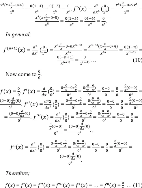
In general;

Q(_{ⁿ⁺¹⁾( ) =} ⁿ ⁿ( ⁿ) =

ⁿ∗T_U ∗ ⁽ⁿ⁻¹⁾

²ⁿ =

⁽ⁿ⁻¹⁾( ∗T_U ∗ )

²ⁿ =

( )

⁽ⁿ⁺¹⁾ =

( )

⁽ⁿ⁺¹⁾ = ⁽ⁿ⁺¹⁾ … (10)

Now come to .

Q( ) = . Q′( ) = ( ) = ∗

T U ∗TU

² = (_UT T_U)

² = = =

T

U( )

² = ( )_fUf( )

² . Q′′( ) = ^

²( ) = ∗_UT ∗T_U

² = (T_{U U}T)

² = = =

T

U( )

²

= ( )

f fU( )

² . Q′′′( ) = ³

³( ) = ∗T_U ∗T_U

² = (T_U T_U)

² = = =

T

U( )

² =

( )_fUf( ) ² ..

Qⁿ( ) = ⁿ_ⁿ( ) = ∗

T U ∗TU

² = (T_{U U}T)

² = = =

T

U( )

² = ( )_fUf( )

² .

Therefore;

Q( ) = Q′( ) = Q′′( ) = Q′′′( ) = Q⁴( ) = … = Qⁿ( ) = … (11) It is important to note that, in the above cases, it was dealt with normal derivatives and hence x was just a normal variable.

One should now consider x representing 0 i.e. letting x = 0.

Q( ) = = . Q′( ) = ( ) = ( ) = ∗ _² ∗ = ( _² ) =

( )

= . Q′′( ) = ²_²( ) = ∗

T

U ∗

² =

( )

² = ² = ^².Q′′′( ) = ³

³( ²) = ²∗T_U ∗

⁴ =

( ∗T_U ∗ )

⁴ = ³ = ³. Q⁴( ) = ⁴

⁴( ³) = ³∗T_U ∗ ^₂

⁶ =

²( ∗T_U ∗ )

⁶ = ⁴ = ⁴ . Q⁵( ) = ⁵

⁵( ⁴) = ⁴∗T_U ∗ ³

⁸ =

³( ∗_UT ∗ )

⁸ = ⁵ = ⁵. Replacing 0 with x, one gets:

Q′( ) = = = 1. Q′′( ) =

² = ² = . Q′′′( ) = ³ = ³ = ². Q⁴( ) =

⁴ = ⁴ = ³. Q⁵( ) = ⁵ = ⁵ = ⁴.

But at Q( ) = , it was proved that equation 11 is true, hence,

= = 1 = = _² = _³ = _⁴ = … Out of reasoning, it is only x = 1 that can satisfy the equation and therefore,

= 1 = = _² = _³ = _⁴ = … (12)

(viii)The method of limits (a)Approaching 0

This is a very robust method in proving that actually, = 1. It’s strong because, first, it’s used even in other problems and methods whenever there is a division or logarithms that are not direct and hence used whenever doubts arise. Secondly, it shows that limit does not approach 1, but, confirms that it’s actually 1. In this case, = and the solution obtained using the method of limits, does not approach 1 as one tends nearer and nearer to zero but it ascertains that whatever point one considers as very close to 0, one gets none other value but 1.

Since one has , then consider lim _→ $ ( . One should approach 0 from both left and right sides as in table 1.

Table 1. Limits from both sides of zero.

x → 0+ x 10-3 ₁₀-4 ₁₀-6 ₁₀-15 ₁₀-20 ₁₀-28 ₁₀-30

1 1 1 1 1 1 1

lim_→ $ ( 1 1 1 1 1 1 1

x → 0- x (-10)-3 _(-10)-4 _(-10)-6 _(-10)-15 _(-10)-20 _(-10)-28 _(-10)-30

1 1 1 1 1 1 1

lim_→ $ ( 1 1 1 1 1 1 1

Therefore, lim _→ $ ( = 1 and lim _→ $ ( = 1. Since there is no value closer to zero that gives any other solution other than 1, one can therefore conclude that this method does not approach 1 as one tends to 0 but the answer is 1(always).

(b)Using conjugates

Since one has lim _→ $ ( , the conjugate of x is x hence

lim → $ ( * $ ( = lim → $ ^_^ ( = lim → $ ( = limx->0 (1)= 1 … (13)

(c)Using L’Hospital’s Rule

Since one has lim _→ $ ( ,

then lim _→

fk fU fk

fU$ (

= limx->0 = limx->0 1 = 1… (14)

(ix) Method of introducing functions (Trigonometric functions)

lm

nop = ( ) = q. Given another one, = r, then pqr pqr = ( ) = r. This is true in any case of !_! = j, for all real numbers

y. For , let = y. Now introduce the cosine function to both

the numerator and denominator. Then it comes to nop_nop =( ) and one can also let x = 0 to have

( ) = nop_nop = nop_nop = … (15)

Therefore, nop_nop = = 1. Hence = y = 1, using the cosine function. Taking y to be 0 or ∞, would lead to confusion, i.e. = 0 would mean that = nop_nop = = 1 = y = 0 but it’s know

that 1 ≠ 0. Therefore, ≠ 0. Again, = ∞ would mean that = nop

nop = = 1 = y = ∞ but it’s known that 1 ≠ ∞. Therefore, ≠ ∞.

Now, introduce the tangent function to have = → str_str

= . Again, introduce the sine function to have = → pqr_pqr =

. But these two functions (sine and tangent) require us to use the method of limits, either approaching zero or the L’Hospital’s Rule.

Let us use the L’Hospital’s Rule.

limx->0 str

str = limx->0 = limx->0

fk

fUstr

fk

fUstr

= limx->0 punO

punO = lim

x->0 7 nop

v 8²

7 nopv 8²= 7 nop

v 8^

7 nopv 8^ = w v x²

y v z² = = 1. limx->0 pqr

pqr = limx->0 =

limx->0

fk fUpqr fk fUpqr

= limx->0 lm_lm = nop_lm = = = 1. Even if one uses

the method of limits and approaches 0 from both sides, it’s found that, at every point, the functions will always produce 1. That will also confirm that one is not tending to 1 but is at 1 always. This method is only applicable whenever the numerator and the denominator are equal such as and

does not apply if the two are different such as .

NB: An appeal is being made to anybody working out problems involving limits to use other methods to confirm the solution whenever direct substitution shows the results to be . That is; before concluding that = 1 as was seen in limits, other methods such as L’Hospital’s Rule should be employed because some situations are and can be deceptive. Some methods will confirm it while other cases will be shown otherwise.

(x) Method of self- operations

This method is also known as the method of Self- Addition, -Subtraction, -Multiplication and -Division.

In normal operations, whatever is done on the left hand side of an equation, the same is done on the right hand side of that equation. E.g. = m ⇒ * ( + 2) = m * ( + 2). Hence = 5 ⇒ * 3 = 5 * 3 i.e. 15 = 15. But in this method of self- arithmetic, whatever is done to the left hand side is different from what is done to the right hand side but still correct mathematically. E.g.

!² ! = k ⇒

!² ! +

!²

! = k + k… (16)

I.e. ; = 4 ⇒; + ; = 4 + 4. This is what is meant by self- operations:

I. If one subtracts the equation, then subtract the solution. II. If one adds the equation, then add the solution.

III.If one multiplies the equation by itself, then multiply the solution by itself.

IV.If one divides the equation by itself, then divide the solution by itself.

(a)Self- addition

For , let x = 0. Then = . Let the solution be y hence =

= y. By self- addition one gets + = y + y ⇒ ∗ _²∗ = 2y

⇒ ² ²_² = 2y ⇒ _²² = 2y ⇒ 2 = 2y ⇒ 1 = y hence y = 1. Therefore; = = y = 1. This is irrespective of whether one is to employ limits, L’Hospital’s Rule and cancellation rules or not.

(b)Self- subtraction

For , let x = 0. Then = . Let the solution be y hence =

= y. Then

- = y – y… (17)

Equation (17) ⇒ ∗ _² ∗ = y(1 – 1). Letting k = (1-1), then, ² ²

² = y(k) = yk ⇒ ²( )

² = yk ⇒ ({)

= yk ⇒ 1k = yk ⇒ 1 = y hence y =1. Therefore, = = y = 1.

Alternatively: - = y – y ⇒ = y(1 – 1) ⇒ ( ) = y(1 – 1) ⇒ ({) = y(k) ⇒ 1(k) = y(k) ⇒ 1 = y hence y = 1.

Therefore, = = y = 1. (c)Self- multiplication.

For , let x = 0. Then = . Let the solution be y hence = = y. By self- multiplication it becomes,

* = y*y… (18)

Equation (18) ⇒ ∗_∗ = y² →, ²_² = y² ⇒ 1 = y² ⇒ ±1 = ±y ⇒ 1 = y hence y = 1. Therefore, = = y = 1. NB: This was also seen in the method of powers.

(d)Self- division

For , let x = 0. Then = . Let the solution be y hence =

= y. By self- division one gets,

⁄ ⁄ =

!

! … (19)

Equation (19) ⇒ * = !_! or 1 ⇒ _²² = !_! or 1. = !_! or 1 ⇒ 1 = y hence y = 1. Therefore, = = y = 1.

(xi) The factorial method

procedure;

5

C5 = _{!( )!} ! = _{( )} = 1. This is similar for the case of x =

0 such that

0

C0 = _!( ! _)! = _{( )} = 1… (20)

For any equation = j, it’s allowed to deal with only the left hand side but whatever is done to the numerator, should also be done to the denominator. This gives one a chance to introduce factorials on both numerator and denominator. E.g. = y ⇒ !_! = = y where in both cases, y = 1. Therefore, = k ⇒ !_! = = k where in both cases, k = 1. This is not news for any non- negative numerator that is equal to its denominator i.e. For all whole numbers x, and !_! have the same

solutions. Examples are: = 1 and !_! = 1 ⇒ = !_! = = 1. = 1 and !_! = 1 ⇒ = !_! = = 1. = 1 and !_! = 1 ⇒ = !_! =

1. Therefore, = 1 and !_! = 1 ⇒ = !_! = = 1. If one says that k = 0 or k = ∞, then the results would be misleading. E.g. for k = 0, = k = 0 and hence !_! = 1 = k = 0 which would mean

that = 0 = !_! = 1 ⇒ 0 = 1 which is wrong. And for k = ∞, = k = ∞ and hence !_! = 1 = k = ∞ which would mean that = ∞

= !_! = 1 ⇒ ∞ = 1 which is also wrong. Prove that log $"_"( = 0.

Let x be 0 (x = 0). Then log $ ( = log $ (. Note that, the logarithm to base 10 is being used though any other base can be employed, it doesn’t change the results. Limits are used to have

log $ ( =lim _→ log $ ( . The method will approach 0 from both positive and negative sides (table 2).

Table 2. Logarithms from both sides of zero.

x → 0+ x 10-3 ₁₀-6 ₁₀-10 ₁₀-15 ₁₀-25 ₁₀-30 ₁₀-100

1 1 1 1 1 1 1

log$ ( 0 0 0 0 0 0 0

lim

→ €•‚ $ ( 0 0 0 0 0 0 0

x → 0- x (-10)-3 _(-10)-6 _(-10)-10 _(-10)-15 _(-10)-25 _(-10)-30 _(-10)-100

1 1 1 1 1 1 1

log$ ( 0 0 0 0 0 0 0

lim

→ €•‚ $ ( 0 0 0 0 0 0 0

One should know that it’s only log_{1 = 0 ∀ k „ (positive numbers). Therefore,

log $ ( = 0 = log 1… (21)

hence = 1.

Again, there’s no tending to 0 but confirming that the answer is 0.

(xii)The Logarithm base switch rule method

From the above proof, it’s also possible to prove that lim → log … = 0 i.e. x = ≠ 0 and lim

→N log … = 0 i.e. x = ≠ ∞ but lim

→†_/⁻log … = ∞ i.e. x = = 1 hence log_$TT( … = log … =

∞.

The logarithm base switch rule shows that,

log P = (log ‡)-1 = _ˆo‰

Š … (22)

E.g. log 5 = _ˆo‰

‹ = 0.69897004. log,10 = ˆo‰IT, =

2.302585093. Let b = 10 and c = , then it comes to,

log $ ( = _ˆo‰

$TT(

and since log $ ( = 0, then, 0 =

ˆo‰

$TT(

. Here, the question is, “What can one divide 1 with to

have 0?” I.e. “What is the value of y such that _! = 0?” In

normal circumstances, it is only the division of any real number by a very large number, say ∞, which can result in 0. I.e. _! = _N = 0. Therefore, the y must be a very large number,

say ∞. So, log_$T

T(10 = ∞. Let = k and hence log{10 = ∞.

One should be sure that, it’s only the logarithm to base 1 of any positive number that can give ∞, i.e. log 10 = ∞. This is true for all numbers. Therefore, log_{10 = log 10 = ∞ but k = hence log_{10 = log_$T

T(10 = log 10 = ∞. Therefore, one

can continue with equation whereby, 0 = _ˆo‰

$TT( ⇒

0 =

ˆo‰Œ = ˆo‰I = ˆo‰ $TT(

= _N = 0. In this method, the can

only be equal to 1 to have ∞ as the logarithm. Then, the ∞ divides 1 to bring it to 0 and hence both sides balance, 0 = 0. In general, = 1 using the logarithm base switch rule. NB: Even if one has 10 being replaced by 0, then it can result in

log 0 = - ∞ but _N = 0 also.

(xiii)The binomial expansion case method

Similarly, one has (• + ‡)3 = a3b0 + 3a2b1 + 3a1b2 + a0b3 = a3 + 3a2b + 3ab2 + b3. Now consider the following cases; (a)2 = a2 and (a)3 = a3.

And in general,

(a + b)n

= ∑ 7_‘’ r_‘8axbn-x = ∑_‘’r _{‘!(r ‘)!}r! axbn-x = r!t⁰_!r!“ⁿ +

r!t¹“ⁿ⁻¹ !(r )! +

r!t²“ⁿ⁻²

!(r )! + … + r!tⁿ“⁰

r! ! and (a)

n

= an. If one lets b = 0

in the case of (a + b)n, then it would result in; (a + 0)n =

r!t⁰ ⁿ !r! +

r!t¹ ⁿ⁻¹ !(r )! +

r!t² ⁿ⁻²

!(r )! + … + r!tⁿ ⁰

r! ! = 0 + 0 + 0 + … + r!tⁿ ⁰

r! ! = r!tⁿ ⁰

r! ! . But since r! r! ! =

n

Cn = 1, then (a + 0)n =

r!tⁿ ⁰ r! ! =

1 ∗ aⁿ ∗ 0⁰= an*00 = 00an. But it’s known that, (a + 0)n = (a)n = an, hence 00an = an ⇒ 00 = 1. Therefore, 00 = = 1. Simple cases are: (a + 0)2 = a200 + 2a101 + a002 but since 01 = 0, 02 = 0, a0 = 1, then (a + 0)2 = a200 + 0 +0 = a200 = 00a2. But (a + 0)2

= (a)2 = a2. This shows that, a2 = 00a2⇒ 00 = 1 and hence 00 = = 1. Again, (a + 0)3 = a300 + 3a201 + 3a102 + a003, but since 01 = 0, 02 = 0, 03 = 0, a0 = 1, then (a + 0)3 = a300 + 0 +0 + 0 = a300 = 00a3. But (a + 0)3 = (a)3 = a3. This shows that, a3 = 00a3⇒ 00 = 1 and hence

00 = = 1 … (23)

(xiv)The inverse- inverse method It is known that,

(X-1)-1 = X. Then,

(X-1) (X-1)-1 = 1... (24)

Let X = 2. Then (2-1)-1 = $ (-1 = $ ( = 2 ⇒ (X-1)-1 = X.

Again, (2-1)* (2-1)-1 = $ ( $ (-1 = (0.5) ($ (-1 = (0.5) (2) = 1 ⇒

(X-1) (X-1)-1 = 1. Also, if X = , then, ($ (-1 )-1 = (-4)-1 = ⇒ (X-1) (X-1)-1 = 1. But this can also be represented as: $ (-1 _{($ (}-1

)-1 = (-4) ($ (-1 )-1 = (-4) (-4)-1 = (-4) $ ( = (-4) (-0.25) = 1 ⇒ (X-1) (X-1)-1 = 1. Consider the part involving X = 2. Then, (2-1)-1 = $ (-1 = (0.5)-1 = _. = 2. Again, (2-1)* (2

-1

)-1 = $ ( $ (-1 = (0.5) $ (-1 = (0.5)(2) = 1. Hence (2-1)*(2-1)-1

= $ ( $ (-1 = $ ( (2) = = 1. In the next case, let y= 0. Then,

(y-1) (y-1)-1 = $_!( $_!(-1 = $_!($!( = $!_!( = 1, because (X-1) (X

-1

)-1 = 1. Alternatively, let again y = 0. For , one has !_!. Then, $!_!(-1 _($!

!(

-1

)-1 = $!_!($!_!(-1 = $!_!($!_!( = $!²_!²( = 1 ⇒$ ( = $ ²_²( = 1.

Testing other solutions

Let = x. 1st case, let = x = 0. 2nd case, let = x = 1. 3rd

case, let = x = ∞.

1st case, = x = 0. Then, (0-1) (0-1)-1 = $ ($ (-1 = (∞) $ (-1

= (∞)$ (= ∞*0 = 0 (shown using limits). But 0 ≠ 1 hence

does not fulfil the condition of (X-1) (X-1)-1 = 1. 2nd case, = x

= 1. Then, (1-1) (1-1)-1 = $ ($ (-1 = (1) $ (-1 = (1) $ ( = (1)

(1) = 1*1 = 1. But 1 = 1, hence fulfils the condition of (X-1) (X-1)-1 = 1. 3rd case, = x = ∞. Then, (∞-1) (∞-1)-1 = $_N($_N(-1

= (0) $_N(-1 = (0) $N( = 0*∞ = 0 (shown using limits). But 0 ≠ 1 hence does not fulfil the condition of (X-1) (X-1)-1 = 1. Conclusion: It’s only 2nd case, = x = 1, that satisfies the condition of (X-1) (X-1)-1 = 1. Therefore it can be conclude that = 1.

NB: Limits have been used (method of approaching from both sides) to show that _N ⇒ 0, → ∞, ∞*0 ⇒ 0 and 0*∞ ⇒ 0. It’s also good to note that, using the limits method, → +∞ or → −∞ but in both cases, 0*∞ and ∞*0 tend to 0 irrespective of whether the ∞ is positive or negative.

(xv)The method of geometric series (G.P)

Let the geometric series knowledge be used to see what

is. The three cases of = x when x = 1, x = 0, x = ∞ will be tested hence the idea of limits will help argue the cases out. In a geometric series, when r = 1, then Sn = na and a1 = a2 =

a3 = … = an = … = a∞. If r = 1, then the series, though

geometric, is also an arithmetic series (A.P) with d = 0 and a1

= a2 = a3 = … = an = … = a∞. In this case of A.P,

Sn = n [2a + (n – 1)d] = n (2a) = n (a + l) … (25)

where l is the last term of the series.

Example 1: 2 + 2 + 2 + 2 + 2. For G.P case, r = = 1, a = a1 = a2 = a3 = a4 = a5 = 2, n = 5. Sn = na ⇒ S5 = 5(2) = 10. For

A.P case, d = 2 – 2 = 0, a = a1 = a2 = a3 = a4 = a5 = 2, n = 5, l

= 2. Sn = n (2a) ⇒ S5 = (2*2) = (4) = 5(2) = 10. Or Sn =

n (a + l) ⇒ S5 = (2+2) = 5(2) = 10. Therefore, S5 = 10 for

both G.P and A.P, when r = 1 or d = 0 respectively.

Example 2: 1 + 1 + 1 + 1 + 1 + 1 + 1 + 1. For G.P case, r = = 1, a = a1 = a2 = a3 = … = a8 = 1, n = 8. Sn = na ⇒ S8 =

8(1) = 8. For A.P case, d = 1 – 1 = 0, a = a1 = a2 = a3 = … =

a8 = 1, n = 8, l = 1. Sn = n (2a) ⇒ S8 =

;

(2*1) = ; (2) = 8(1). Or Sn = n (a + l) ⇒ S8 = ; (1+1) = ; (2) = 8(1). Therefore, S8

= 8 for both G.P and A.P, when r = 1 or d = 0 respectively. NB: The above scenarios hold for all cases, where r = 1 or d = 0.

Now let the concentrate be on the G.P part. It’s known that if r = 1, then Sn = a1 + a2+ a3 + … + an⇒ a1 = a2 = a3 = … =

an. Let the number of terms be reduced to 5 only. Then, a1 +

a2+ a3 + a4 + a5 is the new G.P. If r = 1, then a1 = a2 = a3 = a4 =

a5. But r =

tӠI

t” hence r =

tO

tI =

t•

tO =

t–

t•=

t‹

t–= 1. Now, focus on the series below up to 5th term; + + + + , n = 5. Let it

be replaced by x1 + x2 + x3 + x4 + x5 where xi = and hence,

x1 = x2 = x3 = x4 = x5 and r =

7 v 8

7 v 8 = * =

1st Case, r = = 0. Here, it’s meant that ‘_‘O

I = 0, • O = 0,

– • =

0, ‹

– = 0.

But from limits, it’s possible to have this scenario iff the numerator is any real number, rn, and the denominator is a very large number, say ∞. Then one would have;

‘O

‘I =

—

N = 0 … (26)

• O =

—

N = 0 … (27)

– • =

—

N = 0 ... (28)

‹ – =

—

N = 0 … (29)

Consider (26) and (27). In (26), x2 = rn (any real number)

but in (27), the x2 = ∞. But it’s true that in both cases, x2(26) =

x2(27). Then it would mean that x2(26) = x2(27) = rn = ∞. This is a

contradiction because any real number, rn, is not equal to ∞. Therefore, rn ≠ ∞. Hence this fails to hold true when it’s taken that r = = 0. Therefore, r = ≠ 0. If one decides to compare the other x’s, the same results will be found, meaning that;

(x2 = rn)(26) ≠ (x2 = ∞)(27), (x3 = rn)(27) ≠ (x3 = ∞)(28), (x4 =

rn)(28) ≠ (x4 = ∞)(29) and in general,

(xi = rn)≠ (xi = ∞) which implies that, r ≠ 0 hence ≠ 0.

E.g. 5 ≠ ∞, -2 ≠ ∞, ≠ ∞, 500 ≠ ∞, etc.

2nd Case, r = = 1. Here, it’s meant that ‘_‘O

I = 1, • O = 1,

– • =

1, ‹

– = 1. Whether from limits or normal operations of

numbers, this scenario is only possible iff the numerator is equal to the denominator. And can be any real number, say -10, -1/3, 2, 4, 5.7, etc. In these cases, there is no contradiction. Take for example both the numerator and denominator to be 5. Then

‘O

‘I = = 1 … (30)

•

O = = 1 … (31)

–

• = = 1 … (32)

‹

– = = 1 … (33)

Consider (30) and (31) in this case. In (30), x = 5 and in (31), x = 5. Compare all the x’s in all the equations above. It

will, for example, be found that x2(30) = x2(31) = 5, meaning

that there is no contradiction. Whatever number one may take to be the numerator as well as the denominator, no contradiction will arise. This shows that for r = 1, hence =

1, there is no contradiction at all. Therefore, r = = 1.

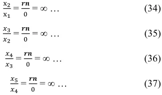
3rd Case, r = = ∞. Here, it’s meant that, ‘_‘O

I = ∞, • O = ∞,

– •

= ∞, ‹

– = ∞. From limits, this scenario is possible iff the

numerator is any real number, rn, and the denominator is a very small number, say 0. That is to say;

‘O

‘I =

™š

= ∞ … (34)

• O =

™š

= ∞ … (35)

– • =

™š

= ∞ … (36)

‹ – =

™š

= ∞ … (37)

Consider the equations (34) and (35) above. In (34), x2 =

rn (any real number), but in (35), x2 = 0. But it’s true that

x2(34) = x2(35). Then, it would imply that x2(34) = x2(35) = rn = 0.

Since this is a contradiction, then;

(x2 = rn)(34) ≠ (x2 = 0)(35), (x3 = rn)(35) ≠ (x3 = 0)(36), (x4 =

rn)(36) ≠ (x4 = 0)(37). And in general,

(xi = rn)≠ (xi = 0) which implies that, r = ≠ ∞. E.g. 5 ≠ 0,

-2 ≠ 0, -1/5 ≠ 0, 500 ≠ 0, etc.

Conclusion: In general, r = ≠ 0 and r = ≠ ∞ because

they bring contradiction. But r = = 1 has no contradiction in the geometric series method with r = 1.

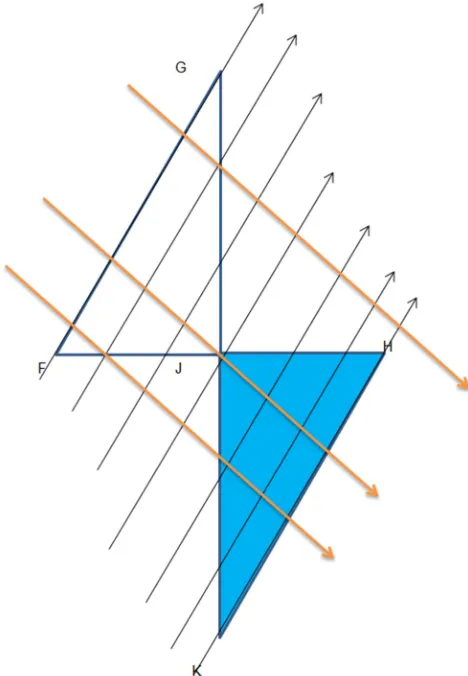
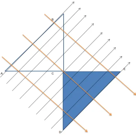
(xvi)Zero as an interval, a range and a point

An interval, say [y1, y2], can be converted into a range and

consequently, it can be minimized to a point. This is the whole idea in any given point. Consider any interval, [y1, y2]

that can be converted into a range y1 - y2 for y2 – y1 (Figure

1). But even if y1 > y2, the operation would bear the same

results. Take real numbers for y1 and y2, say y1 = 4, y2 = 10.

Then one would have [y1, y2] = [4, 10] and the range would

be y2 - y1 = 10 – 4 = 6 units. In all cases of real numbers, 0

can be represented as an interval and a range as well. In such a case, one only needs to reduce the interval until y1 = y2 and

this would bring the results to 0, i.e. y2 - y1 = 0 because y2

would be equal to y1 (y2 = y1 hence y2 - y1 = 0). This can be

achieved in several ways. One way is to fix y1 and moving y2

closer and closer to y1 until y2 becomes y1 (Figure 4). When

the two are equal, then at that, there’s a point and not a range. This point is zero, i.e. has a range 0 (y1 – y2 = 0). The second

way is to fix y2 and moving y1 closer and closer to y2 until y1

becomes y2 (Figure 2). When the two are equal, then at that,

there’s a point and not a range. This point is zero, i.e. has a range 0 (y2 - y1 = 0). The last way to achieve the same results

is to consider both y1 and y2 simultaneously. Instead of fixing

any point, one may decide to move both towards each other until the two meet at a new point (Figure 3). One moves the two at an equal rate and when they meet, y1 = y2 and hence y2

- y1 = 0 or y1 – y2 = 0. The whole thing becomes a point

eventually. One can see the illustrations below:

Figure 1. Original interval.

Figure 3. Varying y1 and y2 simultaneously.

Figure 4. Fixing y1.

Mathematically, let y1 = 4 and y2 = 10. Then y2 - y1 = 10- 4

= 6. Reduce y2 by 3 units, then one has y21 = 7. Here, y21 - y1

= 7- 4 = 3. Reduce y21 by 2, then one has y22 = 5. Here, y22 -

y1 = 5- 4 = 1. Reduce y22 by 0.5, then one has y23 = 4.5. Here,

y23 - y1 = 4.5- 4 = 0.5. Reduce y23 by 0.09, then one has y24 =

4.41. Here, y24 - y1 = 4.41- 4 = 0.41. Reduce y2i until y2i› y1,

i.e. y2i - y1 › 0. In this case, one had fixed y1. If one fixes y2

in the next case, it will involve increasing y1 by some length

until y1i› y2, i.e. y1i - y2 › 0. In practical; y2 - y1 = 10- 4 = 6.

Increase y1 by 3 units, then one has y11 = 7. Here, y2 - y11 =

10- 7 = 3. Increase y11 by 2, then one has y12 = 9. Here, y2 -

y12 = 10- 9 = 1. Increase y12 by 0.5, then one has y13 = 9.5.

Here, y2 - y13 = 10- 9.5 = 0.5. Increase y13 by 0.09, then one

has y14 = 9.59. Here, y2 - y14 = 10- 9.59 = 0.41. Continue to

increase y1i until y1i› y2, i.e. y2 - y1i › 0.

The last case involves changing both y1 and y2. Here, even

if one does not vary y1 and y2 by equal lengths, what is finally

proved is the same. Let y1 = 2 and y2 = 10. Then, y2 – y1 = 10 – 2 = 8. Reduce y2 by 2 and increase y1 by 2. Then, one has y2 = 8, y1 = 4 and y2 – y1 = 8 – 4 = 4. Increase y1 by 1 and reduce y2 by 1 to get y1 = 5, y2 = 7 and y2 – y1 = 7 – 5 = 2. Increase y1 by 0.8 and reduce y2 by 0.8 to get y1 = 5.8, y2 = 6.2 and y2 – y1 = 6.2 – 5.8 = 0.4. Increase y1 by 0.18 and reduce y2 by 0.18 to get y1 = 5.98, y2 = 6.02 and y2 – y1

= 6.02 – 5.98 = 0.04. One can continue with this process until y1› y2 and hence y2 - y1 › 0.These three cases illustrate how

it is possible turn a range into a point, say a big interval into a small interval of, say length 0.Suppose that at each stage of the three cases, one was performing reduction and this was followed by division of the resulting interval in terms of a range. I.e. !ₐₑ !ₓₔ_{!ₐₑ !ₓₔ}. For case 1 and case 2, it would have been

= = 1, F_F = = 1, = = 1, . _. = . _. = 1, ._. = .

. = 1 etc. And for case 3, it would have been

= ;_; = 1, ;_; = = 1, F _F = = 1, . .;_{. .;} = ._. = 1, . . ;

. . ; = .

. = 1 etc.

Note that, no matter how small one tries to make the range or interval, the division of what remains in order to get 0 (point) is always 1. This proves that one needs to see that 0 is an interval as well as a range reduced to a point. Therefore, since 0 = range/ interval, then it can be concluded that

= — ,_{— ,} = ¡ -,—¢ £_{¡ -,—¢ £} = 1… (38)

This can also be seen in the uniform distribution whose probability distribution function (pdf) is proved to be a pdf by dividing a range/ interval by itself. NB: The division of a range/interval in the above results can also be used to prove the gradient of a point as 1.

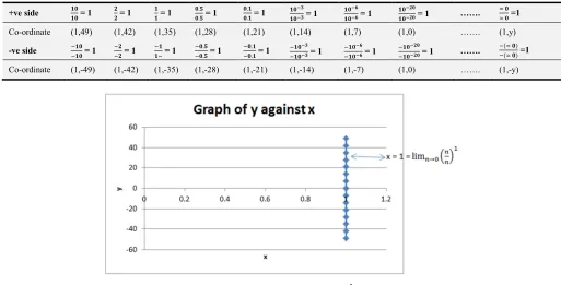
(xvii)The graphical method

One may want to try and see where the graph of x = cuts the x-axis. In this method, zero is being approached from both sides. Note that one can also use the graph of y = and see

where it cuts the y-axis. Therefore, let x = . From the positive and negative sides, then approach 0 as shown in table 3.

Table 3. Co-ordinates for graphing.

+ve side ¤"

¤" = 1 ¥ ¥ = 1

¤ ¤ = 1

".¦ ".¦ = 1

".¤

".¤ = 1 ¤" H§

¤"H§ = 1 ¤" H¨

¤"H¨ = 1 ¤" H¥"

¤"H¥" = 1 …….

≃ " ≃ " =1

Co-ordinate (1,49) (1,42) (1,35) (1,28) (1,21) (1,14) (1,7) (1,0) ……. (1,y)

-ve side ¤"

¤" = 1 ¥ ¥ = 1

¤ ¤ = 1

".¦ ".¦ = 1

".¤ ".¤ = 1

¤"H§ ¤"H§ = 1

¤"H¨ ¤"H¨ = 1

¤"H¥"

¤"H¥" = 1 ……. (≃ ") (≃ ") =1

Co-ordinate (1,-49) (1,-42) (1,-35) (1,-28) (1,-21) (1,-14) (1,-7) (1,0) ……. (1,-y)