Regularization on Graphs with Function-adapted Diffusion Processes
Arthur D. Szlam [email protected]
Department of Mathematics U.C.L.A., Box 951555 Los Angeles, CA 90095-1555
Mauro Maggioni [email protected]
Department of Mathematics and Computer Science Duke University, Box 90320
Durham, NC, 27708
Ronald R. Coifman [email protected]
Program in Applied Mathematics Department of Mathematics Yale University, Box 208283 New Haven,CT,06510
Editor: Zoubin Ghahrmani
Abstract
Harmonic analysis and diffusion on discrete data has been shown to lead to state-of-the-art algo-rithms for machine learning tasks, especially in the context of semi-supervised and transductive learning. The success of these algorithms rests on the assumption that the function(s) to be studied (learned, interpolated, etc.) are smooth with respect to the geometry of the data. In this paper we present a method for modifying the given geometry so the function(s) to be studied are smoother with respect to the modified geometry, and thus more amenable to treatment using harmonic analy-sis methods. Among the many possible applications, we consider the problems of image denoising and transductive classification. In both settings, our approach improves on standard diffusion based methods.
Keywords: diffusion processes, diffusion geometry, spectral graph theory, image denoising,
trans-ductive learning, semi-supervised learning
1. Introduction
sparsity in a “Fourier” basis, and evolution of heat that are well-known in Euclidean spaces (Zhou and Schlkopf, 2005).
One of the main contributions of this work is the observation that the geometry of the space is not the only important factor to be considered, but that the geometry and the properties of the function
f to be studied (denoised/learned) should also affect the smoothing operation of the diffusion. We
will therefore modify the geometry of a data set with features from f , and build K on the modified
f -adapted data set. The reason for doing this is that perhaps f is not smooth with respect to the
geometry of the space, but has structure that is well encoded in the features. Since the harmonic analysis tools we use are robust to complicated geometries, but are most useful on smooth functions, it is reasonable to let the geometry of the data set borrow some of the complexity of the function, and study a smoother function on a more irregular data set. In other words, we attempt to find the geometry so that the functions to be studied are as smooth as possible with respect to that geometry. On the one hand, the result is nonlinear in the sense that it depends on the input function f , in contrast with methods which consider the geometry of the data alone, independently of f . On the other hand, on the modified data set, the smoothing operator K will be linear, and very efficiently computable. One could generalize the constructions proposed to various types of processes (e.g., nonlinear diffusions).
The paper is organized as follows: in Section 2, we review the basic ideas of harmonic analysis on weighted graphs. In Section 3 we introduce the function-adapted diffusion approach, which aims to modify the geometry of a data set so that a function or class of functions which was non-smooth in the original geometry is smooth in the modified geometry, and thus amenable to the harmonic analysis in the new geometry. In Section 4 we demonstrate this approach in the context of the image denoising problem. In addition to giving easy to visualize examples of how the method works, we achieve state of the art results. In Section 5, we demonstrate the approach in the context of transductive learning. While here it is more difficult to interpret our method visually, we test it on a standard database, where it outperforms comparable “geometry only” methods on the majority of the data sets, and in many cases achieves state of the art results. We conclude by considering the under-performance of the method on some data sets, observing that in those examples (most of which are in fact the only artificial ones!), the geometry of the data suffices for learning the function of interests; and our method is superfluous.
2. Diffusion on Graphs Associated with Data-sets
An intrinsic analysis of a data set, modeled as a graph or a manifold, can be developed by consid-ering a natural random walk K on it (Chung, 1997; Szummer and Jaakkola, 2001; Ng et al., 2001; Belkin and Niyogi, 2001; Zha et al., 2001; Lafon, 2004; Coifman et al., 2005a,b). The random walk allows to construct diffusion operators on the data set, as well as associated basis functions. For an initial conditionδx, Ktδx(y)represents the probability of being at y at time t, conditioned on starting
at x.
2.1 Setup and Notation
We consider the following general situation: the space is a finite weighted graph G= (V,E,W), consisting of a set V (vertices), a subset E (edges) of V×V , and a nonnegative function W : E→R+
the edges will be undirected. The techniques we propose however do not require this property, and therefore can be used on data sets in which graph models with directed edges are natural.
We interpret the weight W(x,y)as a measure of similarity between the vertices x and y. A natural filter acting on functions on V can be defined by normalization of the weight matrix as follows: let
d(x) =
∑
y∈V
W(x,y),
and let1the filter be
K(x,y) =d−1(x)W(x,y), (1) so that∑y∈VK(x,y) =1, and so that multiplication K f of a vector from the left is a local averaging operation, with locality measured by the similarities W . Multiplication by K can also be interpreted as a generalization of Parzen window type estimators to functions on graphs/manifolds. There are other ways of defining averaging operators. For example one could consider the heat kernel
e−tL where
L
is defined in (3) below, see also Chung (1997), or a bi-Markov matrix similar to W (Sinkhorn, 1964; Sinkhorn and Knopp, 1967; Soules, 1991; Linial et al., 1998; Shashua et al., 2005; Zass and Shashua, 2005).In general K is not column-stochastic,2but the operation f K of multiplication on the right by a (row) vector can be thought of as a diffusion of the vector f . This filter can be iterated several times by considering the power Kt.
2.2 Graphs Associated with Data Sets
¿From a data set X we construct a graph G: the vertices of G are the data points in X , and weighted edges are constructed that connect nearby data points, with a weight that measures the similarity between data points. The first step is therefore defining these local similarities. This is a step which is data- and application-dependent. It is important to stress the attribute local. Similarities between far away data points are not required, and deemed unreliable, since they would not take into account the geometric structure of the data set. Local similarities are assumed to be more reliable, and non-local similarities will be inferred from local similarities through diffusion processes on the graph.
2.2.1 LOCALSIMILARITIES
Local similarities are collected in a matrix W , whose rows and columns are indexed by X , and whose entry W(x,y)is the similarity between x and y. In the examples we consider here, W will usually be symmetric, that is the edges will be undirected, but these assumptions are not necessary.
If the data set lies inRd, or in any other metric space with metricρ, then the most standard construction is to choose a number (“local time”)σ>0 and let
Wσ(x,y) =h ρ
(x,y)2 σ
,
1. Note that d(x) =0 if and only if x is not connected to any other vertex, in which case we trivially define d−1(x) =0, or simply remove x from the graph.
for some function h with, say, exponential decay at infinity. A common choice is h(a) =exp(−a). The idea is that we expect that very close data points (with respect toρ) will be similar, but do not want to assume that far away data points are necessarily different.
Let D be the diagonal matrix with entries given by d as in (2.1). Suppose the data set is, or lies on, a manifold in Euclidean space. In Lafon (2004), Belkin and Niyogi (2005), Hein et al. (2005), von Luxburg et al. (2004) and Singer (2006), it is proved that in this case, the choice of h in the construction of the weight matrix is in some asymptotic sense irrelevant. For a rather generic
symmetric function h, say with exponential decay at infinity,(I−D− 1 2
σ WσD− 1 2
σ )/σ, approaches the Laplacian on the manifold, at least in a weak sense, as the number of points goes to infinity andσ goes to zero. Thus this choice of weights is naturally related to the heat equation on the manifold. On the other hand, for many data sets, which either are far from asymptopia or simply do not lie on a manifold, the choice of weights can make a large difference and is not always easy. Even if we use Gaussian weights, the choice of the “local time parameter”σcan be nontrivial.
For each x, one usually limits the maximum number of points y such that W(x,y) 6=0 (or non-negligible). Two common modifications of the construction above are to use either ρε(x,y)
orρk(x,y)instead ofρ, where
ρε(x,y) =
d(x,y) ifρ(x,y)≤ε;
∞ ifρ(x,y)>ε ,
where usuallyεis such that h(ε2/σ)<<1, and ρk(x,y) =
ρ
(x,y) if y∈nk(x);
∞ otherwise.
and nk(x)is the set of k nearest neighbors of x. This is for two reasons: one, often only very small
distances give information about the data points, and two, it is usually only possible to work with very sparse matrices.3 This truncation causes W to be not symmetric; if symmetry is desired, W may be averaged (arithmetically or geometrically) with its transpose.
A location-dependent approach for selecting the similarity measure is suggested in Zelnik-Manor and Perona (2004). A number m is fixed, and the distances at each point are scaled so the m-th nearest neighbor has distance 1; that is, we letρx(y,y0) =ρ(y,y0)/ρ(x,xm), where xmis the m-th nearest neighbor to x. Nowρxdepends on x, so in order to make the weight matrix symmetric,
they suggest to use the geometric mean ofρxandρyin the argument of the exponential, that is, let
Wσ(x,y) =h ρ
x(x,y)ρy(x,y) σ
, (2)
with h, as above, decaying at infinity (typically, h(a) =exp(−a)), or truncated at the k-th nearest neighbor. This is called the self-tuning weight matrix. There is still a timescale in the weights, but a globalσ in the self-tuning weights corresponds to some location dependent choice ofσ in the standard exponential weights.
2.2.2 THEAVERAGINGOPERATOR ANDITSPOWERS
Multiplication by the normalized matrix K as in (1) can be iterated to generate a Markov process
{Kt}
t≥0, and can be used to measure the strength of all the paths between two data points, or the
likelihood of getting from one data point to the other if we constrain ourselves to only stepping between very similar data points. For example one defines the diffusion or spectral distance (B ´erard et al., 1994; Coifman et al., 2005a; Coifman and Lafon, 2006a) by
D
(t)(x,y) =||Kt(x,·)−Kt(y,·)|| 2=r
∑
z∈X
|Kt(x,z)−Kt(y,z)|2.
The term diffusion distance was introduced in Lafon (2004), Coifman et al. (2005a) and Coifman and Lafon (2006a) and is suggested by the formula above, which expresses
D
(t)as some similarity between the probability distributions Kt(x,·)and Kt(y,·), which are obtained by diffusion from x and y according to the diffusion process K. The term spectral distance was introduced in B ´erard et al. (1994, see also references therein). It has recently inspired several algorithms in clustering, classification and learning (Belkin and Niyogi, 2003a, 2004; Lafon, 2004; Coifman et al., 2005a; Coifman and Lafon, 2006a; Mahadevan and Maggioni, 2005; Lafon and Lee, to appear, 2006; Mag-gioni and Mhaskar, 2007).2.3 Harmonic Analysis
The eigenfunctions{ψi}of K, satisfying
Kψi=λiψi,
are are related,via multiplication by D−12, to the eigenfunctionsφi of the graph Laplacian (Chung,
1997), since
L
=D−12W D−1
2 −I=D 1 2KD−
1
2 −I. (3)
They lead to a natural generalization of the Fourier analysis: any function g∈L2(X)can be written as g=∑i∈Ihg,φiiφi, since{φi} is an orthonormal basis. The larger is i, the more oscillating the
functionφiis, with respect to the geometry given by W , andλimeasures the frequency ofφi. These
eigenfunctions can be used for dimensionality reduction tasks (Lafon, 2004; Belkin and Niyogi, 2003a; Coifman and Lafon, 2006a; Coifman et al., 2005a; Jones et al., 2007a,b).
For a function g on G, define its gradient (Chung, 1997; Zhou and Schlkopf, 2005) as the function on the edges of G defined by
∇g(x,y) =W(x,y) pg(y) d(y)−
g(x)
p d(x)
!
(4)
if there is an edge e connecting x to y and 0 otherwise; then
||∇g(x)||2=
∑
x∼y
|∇g(x,y)|2.
The smoothness of g can be measured by the Sobolev norm
||g||2H1=
∑
x
|g(x)|2+
∑
x
The first term in this norm measures the size of the function g, and the second term measures the size of the gradient. The smaller||g||H1, the smoother is g. Just as in the Euclidean case,
||g||2H1 =||g|2L2(X,d)− hg,
L
gi;thus projecting a function onto the first few terms of its expansion in the eigenfunctions of
L
is a smoothing operation.4We see that the relationships between smoothness and frequency forming the core ideas of Eu-clidean harmonic analysis are remarkably resilient, persisting in very general geometries. These ideas have been applied to a wide range of tasks in the design of computer networks, in paral-lel computation, clustering (Ng et al., 2001; Belkin and Niyogi, 2001; Zelnik-Manor and Perona, 2004; Kannan et al., 2004; Coifman and Maggioni, 2007), manifold learning (B ´erard et al., 1994; Belkin and Niyogi, 2001; Lafon, 2004; Coifman et al., 2005a; Coifman and Lafon, 2006a), image segmentation (Shi and Malik, 2000), classification (Coifman and Maggioni, 2007), regression and function approximation (Belkin and Niyogi, 2004; Mahadevan and Maggioni, 2005; Mahadevan et al., 2006; Mahadevan and Maggioni, 2007; Coifman and Maggioni, 2007).
2.4 Regularization by Diffusion
It is often useful to find the smoothest function ˜f on a data set X with geometry given by W , so
that for a given f , ˜f is not too far from f ; this task is encountered in problems of denoising and
function extension. In the denoising problem, we are given a function f+ηfrom X →R, andη is Gaussian white noise of a given variance, or if one is ambitious, some other possibly stochastic contamination. We must find f . In the function extension or interpolation problem, a relatively large data set is given, but the values of f are known at only relatively few “labeled” points, and the task is to find f on the “unlabeled” points. Both tasks, without any a priori information on f , are impossible; the problems are underdetermined. On the other hand, it is often reasonable to assume
f should be smooth, and so we are led to the problem of finding a smooth ˜f close to f .
In Euclidean space, a classical method of mollification is to run the heat equation for a short time with initial condition specified by f . It turns out that the heat equation makes perfect sense on a weighted graph: if f is a function on V , set f0= f , and fk+1=K f . If gk(x) =d
1
2(x)fk(x),
gk+1−gk=
L
gk,so multiplication by K is a step in the evolution of the (density normalized) heat equation. Further-more, a quick calculation shows this is the gradient descent for the smoothness energy functional
∑||∇g||2. We can thus do “harmonic” interpolation on X by iterating K (Zhu et al., 2003).
We can design more general mollifiers using an expansion on the eigenfunctions {ψi} of K.
For the rest of this section, suppose all inner products are taken against the measure d, that is,
ha,bi=∑a(x)b(x)d(x), and so ψare orthonormal. Then f =∑hf,ψiiψi and one can define ˜f , a
smoothed version of f , by
˜
f=
∑
i
αihf,ψiiψi
for some sequence{αi}which tends to 0 as i→+∞; in the interpolation problem, we can attempt
to estimate the inner productshf,ψii, perhaps by least squares. Typical examples forαiare:
(i) αi=1 if i<I, and 0 otherwise (pure low-pass filter); I usually depends on a priori information
onη, for example on the variance ofη. This is a band-limited projection (with band I), see for example Belkin (2003).
(ii) αi=λtifor some t>0, this corresponds to setting ˜f=Kt(f), that is, kernel smoothing on the
data set, with a data-dependent kernel (Smola and Kondor, 2003; Zhou and Schlkopf, 2005; Chapelle et al., 2006).
(iii) αi=P(λi), for some polynomial (or rational function) P, generalizing (ii). See, for example,
Maggioni and Mhaskar (2007)
As mentioned, one can interpret Ktf as evolving a heat equation on the graph with an initial
condi-tion specified by f . If we would like to balance smoothing by K with fidelity to the original f , we can chooseβ>0 and set f0= f and ft+1= (K ft+βf)/(1+β); the original function is treated as
a heat source. This corresponds at equilibrium to
(iv) αi=β/(1+β−λi).
One can also consider families of nonlinear mollifiers, of the form
˜
f=
∑
i
m(hf,ψii)ψi,
where for example m is a (soft-)thresholding function (Donoho and Johnstone, 1994). In fact, m may be made even dependent on i. While these techniques are classical and well-understood in Euclidean space (mostly in view of applications to signal processing), it is only recently that research in their application to the analysis of functions on data sets has begun (in view of applications to learning tasks, see in particular Maggioni and Mhaskar 2007).
All of these techniques clearly have a regularization effect. This can be easily measured in terms of the Sobolev norm defined in (5): the methods above correspond to removing or damping the components of f (or f+η) in the subspace spanned by high-frequencyψi, which are the ones
with larger Sobolev norm.
3. Function-adapted Kernels
points where f has similar structure, in addition to being near to each other in terms of the given geometry of the data.
The simplest version of this idea is to only choose nonzero weights between points on the same level set of f . Then||∇f||(with respect to W ) is zero everywhere, and the function to be recovered is as smooth as possible. Of course knowing the level sets of f is far too much to ask for in practice. For example, in the function extension problem, if f has only a few values (e.g., for a classification task), knowing the level sets of f would be equivalent to solving the problem.
If we had some estimate ˜f for f , we could set
Wf(x,y) =exp
−||x−y|| 2
σ1 −
|f˜(x)−f˜(y)|2 σ2
, (6)
so that whenσ2<<σ1, the associated averaging kernel K will average locally, but much more along the (estimated) level sets of f than across them, because points on different level sets now have very weak or no affinity. This is related to ideas in Yaroslavsky (1985); Smith and Brady (1995) and Coifman et al. (2005a).
The estimate ˜f of f is just a simple example of a feature map. More generally, we set
Wf(x,y) =h1
−ρ1(x,y) 2 σ1
h2
−ρ2(
F
(f)(x),F
(f)(y)) 2 σ2
, (7)
where
F
(f)(x) is a set of features associated with f , evaluated at the data point x,ρ1 is a metric on the data set,ρ2is a metric on the set of features, h1and h2are (usually exponentially) decayingfunctions, andσ1andσ2are “local time” parameters in data and feature space respectively. Such a similarity is usually further restricted as described at the end of Section 2.2.1. The idea here is to be less ambitious than (6), and posit affinity between points where we strongly believe f to have the same structure, and not necessarily between every point on an (estimated) level set. The averaging matrix Kf associated with Wf can then be used for regularizing, denoising and learning tasks, as described above. We call such a kernel a function-adapted kernel.
The way the function f affects the construction of Kf will be application- and data- specific, as we shall see in the applications to image denoising and graph transductive learning. For example, in the application to image denoising,
F
(f)(x)may be a vector of filter responses applied to the imagef at location x. In the application to transductive classification, we are given C functionsχi, defined
byχi(x) =1 if x is labeled as a point in class i, and 0 otherwise (either the point is not labeled, or it
is not in class i). We set f = (χi)Ni=1. Then
F
(f)(x)can be obtained by evaluating Kt(χi)at x, where K is a diffusion operator which only depends on the data set, and not on theχi’s. In all applications,our idea is simply to to try to choose similarities, with the limited information about the function(s) to be recovered that we are given, so that the function(s) are as regular as possible with respect to the chosen similarities.
4. Application I: Denoising of Images
We apply function-adapted kernels to the task of denoising images. Not only this will be helpful to gain intuition about the ideas in Section 3 in a setting where our methods are easily visualized, but it also leads to state-of-art results.
Gray-scale images are often modeled as real-valued functions, or distributions, on Q, a fine discretization of the square[0,1]2, and they are often analyzed, denoised, compressed, inpainted,
Chan and Shen (2005), Perona and Malik (1990), Tomasi and Manduchi (1998), Elad (2002), Boult et al. (1993), Chin and Yeh (1983), Davis and Rosenfeld (1978), Graham (1961), Huang et al. (1979), Lee (1980), Yin et al. (1996) and references therein. It is well known that images are not smooth as functions from Q toR, and in fact the interesting and most important features are often exactly the non-smooth parts of f . Thus Fourier analysis and the heat equation on Q are not ideally suited for images; much of the work referenced above aims to find partial differential equations whose evolution smooths images without blurring edges and textures.
With the approach described in Section 3, unlike with many PDE-based image processing meth-ods, the machinery of smoothing is divorced from the task of feature extraction. We build a graph
G(I)whose vertices are the pixels of the image and whose weights are adapted to the image struc-ture, and use the diffusion on the graph with a fidelity term, as described in Section 2.4 to smooth the image, considered as a function on the graph. If we are able to encode image structure in the geometry of the graph in such a way that the image is actually smooth as a function on its graph, then the harmonic analysis on the graph will be well-suited for denoising that image. Of course, we have shifted part of the problem to feature extraction, but we will see that very simple and intuitive techniques produce state of the art results.
4.1 Image-adapted Graphs and Diffusion Kernels
To build the image-adapted graph we first associate a feature vector to each location x in the image
I, defined on a square Q. A simple choice of d+2 dimensional feature vectors is obtained by setting two of the coordinates of the feature vector to be scaled versions of the coordinates of the corresponding pixel in the imageαx, whereα≥0 is a scalar, and x∈Q. The remaining d features
are the responses to convolution with d different filters g1,· · ·,gd, evaluated at location x. More
formally, we pick a d-vector g= (g1,· · ·,gd)of filters (i.e., real valued functions on Q), fixα≥0,
and map Q intoRd+2by a feature map
F
g,α(I): Q→Rd+2x7→(αx,f∗g1(x),· · ·,f∗gd(x))
This is an extremely flexible construction, and there are many interesting choices for the filters
{gi}. One could take a few wavelets or curvelets at different scales, or edge filters, or patches of
texture, or some measure of local statistics. Also note there are many other choices of feature maps that are not obtained by convolution, see Section 4.1.2 for examples.
The graph G(I)will have vertices given by
F
g,α(x), x∈Q. To obtain the weighted edges, setρ(x,y) =ρg,α(x,y) =||
F
g,α(f)(x)−F
g,α(f)(y)||,where|| · ||is a norm (e.g., Euclidean) inRd+2. The parameterαspecifies the amount of weight to give to the original 2-d space coordinates of the pixels, and may be 0. Alternatively, instead of using a weightα, one can choose sets S=S(x)⊂Q so that
ρ(x,y) =dg,S(x,y) = ρ
g,0(x,y) if y∈S(x);
∞ otherwise. . (8)
Figure 1: Above: image of Lena, with two locations highlighted. Left: row of the diffusion kernel corresponding to the upper-left highlighted area in the above image. Right: row of the diffusion kernel corresponding to the bottom-left highlighted area in the above image. The diffusion kernel averages according to different patterns in different locations. The averaging pattern on the right is also “non-local”, in the sense that the averaging occurs along well-separated stripes, corresponding to the hair in the original picture.
For a fixed choice of metric ρ as above, and a “local time” parameter σ, we construct the similarity matrix Wσas described in Section 2.2.1, and the associated diffusion kernel K as in (1).
In Figure 3 we explore the local geometry in patch space by projecting the set of patches around a given patch onto the principal components of the set of patches itself. Geometric structures of the set of patches, dependent on local geometry of the image (e.g., texture vs. edge) are apparent. The key feature of these figures is that the gray level intensity value is smooth as a function from the set of patches toR, even when the intensity is not smooth in the original spatial coordinates.
We now describe some interesting choices for the feature maps
F
(I).4.1.1 PATCHGRAPH
Let gN be the set of N2 filters{gi,j}i,j=1,...,N, where gi,j is a N×N matrix with 1 in the i,j entry
and 0 elsewhere. Then
F
gN,0 is the set of patches of the image embedded in N2 dimensions. The
50 100 150 200 250 50
100
150
200
250
50 100 150 200 250 50
100
150
200
250
50 100 150 200 250 50
100
150
200
250
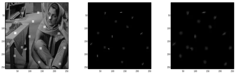
Figure 2: Left to right: image of Barbara, with several locations pi highlighted; Kt(pi,·), for t=
1,2.
stands for Non-Local; in the paper, they proposed settingα=0. In a later paper they add some locality constraints; see Buades et al. (2005b) and Mahmoudi (2005). We wish to emphasize that smoothing with the NL-means filter is not, in any sort of reasonable limit, a 2-d PDE; rather, it is the heat equation on the set of patches of the image!
Note the embedding into 5×5 patches is the same embedding (up to a rotation) as into 5×5 DCT coordinates, and so the weight matrices constructed from these embeddings are the same. On the other hand, if we attenuate small filter responses, the weight matrices for the two filter families will be different.
4.1.2 BOOTSTRAPPING ADENOISER;ORDENOISEDIMAGESGRAPH
Different denoising methods often pick up different parts of the image structure, and create different characteristic artifacts. Suppose we have obtained denoised images f1, ...,fd, from a noisy image f .
To make use of the various sensitivities, and rid ourselves of the artifacts, we could embed pixels
x∈Q intoRd+2by x7→(αx,f1(x), ...,fd(x)). In other words we interpret(fi(x))i=1,...,d as a feature
vector at x. This method is an alternative to “cycle spinning”(Coifman and Donoho, 1995), that is, simply averaging the different denoisings.
In practice, we have found that a better choice of feature vector is fσ(1)(x), ...,fσ(d)(x), whereσ
is a random permutation of{1, ...,d}depending on x. The idea is to mix up the artifacts from the various denoisings. Note that this would not affect standard averaging, since∑fi(x) =∑fσ(i).
4.2 Image Graph Denoising
Once we have the graph W and normalized diffusion K, we use K to denoise the image. The obvious bijection from pixels to vertices in the image graph induces a correspondence between functions on pixels (such as the original image) and functions on the vertices of the graph. In particular the original image can be viewed as a function I on G(I). The functions KtI are smoothed versions
of I with respect to the geometry of G(I). If the graph was simply the standard grid on Q, then
K would be nothing other than a discretization of the standard two-dimensional heat kernel, and KtI would be the classical smoothing of I induced by the Euclidean two-dimensional heat kernel,
1984; Lindeberg, 1994, and references therein). In our context Kt is associated with a scale space induced by G(I), which is thus a nonlinear scale space (in the sense that it depends on the original
1 1 2 1 2 3 1 2 3 4
50 100 150 200 250 50 100 150 200 250 −100 0 100 200 −100 0 100 −100 −50 0 50 100 −500 0 500 −400 −200 0 200 −100 0 100 −400 −200 0 200 400 −200 0 200 −200 0 200 −200 0 200−20 −10 0 10 20 30 −20 −10 0 10
image I). In fact G(I), as described above, is often a point cloud in high-dimensional space, where closeness in those high-dimensional space represents similarity of collections of pixels, and/or of their features, in the original two-dimensional domain of I.
We can balance smoothing by K with fidelity to the original noisy function by setting ft+1= (K ft+βf)/(1+β)whereβ>0 is a parameter to be chosen, and largeβcorresponds to less
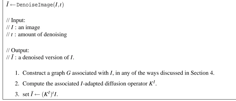
smooth-ing and more fidelity to the noisy image. This is a standard technique in PDE based image process-ing, see Chan and Shen (2005) and references therein. If we consider iteration of K as evolving a heat equation, the fidelity term sets the noisy function as a heat source, with strength determined byβ. Note that even though when we smooth in this way, the steady state is no longer the constant function, we still do not usually wish to smooth to equilibrium. We refer the reader to Figure 4 for a summary of the algorithm proposed.
˜
I←DenoiseImage(I,t)
// Input: // I : an image
// t : amount of denoising // Output:
// ˜I : a denoised version of I.
1. Construct a graph G associated with I, in any of the ways discussed in Section 4. 2. Compute the associated I-adapted diffusion operator KI.
3. set ˜I←(KI)tI.
Figure 4: Pseudo-code for denoising an image
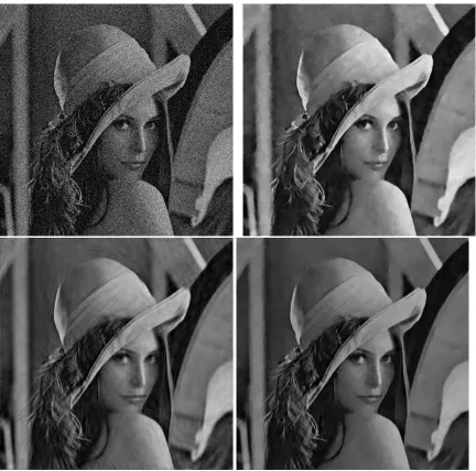
4.3 Examples
Figure 5 displays examples of denoising with a diffusion on an image graph. On the top left of the figure we have the noisy image f0; the noise is N(0, .0244). On the top right of Figure 5, we denoise
the image using a 7×7 NL-means type patch embedding as described in Section 4.1.1. We set
W(k,j) =e−ρ˜81(k,j)2/.3
where ˜ρ81is the distance in the embedding, restricted to 81 point balls in the 2-d metric; that is we take S(k)in Equation (8) to be the 81 nearest pixels to pixel k in the 2-d metric. We then normalize
K=D−1W and denoise the image by applying K three times with a fidelity term of .07; that is,
ft+1= (K ft+.07 f0)/(1.07), and the image displayed is f3. The parameters were chosen by hand.
In the bottom row of Figure 5: on the bottom left, we sum 9 curvelet denoisings. Each curvelet denoisings is a reconstruction of the noisy image f0 shifted either 1, 2, or 4 pixels in the vertical
and/or horizontal directions, using only coefficients with magnitudes greater than 3σ. To demon-strate bootstrapping, or cycle spinning by diffusion, we embed each pixel inR9using the 9 curvelet denoisings as coordinates. We set
Figure 5: 1) Lena with Gaussian noise added. 2) Denoising using a 7×7 patch graph. 3) Denoising using hard thresholding of curvelet coefficients. The image is a simple average over 9 denoisings with different grid shifts. 4) Denoising with a diffusion built from the 9 curvelet denoisings.
where ˜ρ81 is the distance in the embedding, and again we take S(k) in Equation (8) to be the 81 nearest pixels to pixel k in the 2-d metric. We then normalize K=D−1W and denoise the image
by applying K ten times with a fidelity term of .1; that is ft+1= (K ft+.1 f0)/(1.1), and f10 is
5. Application II: Graph Transductive Learning
We apply function adapted approach to the transductive learning problem, and give experimental evidence demonstrating that using function adapted weights can improve diffusion based classifiers. In a transductive learning problem one is given a few “labeled” examples ˜X×F˜ ={(x1,y1), . . . ,
(xp,yp)}and a large number of “unlabeled” examples X\X˜ ={xp+1, . . . ,xn}. The goal is to estimate
the conditional distributions F(y|x)associated with each available example x (labeled or unlabeled). For example ˜F may correspond to labels for the points ˜X , or the result of a measurement at the
points in ˜X . The goal is to extend ˜F to a function F defined on the whole X , that is consistent with
unseen labels/measurements at points in X\X .˜
This framework is of interest in applications where it is easy to collect samples, that is, X is large, however it is expensive to assign a label or make a measurement at X , so only a few la-bels/measurements are available, namely at the points in ˜X . The points in X\X , albeit unlabeled,˜ can be used to infer properties of the structure of the space (or underlying process/probability dis-tribution) that is potentially useful in order to extend ˜F to F. Data sets with internal structures or
geometry are in fact ubiquitous.
If F is smooth with respect to the data, an intrinsic analysis on the data set, such as the one possible by the use of diffusion processes and the associated Fourier and multi-scale analyses, fits very well in the transductive learning framework. In several papers a diffusion process constructed on X has been used for finding F directly (Zhou and Schlkopf, 2005; Zhu et al., 2003; Kondor and Lafferty, 2002) and indirectly, by using adapted basis functions on X constructed from the diffusion, such as the eigenfunctions of the Laplacian (Coifman and Lafon, 2006a,b; Lafon, 2004; Coifman et al., 2005a,b; Belkin and Niyogi, 2003b; Maggioni and Mhaskar, 2007), or diffusion wavelets (Coifman and Maggioni, 2006; Mahadevan and Maggioni, 2007; Maggioni and Mahadevan, 2006; Mahadevan and Maggioni, 2005; Maggioni and Mahadevan, 2005).
We will try to modify the geometry of the unlabeled data so that F is as smooth as possible with respect to the modified geometry. We will use the function adapted approach to try to learn the correct modification.
5.1 Diffusion for Classification
We consider here the case of classification, that is, F takes only a small number of values (compared to the cardinality of X ), say{1, . . . ,k}. Let Ci, i∈ {1, ...k}, be the classes, let Clabi be the labeled
data points in the ith class, that is, Ci={x∈X : ˜˜ F =i}, and letχlabi be the characteristic function
of those Ci, that is,χlabi (x) =1 if x∈Ci, andχlabi (x) =0 otherwise.
A simple classification algorithm can be obtained as follows (Szummer and Jaakkola, 2001):
(i) Build a geometric diffusion K on the graph defined by the data points X , as described in Section 2.2.1.
(ii) Use a power of K to smooth the functionsχlabi , exactly as in the denoising algorithm described above, obtaining functionsχlabi :
χlab
i =Ktχlabi .
The parameter t can be chosen by cross-validation.
(iii) Assign each point x to the class
This algorithm takes into account the influence of the labeled points on the unlabeled point to be classified, where the measure of influence is based on the weighted connectivity of the whole data set. If we average with a power of the kernel we have constructed, we count the number and strength of all the paths of length t to the various classes from a given data point. As a consequence, this method is more resistant to noise than, for example, a simple nearest neighbors (or also a geodesic nearest neighbors) method, as changing the location or class of a small number of data points does not change the structure of the whole network, while it can change the class label of a few nearest neighbors.
For each i, the “initial condition” for the heat flow given by χlabi considers all the unlabeled points to be the same as labeled points not in Ci. Since we are solving many one-vs-all problems, this
is reasonable; but one also may want to set the initial conditionχlab
i (x) =1 for x∈Cilab,χlabi (x) =−1
for x∈Clabj , j6=i, andχlabi (x) =0 for all other x. It can be very useful to change the initial condition to a boundary condition by resetting the values of the labeled points after each application of the kernel. For large powers, this is equivalent to the harmonic classifier of Zhu et al. (2003), where the
χlab
i is extended to the “harmonic” function with given boundary values on the labeled set. Just as
in the image denoising examples, it is often the case that one does not want to run such a harmonic classifier to equilibrium, and we may want to find the correct number of iterations of smoothing by
K and updating the boundary values by cross validation.
We can also use the eigenfunctions of K (which are also those of the Laplacian
L
) to extend the classes. Belkin (2003) suggests using least squares fitting in the embedding defined by the first few eigenfunctions φ1, ...,φN of K. Since the values at the unlabeled points are unknown, we regressonly to the labeled points; so for eachχlabi , we need to solve
argmin{al}
∑
x labeled
N
∑
l=1
ailφl(x)−χlabi (x) 2
,
and extend theχlabi to
χlab
i =
N
∑
l=1 ailφi.
The parameter N controls the bias-variance tradeoff: smaller N implies larger bias of the model (larger smoothness)5 and decreases the variance, while larger N has the opposite effect. Large N thus corresponds to small t in the iteration of K.
5.2 Function Adapted Diffusion for Classification
If the structure of the classes is very simple with respect to the geometry of the data set, then smooth-ness with respect to this geometry is precisely what is necessary to generalize from the labeled data. However, it is possible that the classes have additional structure on top of the underlying data set, which will not be preserved by smoothing geometrically. In particular at the boundaries between classes we would like to filter in such a way that the “edges” of the class function are preserved. We will modify the diffusion so it flows faster along class boundaries and slower across them, by using function-adapted kernels as in (7). Of course, we do not know the class boundaries: the
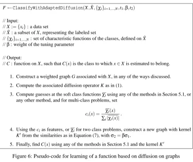
F←ClassifyWithAdaptedDiffusion(X,X˜,{χi}i=1,...,N,t1,β,t2) // Input:
// X :={xi}: a data set
// ˜X : a subset of X , representing the labeled set
//{χi}i=1,...,N : set of characteristic functions of the classes, defined on ˜X //β: weight of the tuning parameter
// Output:
// C : function on X , such that C(x)is the class to which x∈X is estimated to belong. 1. Construct a weighted graph G associated with X , in any of the ways discussed. 2. Compute the associated diffusion operator K as in (1).
3. Compute guesses at the soft class functionsχiusing any of the methods in Section 5.1, or any other method, and for multi-class problems, set
ci(x) = χi(x) ∑i|χi(x)|
.
4. Using the cias features, orχifor two class problems, construct a new graph with kernel K0from the similarities as in Equation (7), withσ2=βσ1.
5. Finally, find C(x)using any of the methods in Section 5.1 and the kernel K0
Figure 6: Pseudo-code for learning of a function based on diffusion on graphs
tions{χi}are initially given on a (typically small) subset ˜X of X , and hence a similarity cannot be
immediately defined in a way similar to (7).
We use a bootstrapping technique. We first use one of the algorithms above, which only uses similarities between data points (“geometry”), to generate the functions χi. We then use these
functions to design a function-adapted kernel, by setting
F
({χi})(x):= (ci(x))i=1,...,k,and then define a kernel as in (7). Here the ci’s are normalized confidence functions defined by
ci(x) = χi
(x) ∑i|χi(x)|
.
In this way, if several classes claim a data point with some confidence, the diffusion will tend to average more among other points which have the same ownership situation when determining the value of a function at that data point. The normalization, besides having a clear probabilistic interpretation when theχi are positive, also achieves the effect of not slowing the diffusion when
there is only one possible class that a point could be in, for example, if a data point is surrounded by points of a single class, but is relatively far from all of them.
since it measures the trade-off between the importance given to the geometry of X and that of the set of estimates{(χi(x))i=1,...,k}x∈X ⊆Rk.
We wish to emphasize the similarity between this technique and those described in Section 4 and especially Section 4.1.2. We allow the geometry of the data set to absorb some of the complexity of the classes, and use diffusion analysis techniques on the modified data set. The parallel with image denoising should not be unexpected: the goal of a function-adapted kernel is to strengthen averaging along level lines, and this is as desirable in image denoising as in transductive learning.
We remark that even if the ci’s are good estimates of the classes, they are not necessarily good
choices for extra coordinates: for example, consider a two class problem, and a function c which has the correct sign on each class, but oscillates wildly. On the other hand, functions which are poor estimates of the classes could be excellent extra coordinates as long as they oscillate slowly parallel to the class boundaries. Our experience suggests, consistently with these considerations, that the safest choices for extra coordinates are very smooth estimates of the classes. In particular, of the three methods of class extension mentioned above, the eigenfunction method is often not a good choice for extra coordinates because of oscillation phenomena; see the examples in Section 5.4.
5.3 Relationship Between Our Methods and Previous Work
In Coifman et al. (2005a) the idea of using the estimated classes to warp the diffusion is introduced. They suggest, for each class Cn, building the modified weight matrix Wn(i,j) =W(i,j)χlabn (i)χlabn (j),
normalizing each Wn, and using the Wnto diffuse the classes. Our approach refines and generalizes
theirs, by collecting all the class information into a modification of the metric used to build the kernel, rather than modifying the kernel directly. The tradeoff between geometry of the data and geometry of the (estimated/diffused) labels is made explicit and controllable.
In Zhu et al. (2003) it is proposed to adjust the graph weights to reflect prior knowledge. How-ever, their approach is different than the one presented here. Suppose we have a two class problem. They add to each node of the graph a “dongle” node with transition probabilityβ, which they leave as a parameter to be determined. They then run the harmonic classifier (Zhu et al., 2003) with the confidence function (ranging from 1 to−1) from a prior classifier as the boundary conditions on all the dongle nodes. Thus their method sets a tension between the values of the prior classifier and the harmonic classifier. Our method does not suggest values for the soft classes based on the prior classifier; rather, it uses this information to suggest modifications to the graph weights between unlabeled points.
5.4 Examples
We present experiments that demonstrate the use of function-adapted weights for transductive clas-sification. We find that on many standard benchmark data sets, classification rate is improved using function-adapted weights instead of “geometry only” weights in diffusion based classifiers.
We use the data sets of Chapelle et al. (2006) and the first 10,000 images in the MNIST data set. At the time this article was written, the respective data sets are available athttp://www.kyb.
tuebingen.mpg.de/ssl-book/benchmarks.htmlandhttp://yann.lecun.com/exdb/mnist/,
with an extensive review of the performance of existing algorithms available at http://www.
kyb.tuebingen.mpg.de/ssl-book/benchmarks.pdf, and athttp://yann.lecun.com/exdb/
All the data sets were reduced to 50 dimensions by principal components analysis. In addition, we smooth the MNIST images by convolving 2 times with an averaging filter (a 3×3 all ones ma-trix). The convolutions are necessary if we want the MNIST data set to resemble a Riemannian manifold; this is because if one takes an image with sharp edges and considers a smooth family of smooth diffeomorphisms of[0,1]×[0,1], the set of images obtained under the family of diffeomor-phisms is not necessarily a (differentiable) manifold (see Donoho and Grimes 2002, and also Wakin et al. 2005). However, if the image does not have edges, then the family of morphed images is a manifold.6
We do the following:
x1. Choose 100 points as labeled. Each of the benchmark data sets of Chapelle et al., has 12 splits into 100 labeled and 1400 unlabeled points; we use these splits. In the MNIST data set we label points 1001 through 1100 for the first split, 1101 to 1200 for the second split, etc, and used 12 splits in total. Denote the labeled points by L, let Ci the ith class, and letχlabi be
1 on the labeled points in the ith class,−1 on the labeled points of the other classes, and 0 elsewhere.
x2. Construct a Gaussian kernel W with k nearest neighbors, σ=1, and normalized so the jth neighbor determines unit distance in the self tuning normalization (Equation 2), where{k,j}
is one of{9,4},{13,9},{15,9}, or{21,15}.
x3. Classify unlabeled points x by supiχlab
i (x), whereχlabi (x)are constructed using the harmonic
classifier with the number of iterations chosen by leave-20-out cross validation from 1 to 250. More explicitly: set g0i =χlab
i . Set gNi (x) = (Kg N−1
i )(x) if x∈/ L, gNi (x) =1 if x∈Ci
T
L,
and gNi (x) =0 if x∈L\Ci, and K is W normalized to be averaging. Finally, setχlabi =gNi (x),
where N is chosen by leave-10-out cross validation between 1 and 250 (Ciand L are of course
reduced for the cross validation).
x4. Classify unlabeled points x by supiχlabi (x), where the χlabi (x) are constructed using least squares regression in the (graph Laplacian normalized) eigenfunction embedding, with the number of eigenfunctions cross validated; that is, for eachχlabi , we solve
argmin{al}
∑
x labeled
N
∑
l=1
ailφl(x)−χi(x) 2
,
and extend theχlabi to
χlab
i =
N
∑
l=1 ailφi.
The φare the eigenfunctions of
L
, which is W normalized as a graph Laplacian, and N is chosen by leave-10-out cross validation.6. For the most simple example, consider a set of n×n images where each image has a single pixel set to 1, and every other pixel set to 0. As we translate the on pixel across the grid, the difference between each image and its neighbor is in a new direction in Rn2
x5. Classify unlabeled points x by supiχlab
i (x), whereχlabi (x)are constructed by smoothingχlabi
with K. More explicitly: set g0i =χlab
i . Set gNi =W gNi −1, where K is W normalized to be
averaging; and finally, letχlab
i =gNi (x), where N is chosen by leave-10-out cross validation
between 1 and 250 (Ciand L are of course reduced for the cross validation).
We also classify the unlabeled points using a function-adapted kernel. Using the χlab
i from the
harmonic classifier at steady state (N=250), we do the following:
x6. If the problem has more than two classes, set
ci(x) =
g250i (x) ∑i|g250i (x)|
,
else, set ci(x) =g250i (x)
x7. Using the ci as extra coordinates, build a new weights ˜W . The extra coordinates are
normal-ized to have average norm equal to the average norm of the original spatial coordinates; and then multiplied by the factorβ, whereβis determined by cross validation from{1,2,4,8}. The modified weights are constructed using the nearest neighbors from the original weight matrix, exactly as in the image processing examples.
x8. Use the function dependent ˜K to estimate the classes as in (x3).
x9. Use the function dependent ˜
L
to estimate the classes as in (x4).x10. Use the function dependent ˜K to estimate the classes as in (x5).
We also repeat these experiments using the smoothed classes as an initial guess, and using the eigenfunction extended classes as initial guess. The results are reported in the Figures 7, 8, and 9. Excepting the data sets g241c, gc241n, and BCI, there is an almost universal improvement in classification rate using function-adapted weights instead of “geometry only” weights over all choices of parameters and all methods of initial soft class estimation.
In addition to showing that function adapted weights often improve classification using diffusion based methods, the results we obtain are very competitive and in many cases better than all other methods listed in the extensive comparative results presented in Chapelle et al. (2006), also available
athttp://www.kyb.tuebingen.mpg.de/ssl-book/benchmarks.pdf. In Figure 10 we attempt
KS FAKS HC FAHC EF FAEF
digit1 2.9 2.2 2.9 2.5 2.6 2.2
USPS 4.9 4.1 5.0 4.1 4.2 3.6
BCI 45.9 45.5 44.9 44.7 47.4 48.7
g241c 31.5 31.0 34.2 32.7 23.1 41.3
COIL 14.3 12.0 13.4 11.1 16.8 15.1
gc241n 25.5 24.7 27.1 25.9 13.9 35.7
text 25.5 23.7 26.3 24.0 26.4 25.4
MNIST 9.4 8.5 9.0 7.9 9.4 8.7
KS FAKS HC FAHC EF FAEF
digit1 2.8 2.2 2.7 2.1 2.6 2.2
USPS 5.2 4.2 5.2 4.0 4.0 3.3
BCI 47.6 47.4 45.0 45.5 48.2 48.6
g241c 30.7 31.2 33.3 32.0 21.7 31.7
COIL 17.2 16.7 16.0 15.1 21.9 19.0
gc241n 23.1 21.6 25.3 22.8 11.1 24.0
text 25.2 23.0 25.5 23.3 26.9 24.0
MNIST 10.0 9.2 10.1 8.7 9.7 8.5
KS FAKS HC FAHC EF FAEF
digit1 3.0 2.3 2.8 2.2 2.6 1.9
USPS 5.0 4.0 5.2 3.9 3.9 3.3
BCI 48.2 48.0 45.9 46.1 47.6 47.9
g241c 30.5 30.4 32.8 31.2 21.2 29.7
COIL 18.0 17.0 16.2 15.2 22.9 19.9
gc241n 24.5 21.7 26.2 23.1 11.1 17.7
text 25.1 22.4 25.7 22.3 25.6 22.9
MNIST 10.3 9.2 10.0 8.9 9.6 8.3
KS FAKS HC FAHC EF FAEF
digit1 3.1 2.6 2.9 2.6 2.0 2.1
USPS 5.6 4.7 5.6 4.4 4.4 3.7
BCI 48.2 48.5 46.3 46.7 48.9 48.5
g241c 28.5 28.2 32.1 29.4 18.0 23.6
COIL 19.8 19.3 19.2 17.9 26.3 24.1
gc241n 21.8 20.5 24.6 21.7 9.2 14.2
text 25.1 22.3 25.6 22.7 25.4 23.2
MNIST 10.8 10.0 10.7 9.7 10.8 10.0
Figure 7: Various classification error percentages. Each pair of columns corresponds to a smoothing method; the right column in each pair uses function adapted weights, with cidetermined
by the harmonic classifier. KS stands for kernel smoothing as in (x5), FAKS for func-tion adapted kernel smoothing as in (x10), HC for harmonic classifier as in (x3), FAHC for function adapted harmonic classifier as in (x8), EF for eigenfunctions as in (x4), and FAEF for function adapted eigenfunctions as in (x9). The Gaussian kernel had k neigh-bors, and the jth neighbor determined unit distance in the self-tuning construction, where counterclockwise, from the top left,{k,j}is{9,4},{13,9},{15,9}, and{21,15}. No-tice that excepting the data sets g241c, gc241n, and BCI, there is an almost universal improvement in classification error with function-adapted weights.
KS FAKS HC FAHC EF FAEF
digit1 2.9 2.4 2.9 2.4 2.6 2.1
USPS 4.9 4.6 5.0 4.6 4.2 3.3
BCI 45.9 47.0 44.9 45.3 47.4 47.8
g241c 31.5 29.3 34.2 29.2 23.1 33.1
COIL 14.3 13.3 13.4 12.4 16.9 16.8
gc241n 25.5 21.3 27.1 22.5 13.9 23.0
text 25.5 24.5 26.3 25.0 26.4 24.6
MNIST 9.4 7.9 9.0 7.7 9.4 7.3
KS FAKS HC FAHC EF FAEF
digit1 2.8 2.2 2.7 2.1 2.6 2.1
USPS 5.2 4.3 5.2 4.0 4.0 3.5
BCI 47.6 48.7 45.0 46.5 48.2 49.1
g241c 30.7 27.9 33.3 27.7 21.7 28.1
COIL 17.2 17.6 16.0 15.5 22.5 20.3
gc241n 23.1 17.9 25.3 19.3 11.1 21.0
text 25.2 23.8 25.5 23.7 26.9 24.5
MNIST 10.0 8.2 10.1 8.2 9.7 7.7
KS FAKS HC FAHC EF FAEF
digit1 3.0 2.5 2.8 2.2 2.6 1.9
USPS 5.0 4.0 5.2 3.9 3.9 3.4
BCI 48.2 48.6 45.9 46.5 47.6 48.1
g241c 30.5 26.9 32.8 27.9 21.2 27.3
COIL 18.0 17.6 16.2 15.8 22.3 21.0
gc241n 24.5 19.7 26.2 20.8 11.1 19.5
text 25.1 22.8 25.7 23.3 25.6 23.4
MNIST 10.3 8.3 10.0 7.9 9.6 7.7
KS FAKS HC FAHC EF FAEF
digit1 3.1 2.6 2.9 2.6 2.0 2.1
USPS 5.6 4.9 5.6 4.2 4.4 4.2
BCI 48.2 49.0 46.3 47.1 48.9 49.0
g241c 28.5 26.0 32.1 26.5 18.0 22.8
COIL 19.8 19.4 19.2 18.3 26.6 23.1
gc241n 21.8 16.5 24.6 17.4 9.2 14.3
text 25.1 22.9 25.6 23.0 25.4 22.8
MNIST 10.8 9.6 10.7 9.2 10.8 8.2
Figure 8: Various classification results, ci determined by smoothing by K. The table is otherwise
organized as in Figure 7.
6. Some Comments on the Benchmarks where Our Methods Do Not Work Well
KS FAKS HC FAHC EF FAEF
digit1 2.9 2.9 2.9 2.6 2.6 2.4
USPS 4.9 4.1 5.0 3.8 4.2 4.1
BCI 45.9 47.1 44.9 46.0 47.4 48.7
g241c 31.5 25.3 34.2 26.7 23.1 23.7
COIL 14.3 13.0 13.4 12.0 16.5 16.6
gc241n 25.5 16.7 27.1 18.2 13.9 14.1
text 25.5 25.1 26.3 25.6 26.4 25.4
MNIST 9.4 7.4 9.0 6.9 9.4 7.9
KS FAKS HC FAHC EF FAEF
digit1 2.8 2.0 2.7 2.1 2.6 2.3
USPS 5.2 3.8 5.2 3.6 4.0 3.4
BCI 47.6 48.1 45.0 46.9 48.2 48.5
g241c 30.7 23.8 33.3 24.7 21.7 21.6
COIL 17.2 17.5 16.0 15.4 22.0 21.5
gc241n 23.1 13.0 25.3 14.1 11.1 11.5
text 25.2 24.8 25.5 24.9 26.9 27.3
MNIST 10.0 7.8 10.1 7.3 9.7 7.4
KS FAKS HC FAHC EF FAEF
digit1 3.0 2.5 2.8 2.2 2.6 2.2
USPS 5.0 4.1 5.2 3.5 3.9 3.2
BCI 48.2 47.5 45.9 45.7 47.6 47.9
g241c 30.5 23.1 32.8 24.1 21.2 21.2
COIL 18.0 17.5 16.2 16.1 22.8 22.1
gc241n 24.5 13.2 26.2 13.9 11.1 11.1
text 25.1 24.3 25.7 24.3 25.6 25.9
MNIST 10.3 8.1 10.0 7.5 9.6 8.6
KS FAKS HC FAHC EF FAEF
digit1 3.1 2.7 2.9 2.5 2.0 2.2
USPS 5.6 4.6 5.6 4.1 4.4 3.6
BCI 48.2 49.0 46.3 47.4 48.9 49.7
g241c 28.5 19.8 32.1 21.5 18.0 18.0
COIL 19.8 19.8 19.2 18.8 26.7 25.8
gc241n 21.8 11.0 24.6 12.0 9.2 9.2
text 25.1 24.1 25.6 24.0 25.4 24.9
MNIST 10.8 8.9 10.7 7.9 10.8 9.4
Figure 9: Various classification results, ci determined by smoothing by eigenfunctions of
L
. Thetable is otherwise organized as in Figure 7.
FAKS FAHC FAEF Best of other methods digit1 2.0 2.1 1.9 2.4 (Data-Dep. Reg.)
USPS 4.0 3.9 3.3 4.7 (LapRLS, Disc. Reg.)
BCI 45.5 45.3 47.8 31.4 (LapRLS)
g241c 19.8 21.5 18.0 13.5 (Cluster-Kernel) COIL 12.0 11.1 15.1 9.6 (Disc. Reg.) gc241n 11.0 12.0 9.2 5.0 (ClusterKernel)
text 22.3 22.3 22.8 23.6 (LapSVM)
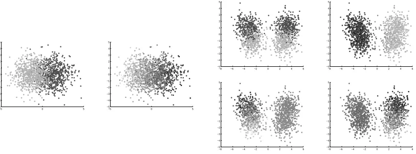
to the cluster center it is nearest to. The boundary between the classes is exactly at the bottleneck between the two clusters; in other words, the geometry/metric of the data as initially presented leads to the optimal classifier, and thus modifying the geometry by the cluster guesses can only do harm. This is clearly visible if one looks at the eigenfunctions of the data set: the sign of the second eigenfunction at a given point is an excellent guess as to which cluster that point belongs to, and in fact in our experiments, often two was the optimal number of eigenfunctions. See figure 11. g241n
−5 0 5
−5 −4 −3 −2 −1 0 1 2 3 4 5
−5 0 5
−5 −4 −3 −2 −1 0 1 2 3 4 5
−8 −6 −4 −2 0 2 4 6 −5 −4 −3 −2 −1 0 1 2 3 4 5
−8 −6 −4 −2 0 2 4 6 −5 −4 −3 −2 −1 0 1 2 3 4 5
−8 −6 −4 −2 0 2 4 6 −5 −4 −3 −2 −1 0 1 2 3 4 5
−8 −6 −4 −2 0 2 4 6 −5 −4 −3 −2 −1 0 1 2 3 4 5
Figure 11: Panel on the left. On the left the lighter and darker points are the two classes for g241c. On the right is the second eigenfunction. Panel on the right. On the top left the lighter and darker points are the two classes for g241n. On the top right is the second eigen-function, then on the bottom the third and fourth eigenfunctions.
is very similar; it is generated by four Gaussians. However, two pairs of centers are close together, and the pairs are relatively farther apart. The classes split across the two fine scale clusters in each coarse scale cluster as in g241c. In this data set, the ideal strategy is to decide which coarse cluster a point is in, and then the problem is exactly as above. In particular, the optimal strategy is given by the geometry of the data as presented. This is again reflected in the simplicity of the classes with respect to eigenfunctions 2, 3, and 4; see figure 11.
While in some sense these situations are very reasonable, it is our experience that in many natural problems the geometry of the data is not so simple with respect to the classes, and function-adapted kernels help build better classifiers.
Our method also was not useful for the BCI example. Here the problem was simply that the initial guess at the classes was too poor.
7. Computational Considerations
nearest) neighbors. This problem is known to be hard even in Euclidean spaceRd, as d increases. The literature on the subject is vast, rather than a long list of papers, we point the interested reader to Datar et al. (2004) and references therein. The very short summary is that for approximate versions of the k-nearest neighbor problem, there exist algorithms which are subquadratic in N, and in fact pretty close to linear. The neighbor search is in fact the most expensive part of the algorithm: once for each point x we know its neighbors, we compute the similarities W (this is
O
(k)for the k neigh-bors of each point), and create the N×N sparse matrix W (which contains kN non-zero entries).The computation of K from W is also trivial, requiring
O
(N)with a very small constant. Apply Kt to a function f on X is very fast as well (for t<<N, as is the case in the algorithm we propose),because of the sparsity of K, and takes
O
(tkN)computations.This should be compared with the
O
(N2)orO
(N3)algorithms needed for other kernel methods, involving the computations of many eigenfunctions of the kernel, or of the Green’s function(I− K)−1.Note that in most of the image denoising applications we have presented, because of the
2-d locality constraints we put on the neighbor searches, the number of operation is linear in the
number N of pixels, with a rather small constant. In higher dimensions, for all of our examples, we use the nearest neighbor searcher provided in the TSTool package, available athttp://www.
physik3.gwdg.de/tstool/. The entire processing of an image as in the examples 256×256 takes
about 7 seconds on a laptop with a 2.2Ghz dual core Intel processor (the code is not parallelized though, so it runs on one core only), and 2Gb of RAM (the memory used during processing is approximately 200Mb).
8. Future Work
We mention several directions for further study. The first one is to use a transductive learning approach to tackle image processing problems like denoising and inpainting. One has at one’s disposal an endless supply of clean images to use as the “unlabeled data”, and it seems that there is much to be gained by using the structure of this data.
The second one is to more closely mimic the function regularization in image processing in the context of transductive learning. In this paper, our diffusions regularize in big steps; also our method is linear (on a modified space). Even though there is no differential structure on our data sets, it seems that by using small time increments and using some sort of constrained nearest neighbor search so that we do not have to rebuild the whole graph after each matrix iteration, we can use truly nonlinear diffusions to regularize our class functions.
9. Conclusions
We have introduced a general approach for associating graphs and diffusion processes to data sets and functions on such data sets. This framework is very flexible, and we have shown two particular applications, denoising of images and transductive learning, which traditionally are considered very different and have been tackled with very different techniques. We show that in fact they are very similar problems and results at least as good as the state-of-the-art can be obtained within the single framework of function-adapted diffusion kernels.
Acknowledgments
The authors would like to thank Francis Woolfe and Triet Le for helpful suggestions on how to improve the manuscript, and to James C. Bremer and Yoel Shkolnisky for developing code for some of the algorithms. MM is grateful for partial support by NSF DMS-0650413 and ONR N00014-07-1-0625 313-4224.
References
M. Belkin. Problems of learning on manifolds. PhD thesis, University of Chicago, 2003.
M. Belkin and P. Niyogi. Using manifold structure for partially labelled classification. Advances in
NIPS, 15, 2003a.
M. Belkin and P. Niyogi. Laplacian eigenmaps and spectral techniques for embedding and clus-tering. In Advances in Neural Information Processing Systems 14 (NIPS 2001), pages 585–591. MIT Press, Cambridge, 2001.
M. Belkin and P. Niyogi. Laplacian eigenmaps for dimensionality reduction and data representation.
Neural Computation, 6(15):1373–1396, June 2003b.
M. Belkin and P. Niyogi. Semi-supervised learning on Riemannian manifolds. Machine Learning, 56(Invited Special Issue on Clustering):209–239, 2004. TR-2001-30, Univ. Chicago, CS Dept., 2001.
Mikhail Belkin and Partha Niyogi. Towards a theoretical foundation for laplacian-based manifold methods. In COLT, pages 486–500, 2005.
P. B´erard, G. Besson, and S. Gallot. Embedding Riemannian manifolds by their heat kernel. Geom.
and Fun. Anal., 4(4):374–398, 1994.
T. Boult, R.A. Melter, F. Skorina, and I. Stojmenovic. G-neighbors. Proc. SPIE Conf. Vision Geom.
II, pages 96–109, 1993.
A. Buades, B. Coll, and J. M. Morel. A review of image denoising algorithms, with a new one.
Multiscale Model. Simul., 4(2):490–530 (electronic), 2005a. ISSN 1540-3459.