The impact of gravity waves rising from convection in the lower atmosphere on the generation and nonlinear evolution of equatorial bubble

(1)

Ann. Geophys., 27, 1657–1668, 2009 www.ann-geophys.net/27/1657/2009/

Annales

Geophysicae

The impact of gravity waves rising from convection in the lower

atmosphere on the generation and nonlinear evolution of equatorial

bubble

E. Alam Kherani1, M. A. Abdu1, E. R. de Paula1, D. C. Fritts2, J. H. A. Sobral1, and F. C. de Meneses Jr.1

1_{Instituto Nacional de Pesquisais Espaciais, Sao Jose dos Campos, SP, Brasil}

2_{NorthWest Research Associates, Colorado Research Associates Division, Boulder, USA}

Received: 24 April 2008 – Revised: 20 March 2009 – Accepted: 20 March 2009 – Published: 7 April 2009

Abstract. The nonlinear evolution of equatorial F-region plasma bubbles under varying ambient ionospheric condi-tions and gravity wave seeding perturbacondi-tions in the bottom-side F-layer is studied. To do so, the gravity wave prop-agation from the convective source region in the lower at-mosphere to the therat-mosphere is simulated using a model of gravity wave propagation in a compressible atmosphere. The wind perturbation associated with this gravity wave is taken as a seeding perturbation in the bottomside F-region to excite collisional-interchange instability. A nonlinear model of collisional-interchange instability (CII) is implemented to study the influences of gravity wave seeding on plasma bub-ble formation and development. Based on observations dur-ing the SpreadFEx campaign, two events are selected for detailed studies. Results of these simulations suggest that gravity waves can play a key role in plasma bubble seeding, but that they are also neither necessary nor certain to do so. Large gravity wave perturbations can result in deep plasma bubbles when ionospheric conditions are not conducive by themselves; conversely weaker gravity wave perturbations can trigger significant bubble events when ionospheric con-ditions are more favorable. But weak gravity wave perturba-tions in less favorable environments cannot, by themselves, lead to strong plasma bubble responses.

Keywords. Ionosphere (Ionospheric irregularities; Plasma waves and instabilities)

1 Introduction

The collisional interchange instability (CII) is believed to play a crucial role in the onset and development of equa-torial spread F (ESF) turbulence (Haerendel, 1973). Radar

Correspondence to: E. Alam Kherani (alam@dae.inpe.br)

observations of ESF reveal the existence of plumes that may penetrate to the topside F-layer and attain very high alti-tudes (Kelley et al., 1981). These plumes are identified as large-scale depletions or plasma bubbles and are believed to be generated by CII and Rayleigh-Taylor instability mech-anism (Sultan, 1996). Numerous theoretical and numerical studies have been performed to assess the linear and non-linear aspects of these complex dynamics (Scannepieco and Ossakow, 1976; Zalesak, 1979; Zargham and Seyler, 1987; Raghavarao et al., 1992; Huang et al., 1993; Keskinen et al., 2003). These studies have revealed the generation of rising bubbles initiated by a seed perturbation at bottomside of a rising F-layer. The seed perturbation used is either in the form of plasma density perturbation (Ossakow et al., 1979; Sekar et al., 1994; Kherani et al., 2005) or of wind pertur-bation, that subsequently cause density perturbation (Huang and Kelley, 1996).

(2)

[image:2.595.50.542.89.189.2]

1658 E. Alam Kherani et al.: Gravity wave and bubble

Table 1. Important ionospheric, bubble and GW activity parameters from the observations.

Events Pre-reversal time (UT) Time of bubble occurrence (UT) Time of periodic modulation

and peak velocity (ms−1) and altitude extension(km) and nature of downward phase propagation

Event 1:

23–24 Oct 21:40, 33 22:10, 600 19–20, weak

24–25 Oct 21:00, 18 22:15, 450 19–20, strong

Event 2: (pre-reversal) (post-reversal)

2–3 Oct (21:20,18) (22:30,12 ) 22:50, 400 19–20, weak

5–6 Oct (21:20,14) (23:10,10) 23:30, 400 19–21, strong (almost 1.25 times stronger than 24–25 Oct)

found that gravity waves with wind amplitude of a few meter per second, horizontal wavelength of few hundred kilome-ters and vertical wavelength of few tens of kilomekilome-ters are a very effective seed mechanism for production of ESF. These studies clearly indicate the potential importance of GWs in the seeding process, but definitive measurements confirming the simultaneous occurrence of GWs and bubble seeding re-mained out of reach.

2 Spread F observations and linear analysis of the CII mechanism

The SpreadFEx campaign was conducted with a primary ob-jective to quantify and understand the importance of GWs, arising from deep tropical convection, on spread F initia-tion at the bottomside F-layer over the Brazilian equatorial region. The campaign period was September to Novem-ber 2005, during which spread F were observed on several nights (Fritts et al., 2009; Abdu et al., 2009). Spread F activ-ity was found to vary day-to-day depending on the ambient ionospheric conditions and GW characteristics (Fritts et al., 2009; Abdu et al., 2009). In a companion paper by Abdu et al. (2009), the digisonde and VHF radar observations of spread F activity during SpreadFEx campaign are analyzed in detail. To study the likely importance of GW contribu-tions to observed spread F activity, Abdu et al. (2009) have presented observations on few selected nights for which it was possible to estimate both mean ionospheric motions and GW contributions independently. The two set of events were chosen to examine the role of GW in the seeding of bubble and they are listed in Table 1.

The first event has two consecutive nights 23–24 October and 24–25 October 2005. On 23–24 October, the peak pre-reversal enhancement (PRE) vertical drift, estimated using the time rate of change of F-layer true heights in 5–8 MHz frequency range of digisonde, is found to be about 33 ms−1 at 21:40 UT and bottomside scale height is found to be about 20 km. In the radar Range-time-intensity (RTI) map, the plume (bubble) first appears at 22:10 UT i.e. 30 min after the pre-reversal peak. The true height variation plot from digisonde does show some degree of wave modulation during

19:00–20:30 UT, an hour and half earlier than the appearance of bubble. However, the modulation does not present any downward phase propagation indicating thereby that the GW activity was rather weak. On the next night 24–25 October, the estimated peak pre-reversal drift and bottomside scale height from digisonde are found to be 18 ms−1at 21:00 UT and 25 km, respectively, indicating less favorable ionospheric conditions for the excitation of CII on this night as compared to previous night. In the RTI map, the plume first appears at 22:15 UT, i.e. 75 min later than pre-reversal peak. A pe-riodic modulation and downward phase propagation in F-layer height variation plot prior to bubble appearance is very prominent during 19:00-20:00 LT indicating the presence of strong GW activity as compared to previous night.

Abdu et al. (2009) have further examined these observa-tions theoretically using linear analysis of CII. The linear analysis solves following governing equation for zonal po-larization electric field:

∂δEx

∂t −γRδEx=sx

where

γR =

−Eox

Bo

−Woy+

g νi

₁

lo

;

sx =

BoUox

lo

_δW

y

κi

−δWx

; 1

lo

=dlogno

dy

andEox,WoyandUox are ambient zonal electric field, verti-cal neutral wind and zonal ion velocity.δW is the perturbed wind associated with GW. This equation is solved for differ-ent background conditions and GW amplitudes to infer the influence of GW seeding in the growth of CII.

(3)

E. Alam Kherani et al.: Gravity wave and bubble 1659 two hours after seeding; (5) Polarization field again grew

ex-ponentially within an hour under less favorable conditions on 24–25 October if GW activity, which is kept low correspond-ing to 23–24 October, was raised three times, correspondcorrespond-ing to 24–25 October.

Another event consisted of two nights 2–3 and 5–6 Octo-ber. On 2–3 October, the ionospheric vertical drift reached a peak of 18 ms−1at 21:20 UT which is followed by a smooth decrease to zero at 22:10 UT. The vertical drift again in-creased (post-reversal) and attained maximum of 16 ms−1at 22:30 UT. The bubble in the RTI first appeared at 22:50 UT during post-reversal after this second peak. The true height variation plot presented weak modulation and weak ten-dency of downward phase propagation which is an indica-tion of weak/marginal GW activity on this night. On 5–6 October, the vertical drift attained maximum of 14 ms−1_at 21:20 UT followed by a downward motion in next 30 min. The ionosphere again moves upward and attained maximum of 12 ms−1within next one hour. The bubble is seen during this post-reversal phase at 23:40 UT. The downward phase propagation prior to the appearance of bubble is prominent during 19:00–21:00 LT indicating the strong GW activity on this night compared to other night. In summary, it can be said that (6) On 2–3 and 5–6 October 2005, ambient iono-spheric conditions are not very different though they were a little less favorable for spread F on 5–6 October; (7) On both nights, the ionosphere undergoes pre-reversal as well as post-reversal phase, (8) On, both nights, bubbles are seen during a second phase of up-lift of ionosphere i.e. during post-reversal phase, (9) On both nights, downward GW phase propagation was noticed in the filtered hF plot from digisonde (Abdu et al., 2009). However, on 2–3 October 2005, the GW activity was weaker than on 5–6 October 2005, (10) Linear growth analysis revealed that polarization field grows exponentially on 2–3 October, (11) It further show weaker growth for a case where ambient conditions correspond to 5–6 October and GW amplitude correspond to 2–3 October, (12) It again revealed exponential growth on night 5–6 October when GW amplitude is raised three times than its amplitude on 2–3 Oc-tober.

Linear analysis presented in a companion paper (Abdu et al., 2009) only ensures initial growth of CII without taking into account temporal variations of ambient parameters such as vertical drift and rapid varying density owing to the insta-bility itself. These variations may or may not allow expo-nential growth to continue depending on the nature of vari-ations. This aspect can be examined only with a nonlinear simulation of CII. The two sets of events described above of-fer ideal conditions to study the effects of GW seeding under varying ionospheric conditions and may be helpful in bring-ing out additional features concernbring-ing seedbring-ing mechanism. Hence, we present here several nonlinear simulations of CII for different background conditions and GW amplitudes that correspond as closely as possible to those observed on 23–24 October/24–25 October and 2–3 October/5–6 October 2005.

The model employed for our study is described in Sect. 3. Section 4 provides a discussion of the model results and their implications for GW seeding of ESF and equatorial plasma bubbles, and our conclusions are presented in Sect. 5.

3 Model equations and algorithms

We adopt the following set of equations to study the collisional-interchange instabilities in the equatorial F-region (Kherani et al., 2004):

∂n

∂t +∇.(nue)= −βn−αn

2 ₍₁₎

∇.J =e∇.[n(ui−ue)] =0. (2)

ui,e=

κi,e

1+κ_i,e2 vi,e× ˆb+

1

1+κ_i,e2 vi,e (3)

where

vi,e =

−c2_si,e νi,en

∇logn+ g

νi,en

+bi,eE+W

The subscripts “e” and “i” refer to the electrons and ions, re-spectively. Equations (1) and (2) are the electron continuity and divergence free current (J) equations respectively, while

u_i,ein Eq. (3) are the ion and electron’s steady state veloci-ties. The plasma is assumed to be charge-neutral(ne=ni=n), and it is ensured by Eq. (2). The terms in the right-hand side of Eq. (1) correspond to the chemical loss of electrons by charge exchange process (β) and dissociative recombination process (α) respectively. The notationsκi,erepresent the ra-tios of the gyro frequencies, i,e, to collision frequencies,

(4)

:

1

43ms

-150

0

150 Zonal distance, km

230

330

430

530 Altitude, km

(a) Perturbed GW wind,

W

o

0

.

7ms

-150

0

150 Zonal distance, km

[image:4.595.130.465.58.411.2]

(b) Perturbed ion velocity,

u

i

Fig. 1.(a) The distribution of amplitudeδWoof GW (b) and the perturbed ion velocityδuiin the F region at t=0.

Fig. 1. (a) The distribution of amplitudeδWoof GW (b) and the perturbed ion velocityδuiin the F-region att=0.

fieldE=Eo+δE=Eo−∇8, the divergence-free current den-sity Eq. (2) is reduced to the following equation for the per-turbed potential (8) in the F-region (Kherani et al., 2004):

∇28+∂log(κin)

∂x ∂8

∂x +

∂log(κin)

∂y ∂8

∂y =s (4)

and ion continuity Eq. (1) can be written as follows:

∂n

∂t +F(n, 8).∇logn=Ren (5)

where

Re=

₁

β +

1

αn(t )

−1

is the effective recombination rate and

F =n(uo+δu); δu= 1

κi

δW −κi

∇8 Bo

× ˆbo (6) is the particle flux. Hereuoandδuare steady-state ambient and pertubed ion velocity respectively. In Eq. (4),sis given by following expression:

s= −Bo

_g

νin

−Exo

B −Wy

_∂_log_n

∂x

or

s= −Bo(γR+δγ )lo

∂logδn

∂x (7)

where

γR=

_g

νin

−Eox

Bo

−Woy

₁

lo

;

δγ = −δWy

lo 1

lo

= dlogno

dy (8)

Equations (4–5) form a coupled closed system of equations for CII in the F-region. In the expression of s, γR can be recognized as the growth rate of CII.Wo appearing in γR represents the background neutral wind and its effects are ig-nored in present study. The fluctuating perturbed windδW

(5)

E. Alam Kherani et al.: Gravity wave and bubble 1661

2 :

0

1

2

3

₁₀11

m

3

4

5

6

7

180

380

580 Altitude, km

(a) Ambient density,

n

o

Case 1a

Case 1b/1c

Case 2a/2b/2c/2d

0 3000

6000

t, seconds

-20

0

20 u

oy

, m/

s

(b) Ambient velocity

[image:5.595.128.466.64.414.2]

Case 1a

Case 1b/1c

Case 2a

Case 2b

Case 2c/2d

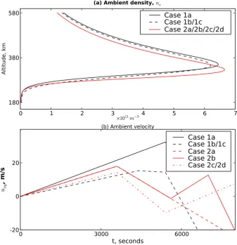
Fig. 2. (a) An altitude profile of initial ionospheric density and (b) temporal variation of ambient vertical velocity chosen for different cases

under event 1 and 2. Case 1a, 1c, 2b, 2d represent ambient ionospheric conditions and GW amplitude as close as possible to the observed spread F nights 23-24, 24-25, 02-03 and 05-06 Oct 2005 respectively.

Fig. 2. (a) An altitude profile of initial ionospheric density and (b) temporal variation of ambient vertical velocity chosen for different cases

under event 1 and 2. Case 1.a, 1.c, 2.b, 2.d represent ambient ionospheric conditions and GW amplitude as close as possible to the observed spread F nights 23–24, 24–25, 2–3 and 5–6 October 2005, respectively.

density according to the continuity equation (Eq. 5) and it modifies the growth of the instabilityγRby introducing per-turbationδγ inswhich appears in Poisson equation (Eq. 4). With a chosen seeding perturbation of amplitudeδW asso-ciated with GW and the ambient ionospheric conditions (that are described below and in Figs. 1–2), the continuity Eq. (5) is solved using the Crank-Nicholson implicit scheme at first (Kherani et al., 2004). The potential Eq. (4) is then solved us-ing the Successive-Over-Relaxation algorithm with the per-turbed density. This solution is again substituted into Eq. (5) to obtain a time-evolved density and this loop continues till maximum upward velocity of ion becomes 1000 ms−1_{. The} simulation plane consists of x and y boundaries in zonal and vertical directions respectively. The x-boundaries are lo-cated at±150 km with 2.5 km grid resolution and periodic boundary conditions are imposed on these boundaries. The y-boundaries are located at 180 km and 580 km with 2.5 km grid resolution. The transmittive boundary condition onn

and the Neumann boundary condition on8are imposed on

these boundaries. These boundary conditions are the same as those chosen by Sekar et al. (1994) and sufficient to en-sure the vanishing current density across the lower bound-ary provided that the ambient ionosphere is invariant at the boundary.

(6)

[image:6.595.55.281.86.228.2]

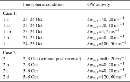
Table 2. Numerical simulation under different events.

Ionospheric condition GW activity

Case 1:

1.a 23–24 Oct δwx,y=40, 20 ms−1

1.aa 23–24 Oct δwx,y=20, 10 ms−1

1.ab 23–24 Oct δwx,y=4, 2 ms−1

1.b 24–25 Oct δwx,y=40, 20 ms−1

1.c 24–25 Oct δwx,y=100, 50 ms−1

Case 2:

2.a 2–3 Oct (without post-reversal) δwx,y=40, 20ms−1

2.b 2–3 Oct δwx,y=40, 20 ms−1

2.c 5–6 Oct δwx,y=40, 20 ms−1

2.d 5–6 Oct δwx,y=120, 60 ms−1

are chosen to be two and four times larger than the scale height at each altitude. Fixing these wavelengths, the fre-quency (ω) of the GW is obtained from the dispersion re-lationω2λ2_x=(N2−ω2)λ2_ywhereN is the Brunt-Vaisala fre-quency. This is one among few options by which the GW’s parameters can be selected. An alternative approach is to fix theλyandωand calculate theλxfrom above dispersion rela-tion (Abdu et al., 2009). The wave frequency estimated using the first approach is found to be in the range 10–60 min, de-pending on the altitude. The wave resides in the equatorial plane (x-y) perpendicular to magnetic field and propagates obliquely at an elevation angle 84◦. It means that the wind fluctuations associated with such GWs make an angle of 6◦ from horizontal. The fluctuating windδW_oassociated with the GW is shown in Fig. 1a. It can be seen thatδWo maxi-mizes in the F-region and it is dominantly horizontal having horizontal wavelength in the range of 200–300 km and verti-cal wavelength in the range of 100–150 km. The maximum horizontal and vertical winds associated with GW are of or-der of 40 ms−1_{and 10 ms}−1_{, respectively. This GW,} intro-duces a perturbationδuin the ion velocityuo according to Eq. (6). This perturbed velocity is computed usingδWterms in Eq. (6) and it is plotted in Fig. 1b. It is noted thatδuis dominantly vertical with a magnitude of 0.5–1 ms−1in the bottomside F-region.

A SpreadFEx companion paper by Fritts and Vadas (2008) employed the ray tracing methods of Vadas and Fritts (2004) to assess GW Doppler shifting by thermospheric winds, pref-erential penetration and dissipation, and selection of those GW periods and spatial scales achieving the highest altitudes for various thermospheric winds and solar conditions and ar-bitrary GW sources in the lower atmosphere. They suggested that those GWs achieving the largest amplitudes will neces-sarily play the major roles in ionospheric plasma processes and that such GWs typically have relatively high intrinsic fre-quencies (the observed and the intrinsic periods being∼10 to 60 min and ∼10 to 30 min, respectively) and large hori-zontal and vertical scales (dominant horihori-zontal and vertical wavelengths being ∼150 to 500 km and ∼150 to 300 km,

respectively, for solar conditions representative of Spread-FEx condition). These theoretical estimates appear to be in good agreement with the typical GW periods observed dur-ing the SpreadFEx campaign that were found to be in the

∼15–60 min range near 300 km (Abdu et al., 2009; Fritts et al., 2009). The longer wavelength GWs that are expected to reach F-region altitudes, are also expected to achieve hori-zontal velocities in the range of 10–100 ms−1or higher, de-pending on propagation conditions, specific scales, and prox-imity to their sources. Corresponding vertical component is typically somewhat smaller, but may also attain similar am-plitudes near altitudes at which they approach evanescence. It can be noted that the frequency, wavelengths and ampli-tudes of GW obtained in present investigation (Fig. 1a–b) fall in the same range as suggested by Fritts and Vadas (2008).

4 Results and discussion

Using simulation model described above, two events, which are discussed in Sect. 2 and listed in Table 1, are studied. The First event set consists of 23–24/24–25 October 2005 and second event set consists of 2–3/5–6 October 2005. In next two subsections, we present the numerical results corre-sponding to these two events respectively.

4.1 Event 1: 23–24 and 24–25 October 2005

On 23–24 October/24–25 October, the modulation and downward phase propagation in the true height vs. time plot are seen mainly during 19:00–21:00 UT and pre-reversal en-hancement peak occurred almost an hour or more later (Abdu et al., 2009). On this basis, our simulation (t=0 s) begins at 20:00 LT when GW activities are observed and when the ionosphere upward drift is small. The amplitude of GW on two nights are derived using observed time variation of bot-tomside F-layer height (hF). The time rate of change ofhF

at given time represents perturbed upward ion velocityδu. For one hour periodic modulation observed during 19:00– 21:00 UT, this time rate is estimated on each night and the corresponding wind perturbationδWx≈κiδuyis obtained us-ing Eq. (6). It is found that estimatedδuis of the order of 1 ms−1and 2.5 ms−1on 23–24 October and 24–25 October, respectively. On this basis, we have chosenδW=δWo and

δW=2.5δWofor 23–24 October and 24–25 October, respec-tively, whereδWo is shown in Fig. 1a. The initial density profile and temporal profile ofuoy=−Eox/Bofor these cases are shown in Fig. 2a and b. These profiles are deduced from the digisonde observations presented in Abdu et al. (2009). On the basis of ambient ionospheric conditions and GW ac-tivity, we consider following cases within the Event 1 (they are also listed in Table 2):

(7)

:

3

180

380

580 Altitude, km

41.666664

1.0 2.0 2.0 3.0 3.0 4.0 4.0 5.0 5.0 6.0 6.0

(a) Case 1a

41.666664

0.8 1.6 1.6 2.4 2.4 3.2 3.2 4.0 4.0 4.8 4.8 5.6 5.6

(b) Case 1b

41.66666

0.8 1.6 1.6 2.4 2.4 3.2 3.2 4.0 4.0 4.8 4.8 5.6 5.6

(c) Case 1c

180

380

580 Altitude, km

5563.4609

0.8 1.6 2.43.2 3.2 4.0 4.0 4.8 4.8 5.6 5.6

4114.8613

0.8 1.62.4

2.4 3.2 3.2 4.0 4.0 4.8 4.8 5.6 5.6

5989.4175

0.8 1.6 2.4 2.4 3.2 3.2 4.0 4.0 4.8 4.8 5.6 5.6

-150

0

150

180

380

580 Altitude, km

5959.4834

0.8 1.6 2.43.2 3.2 4.0 4.0 4.8 4.8 5.6 5.6

-150

0

150 Zonal disance, km

6686.3481

0.8 1.6 1.6 2.4 2.4 3.2 3.2 4.0 4.0 4.8 4.8 5.6 5.6

-150

0

150

[image:7.595.128.466.60.415.2]

7043.9009

0.8 1.6 2.4 2.4 3.2 3.2 4.0 4.0 4.8 4.8 5.6 5.6

Fig. 3.Event 1: The evolved iso-density contours in the simulation plane for (a) case 1.a (b) case 1.b and (c) case 1.c.

Fig. 3. Event 1: The evolved iso-density contours in the simulation plane for (a) Case 1.a (b) Case 1.b and (c) Case 1.c.

Case 1.b: Ambient condition corresponding to 24-25 Oct, and GW amplitude corresponding to 23–24 October, i.e.

δW=δWo;

Case 1.c: Ambient condition and GW amplitude correspond-ing to 24–25 October, i.e.δW=2.5δWo;

Case 1.aa and 1.ab: Ambient conditions corresponding to 23–24 October and GW amplitude is lowered by factor 0.5 and 0.2 from its amplitude on 23–24 October.

The results corresponding to the different cases under event 1 are shown in Figs. 3–4. In Fig. 3, the iso-density con-tours (IDCs) are shown for Case 1.a (left-panels), Case 1.b (middle-panels) and Case 1.c (right panels) during the evo-lution of CII in each case. For each case, the evoevo-lution of CII at different time (written on the top of each panel) are presented. It is evident that the initial perturbations grow as rapidly rising plasma bubbles in Cases 1.a and 1.c, but not in Case 1.b, highlighting the importance of enhanced GW activity that gives rise to the plasma bubble in Case 1.c un-der less favorable ambient conditions than in Case 1.a. This aspect is more clear in Fig. 4 where the maximum upward

velocity inside a depletion is plotted for Case 1.a–1.c. It is known from earlier simulation studies that large upward ve-locity inside a depletion is an indication of nonlinear growth of CII (Sekar et al., 1994). The upward velocity is computed from the solution of Eq. (4) using the following expression:

δuy= −

δEx Bo = 1 Bo ∂8 ∂x

(8)

4 :

0 1000 2000 3000 4000 5000 6000 7000

Time, seconds

0 50 100 150 200

Velocity, m/s

Evolution of maximum upward velocity of the depletion

uy Case 1a

[image:8.595.50.284.63.304.2]

Case 1aa Case 1ab Case 1b Case 1c

Fig. 4.Event 1: The growth of maximum upward velocity of depletion for Case 1.a-1.c.

Fig. 4. Event 1: The growth of maximum upward velocity of

deple-tion for Case 1.a–1.c.

marginal growth and no-growth tendency. It means that in spite having highly favorable ambient conditions on 23–24 October, the bubble growth is substantially reduced if the amplitude of seeding GW is lowered. It means that the GW amplitude above certain threshold is needed to seed the in-stability that can develop into bubble. It is then noted that in spite the largeδWon 24–25 October than on 23–24 October, CII growth is much faster on 23–24 October 2005. This is attributed to the ambient ionospheric conditions such as ver-tical drift, density gradient, and F-layer height that dictate the growth of CII, being less favorable on 24–25 October 2005. We note that though GW is needed to seed or initiate the in-stability, its impact on the growth is dictated by the ambient ionospheric conditions. In essence, all it can be said that the GW with amplitude larger than certain threshold is a suitable seeding for the CII. However, it may or may not cause the growth of CII depending on the ambient ionospheric condi-tions. The nonlinear features presented in Figs. 3–4 are in ac-cord with the results obtained using linear analysis by Abdu et al. (2009).

Afore-mentioned behavior of CII under varying GW ac-tivities can be discussed qualitatively by analyzing the conti-nuity Eq. (5) and source functionsin Poisson Eq. (4). The order of density perturbation caused by the GW wind can be obtained from Eq. (4) as follows:

ωδn∼noδuy/λx; or

δn no

∼ νin

i

τ δwx

λx

= νin

i

δwx

vph

whereτ=1/ωandλxare the time-period and wavelength as-sociated with GW andvphis its phase velocity in x-direction. Forτ=30 min,λx=200 km andδwx=40 ms−1,δn/no∼0.5% i.e. the F-region ionospheric density is perturbed by 0.5– 1% from its ambient value caused by the GW described in Fig. 1a–b. This perturbation appear in source function s

which is given by Eq. (7) and can also be written as follows:

s=Bo(γR+δγ )

lo

δlx where

1

δlx

= ∂logn

∂x ∼

1

λx

δn no

∼ τ

λ2 x

νin

i

δwx

Thusscan be written as follows:

s∼Bo

γR−

δwy

lo

λx

δwx

vph

In Case 1.a,δwis small but sinceγRis large, the source func-tionsis sufficiently large for instability to grow. In Case 1.c,

γR is smaller (almost by factor 2) than its value in Case 1.a. However,δwis larger (by factor 2) than its value in Case 1.c owing to enhanced GW activity. Thus the value of “s” may still remain sufficiently large for the growth of bubble for Case 1.c. For Case 1.b, bothγR andδware small implying smallsand insignificant growth of CII.

[image:8.595.307.462.158.293.2]

(9)

: 5

3000 3500 4000 4500 5000 5500 6000

Time, seconds

0 50 100 150 200

Velocity, m/s

Evolution of maximum upward velocity of the depletion

uy

[image:9.595.49.287.62.303.2]

With GW effects in

R

Without GW effects in

R

Fig. 5.Event 1: The growth of maximum upward velocity of depletion for case without GW windδWeffects on the growth rateγR. The ionospheric conditions and GW activities are kept same as in Case 1c. For comparison, the growth of velocity for Case 1.c is also plotted.

de-pletion for case without GW windδW effects on the growth rate γR. The ionospheric conditions and GW activities are kept same as

in Case 1.c. For comparison, the growth of velocity for Case 1.c is also plotted.

4.2 Event set 2: 02-03 and 05-06 October 2005

These are the post-reversal events where deceleration (on 2–3 October) or reversal (5–6 October) of upward drift of iono-sphere after pre-reversal is followed by upward drift again. Similar to event 1, the simulation begins at 20:00 LT for event 2, when GW activities are observed and when iono-sphere upward drift is small. The GW amplitudes on the two nights are determined from digisonde observations as it was done for event 1 andδW is found to be equal toδWo and 3δWoon 2–3 October and 5–6 October, respectively. To study this event, we have examined the following cases: Case 2.a: Ambient ionosphere conditions corresponding to 2–3 October but without post-reversal increase in vertical drift and GW amplitudeδW=δWo,

Case 2.b: Ambient ionosphere conditions corresponding to 2–3 October including the post-reversal increase in vertical drift and GW amplitudeδW=δWo,

Case 2.c: Ambient ionosphere conditions corresponding to 5–6 October and GW amplitudeδW=δWo.

Case 2.d: Ambient ionosphere conditions corresponding to 5–6 October and GW amplitudeδW=3δWo.

The Ionospheric number density profile used in all the cases are same and shown in Fig. 2a. The corresponding time vari-ation of ambient vertical driftuoyfor these cases are shown in Fig. 2b. In Fig. 6, the growth of maximum velocity of the

6 :

0 1000 2000 3000 4000 5000 6000 7000 8000 9000

Time, seconds

0 50 100 150 200 250 300

Velocity, m/s

Evolution of maximum upward velocity of the depletion uy

[image:9.595.309.540.66.303.2]

Case 2a Case 2b Case 2c Case 2d

Fig. 6.Event 2: The growth of maximum upward velocity of depletion for Case 2.a-2.d

deple-tion for Case 2.a–2.d

(10)

:

7

180

380

580 Altitude, km

41.666664

1.0 2.0

2.0

3.0 3.0

4.0 4.0

5.0 5.0

6.0 6.0

(a) Case 2b

41.666664

1.0 2.0

2.0

3.0 3.0

4.0 4.0

5.0 5.0

6.0 6.0

(b) Case 2d

180

380

580 Altitude, km

7267.9468

0.8 1.62.4

2.4

3.2

4.0

4.8

5.6

7998.0469

0.8

1.6

2.4 2.4

3.2

4.0

4.8

5.6

-150

0

150 Zonal distance, km

180

380

580 Altitude, km

7949.4282

0.8 1.62.4 2.4

3.2 3.2

4.0

4.8 4.8

5.6

-150

0

150 Zonal distance, km

8951.4609

0.8 1.6

1.6

2.4 2.4

3.2

4.0 4.0 4.8

4.8

[image:10.595.129.464.62.413.2]

5.6 5.6

Fig. 7.Event 2: The evolved iso-density contours in the simulation plane for (a) Case 2b and (b) Case 2d.

Fig. 7. Event 2: The evolved iso-density contours in the simulation plane for (a) Case 2.b and (b) Case 2.d.

occasions, bubbles evolved much later caused by the second peak in the vertical drift. This kind of behavior of bubble was simulated earlier by Sekar and Kelley (1998) to explain the late emergence of plume over Jicamarca.

5 Conclusions

The influences of gravity wave wind perturbations on the evolutions of plasma bubbles are examined for varying ambi-ent ionospheric conditions deduced from observations during the SpreadFEx campaign performed in Brazil from Septem-ber to NovemSeptem-ber 2005. Nonlinear simulations of collisional interchange instability are performed to accomplish this task. The gravity waves (GW) are assumed to be launched from convective regions in the troposphere. Their upward propa-gations to thermospheric height are studied using a gravity wave propagation model presented in an earlier work. The gravity wave amplitude in the F-layer is found to be of or-der of tens of meter per second for an assumed amplitude of 0.5 cm s−1 at 10 km altitude in troposphere. Our results

demonstrate that the gravity wave seeding can excite the col-lisional interchange instability and give rise to plasma bub-bles, depending on ambient ionospheric conditions. We have presented a detailed study of two event sets with varying ionospheric conditions and gravity wave amplitudes for these studies.

The first event set corresponds to 23–24 October and 24– 25 October 2005 for which gravity wave amplitudes are found to be low and high, respectively. The ambient iono-spheric conditions are less favorable for the generation of CII on 24–25 October. It is found that a low gravity wave ampli-tude corresponding to 23–24 October cannot give rise to a plasma bubble for less favorable ambient conditions repre-senting 24–25 October However, under same less favorable conditions, a bubble can grow if the gravity wave amplitude is increased to a value corresponding to that which charac-terized the event of 24–25 October. This result is a clear indication of impact of gravity wave seeding on the growth of plasma bubbles.

(11)

E. Alam Kherani et al.: Gravity wave and bubble 1667 conditions are not very different, though they are little less

favorable on 5–6 October 2005. The GW activity was noted on both days, though it was stronger on 5–6 October. These are the post-reversal events where deceleration or reversal of upward drift of ionosphere after its pre-reversal peak is followed by upward drift again. Our numerical simulation of this event reveals that bubbles are generated during post-reversal upward motion of ionosphere on both the nights. The bubbles growth would not have occurred on 5–6 October if the gravity wave amplitude is lowered to its value on 2–3 October, due to the rapid downward motion of ionosphere after the pre-reversal peak.

Summarizing, our nonlinear simulations of collisional-interchange instabilities for F-layer environments and GW perturbations guided by measurements during the Spread-FEx campaign appear to confirm the suggestions by Fritts et al. (2008b) and the linear plasma instability analysis by Abdu et al. (2009) that GWs can attain sufficiently large amplitudes to significantly enhance CII growth rates and the seed plasma bubbles extending to much higher altitudes. Our sensitivity studies also indicate an important role for gravity waves in the seeding process and suggest that spread F dynamics can likely not be understood fully without sensitivity to poten-tial gravity wave contributions to the state of the ionosphere at the time of bubble seeding. It is important to mention that more general numerical studies have been performed in the past on the GW seeding mechanism (Huang et al., 1993; Huang and Kelley, 1996). The present study is rather an at-tempt to provide supportive evidences of gravity wave seed-ing mechanism on the basis of a few observed events and their numerical simulations.

Acknowledgements. The authors wish to acknowledge the supports

from FAPESP through the process 07/00104-0, project 1999/00437-0, and CNPq through grants no 502804/2004-1, 500271/2003-8. The SpreadFEx field program and supporting data analyses and modeling were also supported by NASA contracts NNH04CC67C and NAS5-02036 and AFOSR contract FA9550-06-C-0129.

Topical Editor U.-P. Hoppe thanks S. Saito and another anony-mous referee for their help in evaluating this paper.

References

Abdu, M., Alam Kherani, E., Batista, I. S., de Paula, E. R., and Fritts, D. C.: Gravity wave influences on plasma instability growth rates based on observations during the Spread F Experi-ment (SpreadFEx), Ann. Geophys., in press, 2009.

Fritts, D. C., Abdu, M. A., Batista, B. R., et al.: Overview and summary of spread F experiment (spreadFEx), Ann. Geophys., in review, 2009.

Fritts, D. C. and Vadas, S. L.: Gravity wave penetration into the thermosphere: sensitivity to solar cycle variations and mean winds, Ann. Geophys., 26, 3841–3861, 2008a,

http://www.ann-geophys.net/26/3841/2008/.

Fritts, D. C., Vadas, S. L., Riggin, D. M., Abdu, M. A., Batista, I. S., Takahashi, H., Medeiros, A., Kamalabadi, F., Liu, H.-L.,

Fejer, B. G., and Taylor, M. J.: Gravity wave and tidal influ-ences on equatorial spread F based on observations during the Spread F Experiment (SpreadFEx), Ann. Geophys., 26, 3235– 3252, 2008b, http://www.ann-geophys.net/26/3235/2008/. Hysell, D. L., Kelley, M. C., Swartz, W. E., and Woodman, R. F.:

Seeding and layering of equatorial spread F by gravity waves, J. Geophys. Res., 95, 17253–17260, 1990.

Huang, C. S., Kelley, M. C., and Hysell, D. L.: Nonlinear Rayleigh-Taylor instabilities, atmospheric gravity waves, and equatorial spread F, J. Geophys. Res., 98, 15631–15642, 1993.

Huang, C. S. and Kelley, M. C.: Nonlinear evolution of equatorial spread F 4. Gravity waves, velocity shear and day-to-day vari-ability, J. Geophys. Res., 101, 24521–24532, 1996.

Kelley, M. C., Larsen, M. F., LaHoz, C., and McClure, J. P.: Gravity wave initiation of equatorial spread F: A case study, J. Geophys. Res., 86, 9087–9100, 1981.

Kelley, M. C., LaBelle, J., and Kudeki, E.: The Condor equatorial spread F campaign: Overview of the results of large scale mea-surements, J. Geophys. Res., 91, 5487–5503, 1986.

Keskinen, M. J., Ossakow, S. L., and Fejer, B. G.:

Three-dimensional nonlinear evolution of equatorial

iono-spheric spread-F bubbles, Geophys. Res. Lett., 30, 1855, doi:10.1029/2003GL017418, 2003.

Kherani, E. A., de Paula, E. R., and Bertoni, F. C. P.: Effects of the fringe field of Rayleigh-Taylor instability in the equa-torial E and valley regions, J. Geophys. Res., 109, A12310, doi:10.1029/2003JA010364, 2004.

Kherani E. A., Mascarenhas, M., Sobral, J. H. A., de Paula, E. R., and Bertoni, F. C.: A three dimension simulation model of col-lisional interchange instability, Space Sci. Rev., 121, 253–269, 2005.

Kherani E. A., Lognonne, P., Nishant Kamath, Crespon, F., and Garcia, R.: Response of the Ionosphere to the seismic trigerred acoustic wave: electron density and electromagnetic fluctuations, Geophys. J. Int., 176, 1–13, 2009.

McClure, J. P., Singh, S., Bamgboye, D. K., Johnson, F. S., and Kil, H.: Occurrence of equatorial F-region irregularities: Evidence for tropospheric seeding, J. Geophys. Res., 103, 29119–29135, 1998.

Ogawa, T., Ostuka, Y., Shiokawa, K., Saito, A., and Nishioka, M.: Ionospheric disturbances over Indonesia and their possible asso-ciation with atmospheric gravity waves from the troposphere, J. Meteorological Society of Japan, 84A, 327–342, 2006.

Ossakow, S. L., Zalesak, S. T., McDonald, B. E., and Chaturvedi, P. K.: Nonlinear equatorial spread F: Dependence on altitude of the F peak and bottom-side background electron density gradient scale length, J. Geophys. Res., 84, 17–29, 1979.

Raghavarao, R., Sekar, R., and Suhasini, R.: Nonlinear numerical simulation of equatorial spread F - Effects of winds and electric fields, Adv. Space Res., 12, 227–230, 1992.

Rottger, J.: Equatorial spread F by electric fields and atmospheric gravity waves generated by thunderstorms, J. Atmos. Terr. Phys., 43, 453–462, 1981.

Scannapieco, A. J. and Ossakow, S. L.: Nonlinear equatorial spread F, Geophys. Res. Lett., 3, 451–454, 1976.

Sekar, R., Suhasini, R., and Raghavarao, R.: Effects of vertical winds and electric fields in the nonlinear evolution of equatorial spread F, J. Geophys. Res., 99, 2205–2213, 1994.

(12)

and zonal electric field patterns on nonlinear equatorial spread F evolution, J. Geophys. Res., 103(A9), 20735–20747, 1998. Singh, S., Johnson, F. S., and Power, R. A.: Gravity wave seeding

of equatorial plasma bubbles, J. Geophys. Res., 102, 7399–7410, 1997.

Sultan, P.: Linear theory and modelling of the Rayleigh-Taylor in-stability leading to the occurrence of equatorial spread F, J. Geo-phys. Res., 101, 26875–26891, 1996.

Vadas, S. L.: Horizontal and vertical propagation, and dissipation of gravity waves in the thermosphere from lower atmospheric and thermospheric sources, J. Geophys. Res., 112, A06305, doi:10.1029/2006JA011845, 2007.

Vadas, S. L. and Fritts, D. C.: Thermospheric responses to gravity waves arising from mesoscale convective complexes, J. Atmos. Solar Terres. Phys., 66, 781–804, 2004.

Zalesak, S. T.: Fully multidimensional flux-corrected transport al-gorithms for fluids, J. Comp. Phys., 31, 335–362, 1979. Zargham, S. and Seyler, C. E.: Collisional Interchange