Long-term variations of the mesospheric wind field at mid-latitudes

Received: 12 June 2007 – Accepted: 26 July 2007 – Published: 29 August 2007

Abstract. Continuous MF radar observations at the station Juliusruh (54.6◦N; 13.4◦E) have been analysed for the time interval between 1990 and 2005, to obtain information about solar activity-induced variations, as well as long-term trends in the mesospheric wind field. Using monthly median values of the zonal and the meridional prevailing wind components, as well as of the amplitude of the semidiurnal tide, regres-sion analyses have been carried out with a dependence on solar activity and time. The solar activity causes a significant amplification of the zonal winds during summer (increasing easterly winds) and winter (increasing westerly winds). The meridional wind component is positively correlated with the solar activity during summer but during winter the correla-tion is very small and non significant. Also, the solar influ-ence upon the amplitude of the semidiurnal tidal component is relatively small (in dependence on height partly positive and partly negative) and mostly non-significant.

The derived trends in the zonal wind component during summer are below an altitude of about 83 km negative and above this height positive. During the winter months the trends are nearly opposite compared with the trends in sum-mer (transition height near 86 km). The trends in the sum- merid-ional wind components are below about 85 km positive in summer (significant) and near zero (nonsignificant) in win-ter; above this height during both seasons negative trends have been detected. The trends in the semidiurnal tidal am-plitude are at all heights positive, but only partly significant. The detected trends and solar cycle dependencies are com-pared with other experimental results and model calcula-tions. There is no full agreement between the different re-sults, probably caused by different measuring techniques and evaluation methods used. Also, different heights and obser-vation periods investigated may contribute to the detected differences.

Keywords. Meteorology and atmospheric dynamics (Cli-matology; Middle atmosphere dynamics) – Radio science (Remote sensing)

Correspondence to: J. Bremer ([email protected])

1 Introduction

component. Similar results were derived by D’Yachenko et al. (1986) for the semidiurnal tide. Using LF wind measure-ments in Central Europe Jacobi and K¨urschner (2006) found a decrease in the summer meridional wind, a decrease in the semidiurnal tidal amplitude connected with a tidal phase shift, and an increase in the westerly wind in the mesopause region. Whereas in most long-term analyses negative trends in the amplitudes of the tidal components have been derived Baumgaertner et al. (2005) found positive trends in the tidal amplitudes at Scott Base (78◦S; 167◦E) since 1987. Port-nyagin et al. (2006) detected changes in the trends in differ-ent wind compondiffer-ents using mesospheric wind observations between 1964 and 2004 at Obninsk (55◦N; 37◦E) and Collm (52◦N; 15◦E).

In the present paper long-term variations in the meso-spheric wind field will be analysed based on continuous MF-radar observations at Juliusruh (54.6◦N; 13.4◦E). Here wind analyses are made between about 68 km and 93 km from 1990 until 2005. In Sect. 2 the experimental technique, as well as the analysis method is briefly described. In Sect. 3 the derived experimental results are presented. After a dis-cussion of the results in Sect. 4 the conclusions follow in Sect. 5.

2 Experimental technique, available database, and analysis method

The MF-radar observations at Juliusruh have continuously been carried out at a frequency of 3.18 MHz since 1990 af-ter some preliminary observations in 1989. During the time period until spring 2003 a MF-radar was running using the FM-CW technique (Hoffmann et al., 1990; Singer et al., 1992) with a sweep steepness of 540 kHz/s, corresponding to a height resolution of about 2 km. From 2003 until now a new radar is operating at the same frequency but using the normal pulse technique. A similar MF-radar is also working in Saura (69.3◦_{N; 16.0}◦_{E) in Northern Norway (Singer et al., 2003);} only the antenna system used in Juliusruh is smaller due to the available limited area, and the pulse duration is longer (27µs instead of 13µs). Longer pulses have to be used to reduce interference from other radio services, resulting in a mean height resolution of about 4 km. As the technical pa-rameters of both radar systems used in Juliusruh are similar but not identical, during 3 months nearly simultaneous obser-vations with both systems have been carried out (interleaved

control of the echo heights derived by a pulse radar is rel-atively simple, it is more difficult to check the heights de-rived from a FM-CW radar because they depend not only on the group delay in the equipment but also on changes in the sweep steepness, which were more difficult to control in the past. Therefore, extensive height comparisons have been car-ried out during multiple Es layers observed by the MF-radar and simultaneously by the collocated ionosonde at Juliusruh. On the basis of these observations it was necessary to change the MF-radar reflection heights slightly for some limited time intervals.

Due to an increasing background noise level at mid-latitudes during night, the effective operation times of the MF-radars in Juliusruh are mainly limited to daytime con-ditions centred at local noon, varying between about 13 h in winter and about 16 h in summer. To obtain more reliable results composite days have been constructed from hourly wind data of three adjacent days, with a special weighting of the wind values during these days (1–2–1). These com-posite days have been analysed by a special harmonic fitting procedure for the two horizontal wind components using the assumption of a clockwise circularly polarized semidiurnal tidal wave. Due to the limited daily measuring time, we re-signed to also derive the diurnal tidal component. The same procedure has also been used by Schminder et al. (1997) for the derivation of representative height-time cross sections of the mean mesospheric wind field over Central Europe. For the investigations of long-term variations of the mesospheric wind field monthly median values have been calculated from the daily values of the prevailing wind components (zonal and meridional components) and the amplitude of the semid-iurnal tide.

3 Experimental results

Fig. 1. Mean height-time cross section of the zonal wind (upper part), the meridional wind (middle part) and the amplitude of the semidiurnal tidal component (lower part) deduced from MF-radar measurements at Juliusruh between 1990 and 2005.

directed winds during winter and equinoxes. The amplitudes of the semidiurnal tide have maxima during autumn and win-ter (lower part of Fig. 1). The general features agree well with the results presented by Schminder et al. (1997).

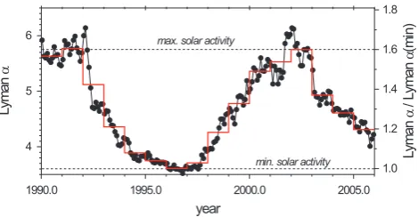
As seen in Fig. 2 the solar activity changes markedly dur-ing the observation period between 1990 and 2005, here characterized by changes in the solar Lyman α radiation (Woods, 2006), which is the most important solar radiation for the ionisation of the ionospheric D-region. The black dots are monthly mean values, the red step-like curve char-acterizes the variation of yearly mean values. The years of maximum solar activity are 1991 and 2002, with the lowest activity observed in 1996.

The influence of the solar activity upon the zonal wind field can be seen in Fig. 3, where during the years of high solar activity (years 1990–1992 and 2000–2002) the winds are markedly stronger than during the period of low solar activity (years 1995–1997). The fact that the winds during the second solar maximum (2000–2002) are stronger than at the first maximum (1990–1992) suggested possible trends.

Both phenomena, the influence of the solar activity on the mesospheric wind field, as well as trends in the wind field,

Fig. 2. Variation of the solar Lyman α radiation (units: 1011ph. cm−2s−1) between 1990–2005 (Woods, 2006). Black dots are monthly mean values, the red curve is based on yearly mean values.

Fig. 3. Mean height-time cross section of the zonal wind for three different time intervals derived from MF-radar data at Juliusruh.

are analysed by the following twofold regression equation

v=a+b·Lyα+c·year. (1) Such regression analyses have been carried out separately for the zonal and meridional prevailing winds, as well as for the amplitude of the semidiurnal tide at heights between about 68 km and 93 km, using monthly median values.

Fig. 4. Mean height-time cross section of the partial regression co-efficientb(see Eq. 1) between the mesospheric zonal wind at Julius-ruh and the solar activity.

Fig. 5. Seasonal variation of the partial regression coefficientb(see Eq. 1) between the mesospheric zonal wind at Juliusruh and the solar activity for different heights (significance levelχmarked by black dots (χ≥95%), grey dots (χ≥90%), and crosses (χ <90%)).

3.1 Solar influence upon the mesospheric wind field The next three subsections deal with the solar influence on the three investigated wind parameters separately, using in Eq. (1) the solar Lymanαvalues as the solar activity index. Due to the strong correlation between the monthly Lymanα

values and F10.7 solar activity indices, the regression results are nearly identical as if the F10.7 values would be used. 3.1.1 Zonal wind

The influence of the solar activity on the zonal wind is shown in Fig. 4 by a height-time cross section derived from the monthly regression coefficientsb. Whereas during the sum-mer months negative values dominate, in winter more posi-tive values have been derived. Therefore, the easterly wind

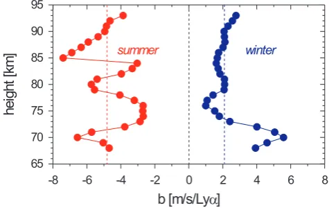
Fig. 6. Partial regression coefficientb(see Eq. 1) between the meso-spheric zonal wind at Juliusruh and the solar activity with a depen-dence on height for summer (red) and winter (blue). Red and blue dashed lines are the corresponding medianbvalues derived from all data.

jet in summer, as well as the westerly wind in winter is en-hanced by increasing solar activity. Due to the intensifica-tion of the summer easterly wind, the region of the easterly wind jet in summer is also extended toward higher altitudes as can also be seen by a comparison of the lower part of Fig. 3 (representing high solar activity) with the middle part of this figure (for low solar activity).

The seasonal variation of the partial regression coefficient

bis shown in Fig. 5 for different altitudes between 70 km and 90 km. Here the significance levelsχ of the individual re-gression coefficients are included withχ≥95% (black dots),

χ≥90% (grey dots), as well as for nonsignificant values with

χ <90% (crosses). The significance levels have been esti-mated with the Fisher’s F test (Taubenheim, 1969). As seen from Fig. 5 the most significant b values were derived for the summer months, whereas in winter only some individual regression coefficients are significant.

In Fig. 6 meanb profiles are presented which have been calculated from the monthly b values for the summer and winter half year (summer: months 4–9, winter: months 10– 3). The dashed vertical lines mark the corresponding me-dian values over all heights (summer:−4.8 m/s/Lyα, winter: 2.1 m/s/Lyα). It has to be mentioned here, thatbvalues are shown for each sampling height (each km), in spite of the fact that the height resolution of the radar measurements is larger, as reported in Sect. 2. In other figures we present, therefore, often only data which are separated by 5 km. Nevertheless, we found in Fig. 6 at all heights negativebvalues in summer and positive values in winter.

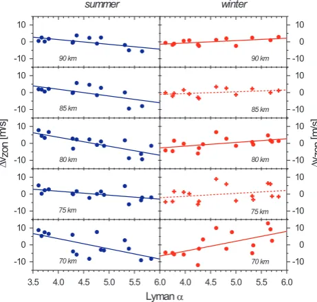
Fig. 7. Dependence of detrended zonal wind values at Juliusruh on solar activity for summer and winter conditions at different heights. Positive relations are red, negative relations blue. Significance lev-els are characterized by full lines and dots (χ≥95%), nonsignificant levels by dashed lines and crosses (χ <90%).

October until March) and linear regressions with a depen-dence on the Lymanαflux have been estimated. The results are presented in Fig. 7 for five different heights. As to be expected, due to the results presented in Figs. 4–6, all re-gressions in summer are negative with a significance level

χ≥95% (full circles and full regression line), whereas in winter all regressions are positive. However, in winter some of the regressions are nonsignificant (χ <90%, crosses with dashed regression lines).

3.1.2 Meridional wind

The impact of the solar activity on the meridional wind com-ponent is presented in Fig. 8 by the seasonal variation of the partial regression coefficientb for five heights between 70 km and 90 km. During most months and heights theb val-ues are positive with larger valval-ues in summer than in winter. Also, the significance level of the regression values is higher in summer. Only during summer were significantb values derived (black dots:χ≥95%; grey dots:χ≥90%). The solar influence in winter is small and nonsignificant.

The results presented in Fig. 8 are confirmed by the anal-yses with detrended data series of the meridional winds us-ing the same method as described above in connection with Fig. 7. The regression lines in Fig. 9 are positive for all heights during summer. In four out of five heights the signif-icance of these regressions is significant withχ≥95% (dots with full regression line). During winter the regression lines are mainly nonsignificant positive or negative; only for the

Fig. 8. Seasonal variation of the partial regression coefficientb (see Eq. 1) between the mesospheric meridional wind at Juliusruh and the solar activity for different heights. Significance levelχis marked by black dots (χ≥95%), grey dots (χ≥90%), and crosses (χ <90%).

Fig. 10. Seasonal variation of the partial regression coefficientb (see Eq. 1) between the amplitude of the semidiurnal tide at Julius-ruh and the solar activity for different heights. Significance levelχ is marked by black dots (χ≥95%), grey dots (χ≥90%), and crosses (χ <90%).

height of 90 km is the regression positive with a significance levelχ≥90%.

3.1.3 Amplitude of semidiurnal tide

The influence of solar activity on the amplitude of the semidiurnal component is very small and in general, non-significant. This can be seen by the seasonal variation of the partial regression coefficient shown in Fig. 10. Here the monthlybvalues are positive (70 km and 80 km) or negative (75 km, 85 km, 90 km), and the corresponding significance levels are in general small. Only in four cases were signif-icant values detected. These results qualitatively agree with the analyses of the detrended data series as shown in Fig. 11. As the monthlybvalues in Fig. 10 do not show any marked seasonal variations, in Fig. 11 only yearly mean values have been used to obtain more significant results. However, only at 75 km a significant negative regression line was derived (χ≥90%).

3.2 Trends in the mesospheric wind field

The next three subsections deal with the analysis of long-term trends in the mesospheric wind field based on Eq. (1). In particular the partial regression coefficientcwill be pre-sented with a dependence on height and season for different characteristic wind parameters.

Fig. 11. Dependence of detrended values of the amplitude of the semidiurnal tide at Juliusruh on solar activity for yearly mean con-ditions at different heights. Positive relations are red, negative rela-tions blue. Significance levels are characterized by dashed lines and dots (χ≥90%), nonsignificant levels by dashed lines and crosses (χ <90%).

Fig. 12. Mean height-time cross section of the trend in the meso-spheric zonal wind at Juliusruh (partial regression coefficientcdue to Eq. 1).

3.2.1 Zonal wind

The trends in the mesospheric zonal wind field are shown by a height-time cross section in Fig. 12, resulting fromc

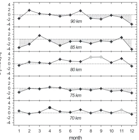
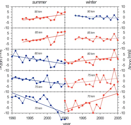
Fig. 13. Seasonal variation of the trend in the mesospheric zonal wind at Juliusruh (partial regression coefficientcdue to Eq. 1) for different heights. The significance levelsχ are marked by black dots (χ≥95%), grey dots (χ≥90%), and crosses (χ <90%).

about 83 km and positive above this height. During winter the trends are not so clear, with positive parts dominating at lower heights and negative parts at higher regions. During spring a negative region also reaches up to above 90 km. The same features can also be seen in Fig. 13, where the seasonal variation of the trend parametercis presented for different heights. Most of the summer months have significant trends (black dots: χ≥95%, gray dots: χ≥90%) with a different sign above and below about 83 km. During winter only a few months have significant trends.

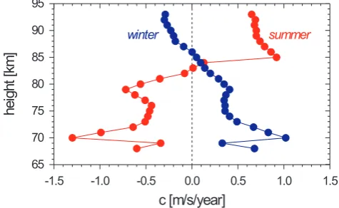
The different behaviour of the trends in summer and win-ter with a dependence on height can very clearly be seen in Fig. 14, where mean profiles are presented calculated from the monthlyc values (summer: from months 4–9, winter: from months 10–3). Here the change in the sign of the trend is near 83 km during summer and near 86 km during winter.

Using zonal wind values after elimination of the solar ac-tivity influence by a similar method, as explained for Fig. 7 in Sect. 3.1.1, linear mean trends for summer and winter have been estimated. The results are presented in Fig. 15 for dif-ferent heights. Whereas during summer all trends shown are significant with χ≥95%, during winter only the trends in two heights are significant (χ≥95% in 70 km and 80 km), whereas the other trends are nonsignificant (χ <90%). The changing sign of the trend with a dependence on height fully agrees with the results presented in Fig. 14.

Fig. 14. Trend of the mesospheric zonal wind at Juliusruh (partial regression coefficientcdue to Eq. 1) with a dependence on height for summer (red) and winter (blue).

3.2.2 Meridional wind

The trends in the meridional component of the mesospheric wind field can be found in Fig. 16 with a dependence on season and height. During summer positive trends have been detected at heights below a transition height near 84 km (detected from trend analyses at every km, not shown here), most of the detected trends are significant (black dots:

χ≥95%). At heights above 84 km the trends become neg-ative, and they are mostly nonsignificant. During winter the monthly trends are positive or negative, but only some of them are significant (black dots: χ≥95%, grey dots:

χ≥90%). The mean seasonal trends derived after elimina-tion of the solar influence are shown in Fig. 17. The derived trends agree in general with the results of Fig. 16. Significant trends were only found in summer at heights below 84 km and during winter only at 90 km.

3.2.3 Amplitude of semidiurnal tide

The seasonal variation of the trends of the semidiurnal tidal amplitude in the mesospheric wind field is presented for dif-ferent heights in Fig. 18. These trends are nearly all positive, their values increase with height, but only some of them are significant. As nearly all trends are positive without marked seasonal variations, only mean yearly trends have been de-rived, combining all 12 months after elimination of the solar activity influence. In Fig. 19 these yearly trends are presented for different heights. All trends are positive and most of them are significant (χ≥95%: 70 km and 80 km;χ≥90%: 85 km and 90 km).

4 Summary and discussion

Fig. 15. Trend of the mesospheric zonal wind at Juliusruh after elimination of the solar activity induced parts for summer and win-ter conditions at different heights. Positive trends are red, negative trends blue. Significance levels are characterized by full lines and dots (χ≥95%), nonsignificant levels by dashed lines and crosses (χ <90%).

Fig. 16. Seasonal variation of the trend in the mesospheric merid-ional wind at Juliusruh (partial regression coefficientcdue to Eq. 1) for different heights. The significance levelsχare marked by black dots (χ≥95%), grey dots (χ≥90%), and crosses (χ <90%).

Due to increasing external noise level (mainly foreign radio transmitters) during night-time conditions the radar

measure-Fig. 17. Trend of the mesospheric meridional wind at Juliusruh after elimination of the solar activity induced parts for summer and win-ter conditions at different heights. Positive trends are red, negative trends blue. Significance levels are characterized by full lines and dots (χ≥95%), nonsignificant levels by dashed lines and crosses (χ <90%).

ments can only successfully be used during 13–16 h around local noon for the derivation of the mesospheric wind field. Therefore, only the semidiurnal tidal component as well as the prevailing zonal and meridional components of the wind field have been derived and used for the investigation of their long-term variations. Due to the limited diurnal measuring time it is impossible to derive the diurnal tidal component with sufficient accuracy.

The available time interval of 16 years with continuous wind observations is not very long for long-term investiga-tions, however, with a duration of about 1.5 solar cycles it seems to be possible to obtain some indications of the so-lar influence and of possible trends. By extension of these observations in the future the accuracy of the derived results may become still more representative. In the presented paper we tried to estimate the significance of the derived results by some statistical tests.

Fig. 18. Seasonal variation of the trend of the semidiurnal tidal amplitude at Juliusruh (partial regression coefficientcdue to Eq. 1) for different heights. The significance levelsχare marked by black dots (χ≥95%), grey dots (χ≥90%), and crosses (χ <90%).

4.1 Influence of the 11-year solar cycle

Due to the results presented in Figs. 4–7 the zonal wind is in-tensified by increasing solar activity, i.e. increasing easterly winds in summer and westerly winds in winter during the whole height range investigated between about 68 km until 93 km. The negative correlation between the summer zonal wind and the solar activity is confirmed by the majority of investigations with other data series (Greisiger et al., 1987; Namboothiri et al., 1993, 1994; Bremer et al., 1997; Jacobi, 1998; Jacobi and K¨urschner, 2006). Only Dartt et al. (1983) and Middleton et al. (2002) reported about a positive correla-tion between summer zonal winds and solar activity. A sim-ilar picture can be found for investigations during the winter season. Here a positive correlation was detected as seen in Figs. 4–7. However the significance level of these correla-tions is slightly smaller than in summer (see Figs. 5 and 7). This positive correlation is confirmed by a lot of other inves-tigations (Sprenger and Schminder, 1969; Dartt et al., 1983; Namboothiri et al., 1993, 1994; Bremer et al., 1997; Jacobi and K¨urschner, 2006). A negative correlation was only de-rived by Greisiger et al. (1987), Merzlyakov and Portnyagin (1999), and Middleton et al. (2002). In conclusion, it can be stated that the solar activity markedly influences the zonal mesospheric wind field. However, the significance level of some investigations (mainly during winter, probably caused by the strong atmospheric variability during this season) is not high enough to obtain final results in each case.

Fig. 19. Trend of the yearly averaged semidiurnal tidal amplitudes at Juliusruh after elimination of the solar activity induced parts for different heights. Significance levels are characterized by full lines and dots (χ≥95%) or dashed lines and dots (χ≥90%), non-significant levels by dashed lines and crosses (χ <90%).

As the meridional wind component is essentially smaller than the zonal component, the derived correlations with solar activity become more uncertain. Due to the results in Figs. 8 and 9 the correlation between the meridional wind and the solar activity is during the summer months mainly positive with a sufficient significance level. During winter the cor-relation becomes smaller and is in general positive, but dur-ing some individual months at different altitudes the correla-tion can be even negative. Therefore, the significance level during winter is mostly below 90%. Other authors found similar results for summer (Dartt et al., 1983; Jacobi, 1998; Merzlyakov and Portnyagin, 1999) and winter (Sprenger and Schminder, 1969; Bremer et al., 1997; Jacobi, 1998; Jacobi and K¨urschner, 2006). But there are also some authors who found opposite results or no correlations.

wind observations which are only seldom available. Such long data series are necessary to separate the solar activity-induced part from the trend, which is normally assumed to be linear. But also other trend types can be used (e.g. parabolic trends, as derived by Portnyagin et al., 2006). Long-term trends have been derived mostly from data series at altitudes between 90–95 km, often from radar meteor observations without interferometric height estimations. Also, some old LF wind measurements have been made without exact height estimations (Sprenger and Schminder, 1969). Therefore, the comparison of the trend results presented in Sect. 3.2 with other results can only be made for heights near 90 km.

Due to the results shown in Figs. 12–15, the trends in the zonal wind field are different with a dependence on height and season. During summer the trends are negative below about 83 km and positive above this altitude, in both cases, with significance levels between 90–95%. During winter the behaviour of the trends is nearly opposite, with positive trends below about the 86 km height and negative above this altitude. The significance levels are smaller than in summer, however, for some selected heights and months, up to 95%. Some publications qualitatively confirm our results for the summer months (Jacobi, 1998; Jacobi and K¨urschner, 2006; Portnyagin et al., 2006) and the winter months (Portnyagin et al., 1993; Bremer et al., 1997; Merzlyakov and Portnyagin, 1999). However, in some other papers trends with different signs are reported, for example, for summer (Portnyagin et al., 1993; Bremer et al., 1997; Merzlyakov and Portnyagin, 1999) and for winter (Jacobi and K¨urschner, 2006). In some papers results of different stations are presented with partly different signs (Jacobi et al., 2005). In the paper by Port-nyagin et al. (2006) different trends have been derived for two subintervals divided by a break point. For comparison with our trends only the trends of the last interval are used, as this time interval agrees better with the interval investi-gated in this paper. Also in these publications (Jacobi et al., 2005; Portnyagin et al., 2006), the signs of the trends of dif-ferent measurements are partly difdif-ferent. A qualitative agree-ment of the zonal wind trend profiles in Fig. 14 can be found by a comparison with model results derived by Schmidt et al. (2006), using the Hamburg Model of the Neutral and Ion-ized Atmosphere (HAMMONIA). From the global results presented in their Fig. 11 the difference of the zonal wind field for doubled CO2 conditions and normal CO2 content

1vzon=vzon(2CO2)−vzon(CO2)has been extracted for a

lati-tude of 55◦N. These results presented in Fig. 20 show

qual-Portnygin, 1999; Jacobi et al., 2003, 2005; Jacobi and K¨urschner, 2006; Portnygin et al., 2006), however, for heights between about 90–95 km. During winter the trends are only near 70 km positive and at higher altitudes negative (see Fig. 17). The only significant trend has been derived at 90 km in qualitative agreement with other results (Jacobi and K¨urschner, 2006; Portnyagin et al., 2006).

Fig. 20. Changes in the zonal wind at 55◦N due to doubling of the atmospheric CO2content with a dependence on height estimated

from model results with HAMMONIA (Schmidt et al., 2006) for summer (red) and winter conditions (blue).

4.3 General remarks

Mesospheric long-term wind observations have been carried out until now only at a few stations worldwide. There-fore, the number of available data series is relatively small. Furthermore, different measuring techniques and evaluation methods have been used. Also, the analysed heights and the observation periods are often different. Therefore, many of the detected differences of the solar activity-induced varia-tions and of the derived trends may be caused by such tech-nical details. To a certain extent the available time interval is also insufficient to separate the solar influence and a possi-ble long-term trend. Therefore, in the two subsections above only the sign of the different solar forced regression coeffi-cients, as well as trend values have been compared and not their absolute values.

5 Conclusions

Based on MF-radar observations at Juliusruh between 1990 and 2005 the solar-induced influences on the mesospheric wind field, as well as linear long-term trends of different wind parameters have been derived by a twofold regression analysis. The main results can be summarized as follows:

– Increasing solar activity amplifies the mesospheric wind field by an enhancement of the easterly winds in sum-mer (significant connection) and of the westerly winds in winter (only partly significant).

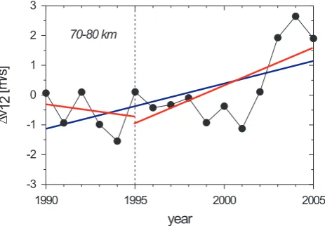
Fig. 21. Trends of the yearly averaged semidiurnal tidal amplitudes at Juliusruh for the height interval 70–80 km after elimination of the solar induced parts derived for the full observation period from 1990 until 2005 (blue line) and for the two subintervals before and after 1995 (red lines).

– The meridional wind is positively connected with the solar activity with higher significance levels during summer months than in winter.

– The influence of the solar activity on the semidiurnal tidal amplitude is small and nonsignificant.

– The trends in the zonal wind component are different in dependence on height, negative below 83 km in summer and positive above this height. During winter an oppo-site behaviour occurs with positive trends above 86 km and negative values below this height. The significance levels of the trends in summer are better than in win-ter. The trends qualitatively agree with model results (Schmidt et al., 2006).

– The significance values of the trends in the meridional wind are smaller than in the zonal wind. Significant trends have been detected in summer only below 85 km and in winter only at 90 km.

– The trends in the amplitude of the semidiurnal tidal component are positive, at most heights even signifi-cant, if yearly mean values have been used. The pos-itive trend may be caused by an increasing ozone trend since about 1995 above Central Europe (Krzyscin et al., 2005).

– To enhance the significance level of the derived long-term variations (solar influence, as well as trends) it is necessary to extent the data series of mesospheric wind components by further observations in the future with-out essential changes in the technique and the evaluation method.

Acknowledgements. Topical Editor U.-P. Hoppe thanks J.

Terr. Phys., 64, 805–816, 2002.

Bremer, J., Schminder, R., Greisiger, K.M., Hoffmann, P., K¨urschner, D., and Singer, W.: Solar cycle dependence and long-term trends in the wind field of the mesosphere/lower thermo-sphere, J. Atmos. Solar-Terr. Phys., 59, 497–509, 1997. Dartt, D., Nastrom, G., and Belmont, A.: Seasonal and solar cycle

wind variations, 80–100 km, J. Atmos. Terr. Phys., 45, 707–718, 1983.

D’yachenko, V. A., Lysenko, I. A., and Portnyagin, Yu. I.: Long term periodicities in lower thermospheric wind variations, J. At-mos. Terr. Phys., 48, 1117–1119, 1986.

Fraser, G. J.: Long-term variations in mid-latitude southern hemi-sphere mesospheric winds, Adv. Space Res., 10, 247–250, 1990. Fraser, G. J., Portnyagin, Yu. I, Forbes, J. M., Vincent, R. A., Ly-senko, I. A., and Makarov, N. A.: Diurnal tide in the Antarctic and Arctic mesosphere/lower thermosphere regions, J. Atmos. Terr. Phys., 57, 383–393, 1995.

Greisiger, K. M., Schminder, R., and K¨urschner, D.: Long-period variations of wind parameters in the mesopause region and the solar cycle dependence, J. Atmos. Terr. Phys., 49, 281–285, 1987.

Hoffmann, P., Singer, W., Keuer, D., Schminder, R., and K¨urschner, D.: Partial reflection drift measurements in the lower ionosphere over Juliusruh during winter and spring 1989 and comparison with other wind observations, Z. f. Meteorol., 40, 405–412, 1990. Jacobi, Ch.: On the solar cycle dependence of winds and planetary waves as seen from mid-latitude D1 LF mesopause region wind measurements, Ann. Geophys., 16, 1534–1543, 1998,

http://www.ann-geophys.net/16/1534/1998/.

Jacobi, Ch. and K¨urschner, D.: Long-term trends of the MLT re-gion winds over Central Europe, Phys. Chem. Earth, 31, 16–21, doi:10.1016/j.pce.2005.01.004, 2006.

Jacobi, Ch., Lange, M., and K¨urschner, D.: Influence of anthro-pogenic climate gas changes on the summer mesospheric/lower thermospheric meridional wind. Meteorol. Zeitschr., 12, 37–42, doi:10.1127/0941/2003/0012-0037, 2003.

Jacobi, Ch., Portnyagin, Yu. I., Merzlyakov, E. G., Solovjova, T. V., Makarov, N. A., and K¨urschner, D.: A long-term com-parison of mesopause region measurements over Eastern and Central Europe, J. Atmos. Solar-Terr. Phys., 67, 229–240, doi:10.1016/j.jastp.2004.10.002, 2005.

Jacobi, Ch., Schminder, R., K¨urschner, D., Bremer, J., Greisiger, K. M., Hoffmann, P., and Singer, W.: Long-term trends in the mesopause wind field obtained from LF D1 wind measurements at Collm, Germany, Adv. Space Res., 20, 11, 2085–2088, 1997. Krzyscin, J. W., Jaroslawski, J., and Rajewska-Wiech, B.:

Begin-ning of the ozone recovery over Europe? – Analysis of the total ozone data from ground-based stations, 1964–2004, Ann. Geo-phys., 23, 1685–1695, 2005,

http://www.ann-geophys.net/23/1685/2005/.

Phys., 55, 1325–1334, 1993.

Namboothiri, S. P., Meek, C. E., and Manson, A. H.: Variations of mean winds and solar tides in the mesosphere and lower thermo-sphere over time scales ranging from 6 months to 11 yr: Saska-toon, 52◦N, 107◦W, J. Atmos. Terr. Phys., 56, 1313–1325, 1994. Portnyagin, Yu. I., Merzlyakov, E. G., Solovjova, T. V., Jacobi, Ch., K¨urschner, D., Manson, A., and Meek, C:: Long-term trends and year-to-year variability of mid-latitude mesosphere/lower ther-mosphere winds, J. Atmos. Solar-Terr. Phys., 68, 1890–1901, doi:10.1016/j.jastp.2006.04.004, 2006.

Portnyagin, Yu. I., Forbes, J. M., Fraser, G. J., Vincent, R. A., Av-ery, S. K., Lysenko, I. A., and Makarov, N. A.: Dynamics of the Antarctic and Arctic mesosphere and lower thermosphere re-gions – I. The prevailing wind, J. Atmos. Terr. Phys., 55, 827– 841, 1993.

Randel, J. W., Wu, F., V¨omel, H., Nedoluha, G. E., and Forster, P.: Decreases in stratospheric water vapor after 2001: Links to changes in the tropical tropopause and the Brewer-Dobson circulation, J. Geophys. Res., 111, D12312, doi:10.1029/2005JD006744, 2006.

Ross, M. N. and Walterscheid, R. L.: Changes in the solar forced tides caused by stratospheric ozone depletion, Geophys. Res. Lett., 18, 420–423, 1991.

Schmidt, H., Brasseur, G. P., Charron, M., Manzini, E., Giorgetta, M. A., Diehl, T., Fomichev, V. I., Kinnison, D., Marsh, D., and Walters, S.: The HAMMONIA chemistry climate model: Sensi-tivity of the mesopause region to the 11-year solar cycle and CO2

doubling, J. Climate, 19, 3903–3931, 2006.

Schminder, R., K¨urschner, D., Singer, W., Hoffmann, P., Keuer, D., and Bremer, J.: Representative height-time cross-sections of the upper atmosphere wind field over Central Europe 1990–1996, J. Atmos. Solar-Terr. Phys., 59, 2177–2184, 1997.

Singer, W., Latteck, R., Holdsworth, D., and Kristiansen, T.: A new narrow beam MF radar at 3 MHz for studies of the high-latitude middle atmosphere: System description and first results, Proc. of the Tenth Workshop on Techn. and Scientific Aspects of MST Radar (MST10), 385–390, 2003.

Singer, W., Hoffmann, P., Keuer, D., Schminder, R., and K¨urschner, D.: Wind in the middle atmosphere with partial reflection mea-surements during winter and spring in middle Europe, Adv. Space Res., 12(10), 299–302, 1992.

Sprenger, K. and Schminder, R.: Solar cycle dependence of winds in the lower ionosphere, J. Atmos. Terr. Phys., 31, 217–221, 1969.

Taubenheim, J.: Statistische Auswertung geophysikalischer und meteorologischer Daten, Akademische Verlagsgesellschaft Geest und Portig K.-G., Leipzig, 1969.