6.1
Chapter
VII
Non Parametric Test
...
Purpose of
Chapter
Nonparametric statistics or
distribution-free tests are those
that do not rely on parameter
estimates or precise assumptions
about the distributions of
variables.
7.1 Introduction
Note: Parametric tests assume that the data follows a particular distribution e.g for t-tests, ANOVA and regression, the data needs to be normally distributed. Parametric tests are more powerful than non-parametric tests, when the assumptions about the distribution of the data are true. This means that they are more likely to detect true differences or relationships that exist.
Parametric vs Nonparametric Statistics
• Parametric Statistics are statistical techniques based on assumptions about the population from which the sample data are collected.
– Assumption that data being analyzed are randomly selected from a normally distributed population.
– Requires quantitative measurements that yield interval or ratio level data.
• Nonparametric Statistics are based on fewer assumptions about the population and the parameters. – A variety of nonparametric statistics are available for use with nominal data, ordinal and even
quantitative (convert to ordinal)
– When the data is quantitative but does not meet the assumptions of normality and Homogeneity, in the case of more than two groups.
Nonparametric statistics (or tests) based on the ranks of measurements are called rank statistics (or rank tests).
Analysis for Non Parametric Tests according to the number of samples and type of variable
Advantages and Disadvantages of non-parametric test
Advantages Disadvantages
Can be used when nothing known about population
– Therefore can’t break or violate crucial assumptions for confidence interval and
Less powerful even with same sample size
hypothesis tests
Used with all scales. Can use nominal or ordinal data compared to interval or ratio data
– Nominal = names or labels, Eg. Gender (males, females)
Ordinal = imply some order or rank, Eg. Grade of study
Can be used with smaller samples
The computations on nonparametric statistics are usually less complicated than those for parametric statistics, particularly for small samples.
Less efficient
Nonparametric tests can be wasteful of data if parametric tests are available for use with the data
Nonparametric tests are usually not as widely available and well know as parametric tests
For large samples, the calculations for many nonparametric statistics can be tedious
7.2 Chi Square Independent Test (c2) (Contingency Table Analysis)
A chi square (c2) statistic is used to investigate whether distributions of categorical variables differ from one another. Basically categorical variable yield data in the categories and numerical variables yield data in numerical form. Responses to such questions as "What is your major?" or do you own a car?" are categorical because they yield data such as "Business" or "no". In contrast, responses to such questions as "How tall are you?" it is numerical. Numerical data can be either discrete or continuous. The table below may help you see the differences between these two variables.
Data Type Question Type
Possible Responses
Categorical What is your sex? male or female
Numerical – Discrete How many children do you have? 0 or 1 or 2 or…
Numerical - Continuous How tall are you? 72 inches
A test of independence assesses whether paired observations on two variables, expressed in a contingency table, are independent of each other (e.g. polling responses from people of different nationalities to see if one's nationality affects the response).
Important note: The data are assumed to be a random sample. The expected frequencies for each category should be at least 1. No more than 20% of the categories should have expected frequencies of less than 5."
Steps in Hypothesis Testing
1. Formulate the appropriate null and alternative hypothesis Ho: There is no relationship between variables
Ha: There is a relationship between the variables 2. Specify the desired level of significance (a)
a , (level of significance); typical values are .01, .05, or .10 3. Computing the Test Statistic
Calculate the chi-squared test across all the categories. Oij = observed frequency
eij = expected frequency
Look at the Sig. Or P_ value, if this value is less than the significance level (α = .05) we reject Ho.
Example 1
An on-line music service company wants to know (for the purposes of designing a marketing campaign) if customer age is important in deciding to subscribe, and, if so, which age groups are most likely to subscribe to its services. The company has gathered a random sample of 1000 people from the population, and asked each person whether he or she would subscribe to the service. The company knows which age group the person falls into: under 21 years of age, 21 - 34 years of age, and 35 years or older. The data is presented in the following table:
Table 7.1. Decision to purchase the services by customer’s age Decision to
purchase the
services Under 21 21-34
35 and
over Total
Yes 120 262 237 619
No 41 103 237 381
Total 161 365 474 1000
Solution:
Step 1: Hypothesis
Ho: There is no relationship between the customer age groups and to make a decision to purchase the services.
Ha: There is a relationship between the customer age groups and to make a decision to purchase the services.
Step 2: Level of significance: α = 0.05
Step 3: Computing the Test Statistic
Compares observed frequencies within groups with their expected frequencies
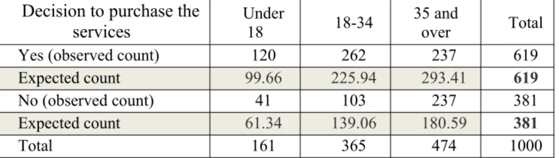
In the following table we observe the expected values for each observed value.
Decision to purchase the
services Under18 18-34
35 and
over Total
Yes (observed count) 120 262 237 619
Expected count 99.66 225.94 293.41 619
No (observed count) 41 103 237 381
Expected count 61.34 139.06 180.59 381
Total 161 365 474 1000
To calculate the chi-square statistic, take the difference between the Observed Count and the Expected Count, square the difference, and divide by the Expected Count, producing the following solution:
Sig=.000 is less than .05, so we reject null hypothesis, and conclude at 5% of level of significance that the age groups differ in their decision to purchase the service, in the other hand there is a relationship
between the age of the customer and to make a decision to purchase the services.
Step to pass the data to SPSS when we have contingence tables
For SPSS to successfully analyze this problem, enter the two variables “decision to purchase the services (service)” and “Customer Age (age)” as integer variables (no decimals). In the “decision” row (we’re still in the “Variable View” tab), click the cell in the “Values” column, as shown in the following figure. Decision to purchase:
Code Observation
1 Yes
2 No
Create the same for the second variable (for the variable in Column) Age:
Code Observation
1 Under 18
2 18 - 34
3 35 and over
Finally enter the data in (Data view), as noted in the following table
Code for Decision
Code for
Age Frequency
1 1 120
1 2 262
1 3 237
2 1 41
2 2 103
2 3 237
Finally, let’s perform the Chi Square:
Analyze < Descriptive Statistics < Crosstab < and follow the step that we show in the picture:
Output
Decision * Age Crosstabulation
Age
Total Under 18 18 - 34 35 andover
Decision Yes 120 262 237 619
No 41 103 237 381
Total 161 365 474 1000
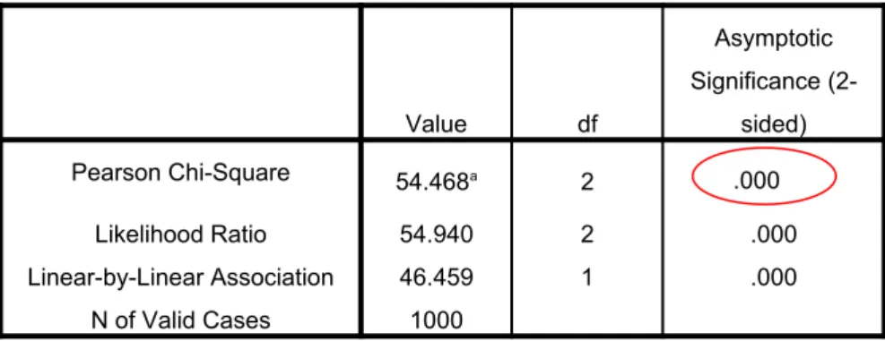
Value df
Asymptotic
Significance (2-sided)
Pearson Chi-Square 54.468a 2
Likelihood Ratio 54.940 2 .000
Linear-by-Linear Association 46.459 1 .000 N of Valid Cases 1000
Making decision and interpret result: Since Sig. = .000 < .05, we can reject null hypothesis, In other words, there is a relationship between the age of the customer and to make a decision to purchase the services (So we reject the null hypothesis and conclude that the age groups differ in their decision to
purchase the service).
Example 2.
In a sample of 103 people aged 25 to 50 years want to determine whether cough in the morning is associated with cigarette smoking.
Table 7.2. Smoke cigarettes and cough at morning Do you cough at
morning?
Do you smoke cigarettes?
Total
Yes No
Yes 45 24 69
No 15 19 34
Total 60 43 103
Step 1: Hypothesis
Ho: Coughing in the morning is independent of cigarette smoking Ha: Coughing in the morning is associated with cigarette smoking
Step 2: Level of significance: α = 0.05
Step 3: Computing the Test Statistic ꭓ2
= 4.17
Step 4: Making a decision and interpreting the result: The calculate c2 = 4.17, and Sig or p_value =
0.041. is less than .05, so we reject null hypothesis. At 5% of level of significance cough at morning is associated with cigarette smoking.
Example 3: Use the data of file that has the SPSS "demo.sav"
This is a hypothetical data file that concerns a purchased customer database, for the purpose of mailing monthly offers. Whether or not the customer responded to the offer is recorded, along with various demographic information.
Crosstabulation tables (contingency tables) display the relationship between two or more categorical (nominal or ordinal) variables. The size of the table is determined by the number of distinct values for each variable, with each cell in the table representing a unique combination of values. Numerous statistical tests are available to determine whether there is a relationship between the variables in a table. Step in SPSS:
Analyze < Descriptive Statistics < Crosstab < and follow the step that we show in the picture
Interpretation Results:
What factors affect the products that people buy?
The most obvious is probably how much money people have to spend. In this example we’ll examine the relationship between income level and PDA (personal digital assistant) ownership.
Descriptive interpretation:
The cells of the table show the count or number of cases for each joint combination of values. For example,
455 people in the income range $25,000 – $49,000 had own PDAs.
None of the numbers in this table, however, stand out in an obvious way, indicating any obvious relationship between the variables.
It is often difficult to analyze a cross tabulation simply by looking at the simple counts in each cell
Inferential interpretation:
Significance Testing for Crosstabulations
A number of tests are available to determine if the relationship between two crosstabulated variables is significant. One of the more common tests is Chi-square. One of the advantages of chi-square is that it is appropriate for almost any kind of data.
Pearson chi-square tests the hypothesis that the row and column variables are independent.
1. Hypothesis
Ho: The variables Income and Owns PDA are independent. Ha: The variables Income and Owns PDA are related. 2. Level of significance α = .05
3.Test Statistic: c2 = 37.677, Sig = .000
Output from SPSS
Chi-Square Tests
Value df Asymp. Sig.(2-sided) Pearson Chi-Square 37.677a 3 .000
Likelihood Ratio 37.313 3 .000 Linear-by-Linear
Association 36.537 1 .000 N of Valid Cases 6400
a. 0 cells (0.0%) have expected count less than 5. The minimum expected count is 228.73.
4. Making a Decision and Interpreting the Result: since the Sig = .000 < .05, so we can to reject Ho. At the level of significance of 5% the variables Income and Owns PDA are related.
Interpretation: the percentage of people who had own PDAs rises as the income category rises.
Differences between independent groups 7.3 Mann-Whitney U-Test (or ranked-sum)
"salary" and your independent variable would be "educational level", which has two groups: "high school" and "university"). The Mann-Whitney U test is often considered the nonparametric alternative to the independent t-test although this is not always the case.
Nonparametric counterpart of the t test for independent samples • Does not require normally distributed populations
• May be applied to ordinal data
• Actual measurements not used – ranks of the measurements used
Assumptions
– Independent Samples – At Least Ordinal Data
Steps in Hypothesis Testing
1. Formulate the appropriate null and alternative hypothesis Ho: Both groups are the same (there is no difference) Ha: Both groups are not the same
2. Specify the desired level of significance (a)
a , (level of significance); typical values are .01, .05, or .10 3. Computing the Test Statistic
4. Making a decision and interpreting the result of the test
Reject Null Hypothesis if sig is less or equal than .05 (significant result) Don’t Reject Null Hypothesis if sig is more than .05 (non-significant result)
Example 1
Is this sufficient evidence to indicate a difference in the average height of the groups? The data is in the following table 5.3:
Heights of males (cm) 193 188 185 183 180 178 170 Heights of females (cm) 175 173 168 165 163
Solution
Ho: Male and female students are the same height (the distribution of heights for the two groups are
equal)
Ha: Male and female students are not the same height (the distribution of heights for the two groups are
not equal)
Mann-Whitney U Rank Sum Test – Solution in SPSS
Solution
Example 2
Decision: Sig .010 <.05 Reject Null Hypothesis at α= .05
Consider the following data of the number of minutes needed by two groups of factory workers to learn to assemble a chain saw. Group A received classroom training, whereas Group B received only on –the-job- training.
Group A 35 39 51 63 48 31 29 41 55
Group B 85 28 42 37 61 54 36 57
We wish to decide whether the difference between the means is significant. Output from SPSS
Ranks
Group N Mean Rank Sum of Ranks
Time A 9 8.22 74.00
B 8 9.88 79.00
Total 17
Test Statisticsa
Time
Mann-Whitney U 29
Wilcoxon W 74
Z -0.674
Asymp. Sig. (2-tailed) 0.501 Exact Sig. [2*(1-tailed
Sig.)] .541b
a. Grouping Variable: Group b. Not corrected for ties. Since U1 = 43, U2 = 29
U2 <U1, then U=29
Uc= 29 > Ucritical = 15,
Making a Decision and Interpreting the Result: Since Sig is more than .05, we do not reject the null hypothesis, at level of significance α=0.05, therefore is not significant differences between the means of these two groups.
Differences between dependent or related groups (Matched-Pairs)
Parametric Nonparametric
Compare two variables measured in the same sample
t-test for dependent samples
Sign test
Wilcoxon’s matched pairs test or Mc Nemar If more than two variables are
measured in same sample Repeated measures ANOVA Friedman’s two way analysis of variance
7.4 Wilcoxon Rank
The Wilcoxon Rank Test is a non-parametric statistical hypothesis test, used when comparing two related samples, matched samples, or repeated measurements on a single sample to assess whether their population mean ranks differ (i.e. it is a paried difference test). It can be used as an alternative to the paried Student’s t-test (before and after studies), Studies in which measures are taken on the same person or object under different conditions, studies of twins or other relatives or the t-test for dependent samples when the population cannot be assumed to be normally distributed.
Random Samples
Populations are continuous
Can Use Normal Approximation If ni ≥15 Steps in Hypothesis Testing
1. Formulate the appropriate null and alternative hypothesis
H0: both samples come from the same underlying distribution (there is no difference)
Ha: both samples are not come from the same underlying distribution
2. Specify the desired level of significance (a)
a , (level of significance); typical values are .01, .05, or .10 3. Determine the Critical value
Wilcoxon Rank Sum - Table (Portion)
Selected Critical Values of the Wilcoxon Statistics (T) for alpha = .1 and .05
Number of Pairs
Alpha Level
0.1 0.05
5 0
6 2 0
7 3 2
8 5 3
9 8 5
10 10 8
12 17 13
15 30 25
20 60 52
25 100 89
Note: T is significant at the chosen alpha level if is smaller than the critical value given in the table
4. Computing the Test Statistic: Where:
T is the sum of the less ranks when you compare the positive and negative sign n is the number of matched pairs
Procedure:
1. Obtain Difference Scores (D=X1 – X2) are calculated and then ranked ignoring the
sign of the difference (table 5.3). Notice that where there are tied values of the differences, we have allocated the average of the ranks which would be given if it were possible to separate the score. Take care: Zero differences are ignored and are not ranked.
2. The ranks of the differences can now have the sign of the difference reattached. 3. The positive or negative sign is assigned to each rank score, and the scores for the
positive or negative groups are separately totaled.
4. Sum the Ranks separately, (T+ and T- ), and “T = T is the smaller sum of ranks”
5. Making a decision and interpreting the result of the test
Reject Null Hypothesis if your calculated value of T is equal to or less than the critical value; Tc≤ Tcritical (significant result).
Don’t Reject Null Hypothesis if your calculated value is greater than the critical value; Tc >
Tcritical (non-significant result)
Calculate Wilcoxon Rank:
• n is the number of matched pairs
• If n > 15, T is approximately normally distributed, and a Z test is used.
• If n ≤ 15, a special “small sample” procedure is followed in the next example.
Example
The mayor of a city wants to see if pollution levels are reduced by closing the streets to the car traffic. This is measured by the rate of pollution every 60 minutes (8am - 22pm: total of 15 measurements) in a day when traffic is open, and in a day of closure to traffic, the data of air pollution is in the following table 5.5:
Table 5.5. Rate of pollution in different situation
With traffic: 214 159 169 202 103 119 200 109 132 142 194 104 219 119 234
Without
traffic: 159 135 141 101 102 168 62 167 174 159 66 118 181 171 112
It is clear that the two groups are paired, because there is a bond between the readings, consisting in the fact that we are considering the same city (with its peculiarities weather, ventilation, etc.) albeit in two different days. Not being able to assume a Gaussian distribution for the values recorded, we must proceed with a non-parametric test, the Wilcoxon signed rank test.
Solution:
H0: both samples come from the same underlying distribution
Ha: both samples are not come from the same underlying distribution
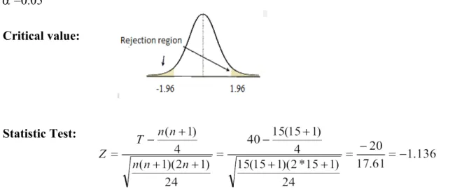
n = 15 a =0.05
Critical value:
Statistic Test:
Making a Decision and Interpreting the Result of the Test
Sig = .256, we cannot reject the null hypothesis Ho of equality of the means.
Therefore the closing roads to traffic did not bring any improvement in terms of rate of pollution.
Wilcoxon Report in SPSS
Ranks Test Statisticsa
N
Mean Rank
Sum of Ranks
Without_traffic -With_traffic
Without_traff ic -With_traffic
Negative Ranks
9a 8.89 80
Z -1.136b
Positive
Ranks 6
b 6.67 40 Asymp. Sig.
(2-tailed) 0.256
Ties 0c a. Wilcoxon Signed Ranks Test
Total 15 b. Based on positive ranks.
a. Without_traffic < With_traffic b. Without_traffic > With_traffic c. Without_traffic = With_traffic
Making a Decision and Interpreting the Result of the Test from result of statistic software SPSS
Since Sig.=0.256>0.05, we can’t reject the null hypothesis, at α=0.05. There is No evidence for unequal distribution. Therefore the closing roads to traffic did not bring any improvement in terms of rate of pollution.
Nonparametric Tests for Multiple Independent Samples
The nonparametric tests for multiple independent samples are useful for determining whether or not the values of a particular variable differ between two or more groups. This is especially true when the assumptions of ANOVA are not met.
The Kruskal-Wallis test is a one-way analysis of variance by ranks. It tests the null hypothesis that multiple independent samples come from the same population. Unlike standard ANOVA, it does not assume normality, and it can be used to test ordinal variables.
7.5 Kruskal-Wallis H
When a researcher wishes to compare three or more groups or populations and the data are ordinal, the Kruskal-Wallis test is the appropriate statistical technique, or when the data is numerical but the assumptions does not have to assume that the underlying populations are normally distributed or the equal variances.
It is used to test the null hypothesis that all populations have identical distribution functions against the alternative hypothesis that at least two of the samples differ only with respect to location (median), if at all.
For example, you could use a Kruskal-Wallis H test to understand whether exam performance, measured on a continuous scale from 0-100, differed based on test anxiety levels (i.e., your dependent variable would be "exam performance" and your independent variable would be "test anxiety level", which has three independent groups: students with "low", "medium" and "high" test anxiety levels). Alternately, you could use the Kruskal-Wallis H test to understand whether attitudes towards pay discrimination, where attitudes are measured on an ordinal scale, differed based on job position (i.e., your dependent variable would be "attitudes towards pay discrimination", measured on a 5-point scale from "strongly agree" to "strongly disagree", and your independent variable would be "job description", which has three independent groups: "shop floor", "middle management" and "boardroom").
Data types that can be analyzed with Kruskal-Wallis H
The data points must be independent from each other
the distributions do not have to be normal and the variances do not have to be equal you should ideally have more than five data points per sample
all individuals must be selected at random from the population all individuals must have equal chance of being selected
sample sizes should be as equal as possible but some differences are allowed
Steps in Hypothesis Testing
1. Formulate the appropriate null and alternative hypothesis Ho: Identical Distribution
Ha: At Least 2 Differ
2. Specify the desired level of significance (a)
a , (level of significance); typical values are .01, .05, or .10 3. Determine the Critical Region
df = (r - 1) (c – 1), where “r” is the number of rows and “c” is the number of columns 4. Computing the Test Statistic
Procedure
1. Assign Ranks, Ri , to the n Combined Observations
Smallest Value = 1; Largest Value = n
Average Ties
2. Sum Ranks for Each Group 3. Compute Test Statistic
The H-statistic is calculated as follows:
Where:
Ri = Sum of the ranks of the ith group
ni = Sample size of the ith group
n = Combined sample sizes of all groups
5. Making a decision and interpreting the result of the test: If Hc < than the critical value; do not reject
null hypothesis at α=0.05
Example
An advertising agency employs three different film production companies to produce its television commercials. The advertising agency has taken a sample of five commercials from each of the population houses, and agency executives have ranked the production quality of the commercials from best quality (1) to lowest quality (15). These ranks are show in the next table. Notice that the advertising agency considered two commercials to be ranked of equal quality. Hence, rather than being ranked 3 and 4, the two commercials are each ranked 3.5. The data is in the following Table 6.6.
Solution
Ho: Identical Distribution Ha: At Least 2 Differ α = .05
df = p - 1 = 3 - 1 = 2 Critical Value: Test Statistic: 665 . 0 48 3 . 973 * 05 . 0 ) 1 15 ( 3 5 46 5 5 . 34 5 5 . 39 ) 1 15 ( 15 12 ) 1 ( 3 ) 1 ( 12 2 2 2 2
H H n n R n n H i iTable 7.6. Ranked of the quality of commercials production
Production company
1
Production company
2
Production company
3
9 6 1
5 13 7
3.5 10 15
14 2 12
8 3.5 11
R1=39.5 R2=34.5 R3=46
Making a Decision and Interpreting the Result: If H=0.665 < than the critical value=5.99; we cannot reject null hypothesis at α=0.05, there is no evidence population distribution are different.
Note: When the sample size (ni) from each group or population exceeds 4, H is approximately the same
as χ2 with degree of freedom is (3-1) =2. Table χ2 at the level .05 with two degrees of freedom is 5.991.
Since the calculated H-valued is 0.665, we cannot reject the null hypothesis.
Example with SPSS
Agricultural researchers are studying the effect of mulch color on the taste of crops. Strawberries grown in red, blue, and black mulch were rated by taste-testers on an ordinal scale of one to five (far below to far above average). The results are collected in the following table. Use the Kruskal-Wallis test to determine if taste varies by mulch color.
Customer Taste Color Customer Taste Color
1 1 1 13 3 1
2 3 2 14 4 2
3 2 3 15 5 3
4 1 1 16 4 1
5 2 2 17 3 2
6 4 3 18 3 3
7 2 1 19 3 1
8 4 2 20 3 2
9 4 3 21 3 3
10 2 1 22 2 1
11 4 2 23 3 2
12 3 3 24 5 3
The Kruskal-Wallis test uses ranks of the original values and not the values themselves. That's appropriate in this case, because the scale used by the taste-testers is ordinal.
First, each case is ranked without regard to group membership. Cases tied on a particular value receive the average rank for that value. After ranking the cases, the ranks are summed within groups.
The Kruskal-Wallis statistic measures how much the group ranks differ from the average rank of all groups.
Ranks
Color N MeanRank Taste Red 8 7.69
Blue 8 13.94 Black 8 15.88 Total 24
The degrees of freedom for the chi-square statistic are equal to the number of groups minus one.
Making a Decision and Interpreting the Result: If H = 6.347 > than the critical value = .042; then Reject null hypothesis, at α = 0.05 there is evidence population distribution are different. In other words, the color of the mulch influences the flavor of the strawberries (the black mulch has higher rank)
Nonparametric Tests for Multiple Related Samples
The nonparametric tests for multiple related samples are useful alternatives to a repeated measures analysis of variance. They are especially appropriate for small samples and can be used with nominal or ordinal test variables.
The Friedman procedure tests the null hypothesis that multiple ordinal responses come from the same population. As with the Wilcoxon test for two related samples, the data may come from repeated measures of a single sample or from the same measure from multiple matched samples.
The Cochran Q procedure tests the null hypothesis that multiple related proportions are the same. The Cochran test is a multivariate extension of the McNemar test used for two related samples.
7.6 Friedman Fr -Test
The Friedman’s test is the nonparametric test equivalent to the repeated measures ANOVA, and an extension of the Wilcoxon test.
– it allows the comparison of more than two dependent groups (two or more conditions)
Steps in Hypothesis Testing
1. Formulate the appropriate null and alternative hypothesis Ho: There are no differences between the groups.
Ha: There are differences between the groups.
2. Specify the desired level of significance (a)
a , (level of significance); typical values are .01, .05, or .10 3. Determine the Critical Region
Test Statisticsa,b
Taste Chi-Square 6.347 df 2 Asymp. Sig. .042
Critical value depend how is level of significance (α) and how much is degree of freedom (df) 4. Computing the Test Statistic
Procedure
1. Assign Ranks, Ri = 1 – p, to the p treatments in each of the b blocks
Smallest Value = 1; Largest Value = p
Average Ties
2. Sum Ranks for Each Treatment 3. Compute Test Statistic
Where:
Ri = Sum of the ranks of the ith group
p = Number of treatment b = Number of block
4. Making a Decision and Interpreting the Result: Compare the value of Friedman (Fr) with the tables
of critical values χ2 of Pearson Chi-square
If the value Fr > χ2 we reject null hypothesis
Example
Three new traps were tested to compare their ability to trap mosquitoes. Each of the traps, A, B, and C were placed side-by-side at each five different locations. The number of mosquitoes in each trap was recorded. At the .05 level, is there a difference in the distribution of number of mosquitoes caught by the three traps?
Trap A Trap B Trap C
3 5 0
23 17 15
11 5 7
8 4 2
19 11 5
Solution
Ho: There are no differences between the groups. Ha: There are differences between the groups. α = .05
df = p - 1 = 3 - 1 = 2 Critical Value(s):
Test Statistic:
Raw Data Ranks
Trap A Trap B Trap C Trap A Trap B Trap C
3 5 0 2 3 1
23 17 15 3 2 1
11 5 7 3 1 2
8 4 2 3 2 1
19 11 5 3 2 1
14 10 6
Mean rank 2.8 2 1.2
Fr= 6.4
b=5 P=3
Making a Decision and Interpreting the Result: Since Fr=6.4>5.991, we reject null hypothesis; then at
α=0.05 there is evidence population distribution are different. Result from SPSS:
Ranks Test Statisticsa
Mean Rank N 5 Trap1 2.8 Chi-Square 6.4 Trap2 2 df 2 Trap3 1.2 Asymp. Sig. 0.041
a. Friedman Test
7.7 Other techniques for Examining Associations Spearman Correlation Coefficient Technique
The technique is appropriate when the degree of association between two sets of ranks (pertaining to two variables) is to be examined.
• Illustrative research question(s) this technique can answer.
Is there a significant relationship between motivation levels of salespeople and the quality of their performance?
Assume that the data on motivation and quality of performance are in the form of ranks, say, 1 through 20, for 20 salespeople who were evaluated subjectively by their supervisor on each variable.
Procedure
Measures Correlation Between Ranks
Corresponds to Pearson Product Moment Correlation Coefficient
Procedure
1. Assign Ranks, Ri , to the Observations of Each Variable Separately 2. Calculate Differences, di , Between Each Pair of Ranks
3. Square Differences, di 2, Between Ranks 4. Sum Squared Differences for Each Variable 5. Use Shortcut Approximation Formula
di = the difference between the ith sample unit's ranks on the two variables
n = the total sample size
Example: Quality of life
Five cities have been rated on an index that measures the quality of life. Also, the percentage of the population that has moved into each city over the past year has been determined. Have cities with higher quality of life scores attracted more new residents?
Table 5.7. Association between quality of life and Percentage of New Residents
City
Quality of life
Percentage of New Residents
A 25 14
B 10 3
C 2 5
D 30 17
E 20 15
Solution
The table below summarizes the scores, ranks, and differences in ranks for each of the five cities
City
Quality of life
Ranking of quality life
Percentage of New Residents
Ranking of % of New Residents
Difference Between Ranks (d)
Squared Difference (d2)
A 25 4 14 3 1 1
B 10 2 3 1 1 1
C 2 1 5 2 -1 1
D 30 5 17 5 0 0
E 20 3 15 4 -1 1
4 Calculate the Spearman Correlation Coefficient.
These variables have a strong, positive association. The higher of quality of life score, the greater the percentage of new residents. The value of r2 is (0.802=0.64), which indicates that we will make 64%
fewer errors when predicting rank on one variable from rank on the other, as opposed to ignoring rank on the other variable.
there were o disagreements in ranks between the two variables. A perfect negative relationship (rs = -1.00) would exist if the ranks were imperfect disagreement.
For testing Spearman’s Rho for significance, when the number of cases in the sample is 10 or more, the sampling distribution of Spearman’s rho approximates the t distribution, and we will use this distribution to conduct the test.
Example: Industrial Marketing Firm
An industrial marketing firm has been hiring all its salespeople from among the graduates of 10 business schools in the vicinity of its headquarters.
The firm developed a subjective ranking of the perceived prestige levels of the 10 schools and the performance levels of the groups of graduates recruited from these schools
Question
What is the degree of association between the prestige levels of the schools and the sales performance levels of their graduates hired by this company?
Table 6.8. Association between Business School and Ranking of school's Prestige
Business School
Ranking of school's Prestige
Ranking of performance of
School's Graduates
Difference Between
Ranks DifferenceSquared
1 10 8 2 4
2 7 3 4 16
3 9 7 2 4
4 1 2 -1 1
5 6 9 -3 9
6 2 4 -2 4
7 3 5 -2 4
8 8 10 -2 4
9 5 6 -1 1
10 4 1 3 9
Sum= 56
First step is to calculate the Spearman Correlation Coefficient.
The next step is to calculate the t-distribution
Hypotheses
For a = .05,
t for 8 degrees of freedom (df = n - 2 = 10 - 2 = 8) t(critical) = +2.31 and -2.31
• Decision Rule:
Since t > 2.31, we reject H0 and conclude that there is a true association between the prestige of business
schools and the job performance of its graduates. In other words, the sample correlation of rs= 0.661 is
unlikely to have occurred because of chance.
Chapter review problems
1. Employees of Inyange Company were sampled at random from pay records and asked to complete an anonymous job satisfaction survey, yielding the tabulation shown. Research question: At α = .05, is job satisfaction independent of pay category?
Pay Type
Job Satisfaction
Satisfied Neutral Dissatisfied Total
Monthly salaried 20 13 2 35
Hourly 135 127 58 320
Total 155 140 60 355
Output from SPSS a. Interpret this table
Pay Type * Job Satisfaction Crosstabulation
Job Satisfaction Total
Satisfied Neutral Dissatisfied
Pay Type
Monthly salaried Count 20 13 2 35
% within Job Satisfaction 12.9% 9.3% 3.3% 9.9%
Hourly Count 135 127 58 320
% within Job Satisfaction 87.1% 90.7% 96.7% 90.1%
Total Count 155 140 60 355
% within Job Satisfaction 100.0% 100.0% 100.0% 100.0%
b. Follow the steps of a hypothesis Chi-Square Tests
Value df Asymp. Sig. (2-sided)
Pearson Chi-Square 4.543a 2 .103
Likelihood Ratio 5.310 2 .070
Linear-by-Linear Association 4.412 1 .036
N of Valid Cases 355
a. 0 cells (0.0%) have expected count less than 5. The minimum expected count is 5.92.
Ho: Ha:
Statistic: Sig.:
Decision and interpretation of the result
2. We want to know whether boys or girls get into trouble more often in school. Below is the table documenting the percentage of boys and girls who got into trouble in school:
Got in Trouble
No
Trouble Total
Girls 37 83 120
Total 83 154 237
To examine statistically whether boys got in trouble in school more often, we need to frame the question in terms of hypotheses. Answer: c2 =1.87
a. Interpret this table
Sex * Trouble in school Crosstabulation
Trouble in school Total
Got in Trouble No Trouble
Sex
Boys Count 46 71 117
% within Trouble in school 55.4% 46.1% 49.4%
Girls Count 37 83 120
% within Trouble in school 44.6% 53.9% 50.6%
Total Count 83 154 237
% within Trouble in school 100.0% 100.0% 100.0%
b. Follow the steps of a hypothesis
Chi-Square Tests
Value df Asymp. Sig. (2-sided)
Exact Sig. (2-sided)
Exact Sig. (1-sided)
Pearson Chi-Square 1.873a 1 .171
Continuity Correctionb 1.519 1 .218
Likelihood Ratio 1.876 1 .171
Fisher's Exact Test .177 .109
Linear-by-Linear Association 1.865 1 .172
N of Valid Cases 237
a. 0 cells (0.0%) have expected count less than 5. The minimum expected count is 40.97. b. Computed only for a 2x2 table
Ho: Ha:
Statistic: Sig.:
Decision and interpretation of the result
3. A study was conducted, among 100 professors from 3 different divisions for the preference on beverages of 3 categories test if there is any relationship between the field of teaching and preference of beverage.
Beverage
Field of teaching
Business
Social
Sciences Psychology Total
Tea 20 10 10 40
Cold drinks 10 8 7 25
Total 40 28 32 100
a. Interpret this table
Beverage * Field of teaching Crosstabulation
Field of teaching
Total Business SciencesSocial Psychology
Beverage Te Count 20 10 10 40
% within Field of teaching
50.0% 35.7% 31.3% 40.0%
Coffee Count 10 10 15 35
% within Field of
teaching 25.0% 35.7% 46.9% 35.0%
Cold
drinks Count% within Field of 10 8 7 25
teaching
25.0% 28.6% 21.9% 25.0%
Total Count 40 28 32 100
% within Field of teaching
100.0% 100.0% 100.0% 100.0%
b. Follow the steps of a hypothesis Chi-Square Tests
Value df Asymp. Sig. (2-sided)
Pearson Chi-Square 4.445a 4 .349
Likelihood Ratio 4.428 4 .351
Linear-by-Linear Association .744 1 .388
N of Valid Cases 100
a. 0 cells (0.0%) have expected count less than 5. The minimum expected count is 7.00.
Ho: Ha:
Statistic: Sig.:
Decision and interpretation of the result
4. Suppose you have the following categorical data set. Incidence of three types of malaria in three tropical regions
Asia Africa South America Totals
Malaria A 31 14 45 90
Malaria B 2 5 53 60
Malaria C 53 45 2 100
Totals 86 64 100 250
a. Interpret this table
Malaria * Tropical regions Crosstabulation
Tropical regions Total
Asia Africa South America
% within Tropical regions 36.0% 21.9% 45.0% 36.0%
Malaria B Count 2 5 53 60
% within Tropical regions 2.3% 7.8% 53.0% 24.0%
Malaria C Count 53 45 2 100
% within Tropical regions 61.6% 70.3% 2.0% 40.0%
Total Count 86 64 100 250
% within Tropical regions 100.0% 100.0% 100.0% 100.0%
b. Follow the steps of a hypothesis Chi-Square Tests
Value df Asymp. Sig. (2-sided)
Pearson Chi-Square 125.519a 4 .000
Likelihood Ratio 154.232 4 .000
Linear-by-Linear Association 30.476 1 .000 N of Valid Cases 250
a. 0 cells (0.0%) have expected count less than 5. The minimum expected count is 15.36.
Ho: Ha:
Statistic: Sig.:
Decision and interpretation of the result
5. You’re a production planner. You want to see if the operating rates for 2 factories are the same.
For factory 1, the rates
(% of capacity) are: 71 82 77 92 88
For factory 2, the rates
are 85 82 94 97
Do the factory rates have the same probability distributions at the .05 level? Follow the steps of a hypothesis
Ranks
Factory N Mean Rank Sum of Ranks
Operating rates
Factory 1, the rates (% of
capacity) 5 3.90 19.50
Factory 2 4 6.38 25.50
Total 9
Ho: Ha:
Statistic: Sig.:
Test Statisticsa
Operating rates
Mann-Whitney U 4.500
Wilcoxon W 19.500
Z -1.353
Asymp. Sig. (2-tailed) .176 Exact Sig. [2*(1-tailed Sig.)] .190b
a. Grouping Variable: Factory b. Not corrected for ties.
6. The effectiveness of advertising for two rival products (Brand X and Brand Y) was compared. Market research at a local shopping centre was carried out, with the participants being shown adverts for two rival brands of coffee, which they then rated on the overall likelihood of them buying the product (out of 10, with 10 being "definitely going to buy the product"). Half of the participants gave ratings for one of the products; the other half gave ratings for the other product. The data are in the following table
Brand X Brand Y
Participant Rating Participant Rating
1 3 1 9
2 4 2 7
3 2 3 5
4 6 4 10
5 2 5 6
6 5 6 8
Is there a significant difference between the ratings given to each brand in terms of the likelihood of buying the product?.Answer: U=2
Ranks Test Statisticsa
Brand N Mean Rank Sum of Ranks Ratings Ratings Brand X 6 3.83 23.00 Mann-Whitney U 2.000
Brand Y 6 9.17 55.00 Wilcoxon W 23.000
Total 12 Z -2.576
Asymp. Sig. (2-tailed)
.010
Follow the steps of a hypothesis Ho:
Ha:
Statistic: Sig.:
Decision and interpretation of the result
7. Test the following hypothesis with Man-Whitney U
H0: The health service population is identical to the educational service population on employee
compensation
Ha: The health service population is not identical to the educational service population on employee
compensation
20.1 26.19
19.8 23.88
22.36 25.5
18.75 21.64
21.9 24.85
22.96 25.3
20.75 24.12
23.45
Follow the steps of a hypothesis Ho:
Ha:
Statistic: Sig.:
Decision and interpretation of the result Ranks
Health service N Mean Rank Sum of Ranks
Employee Compensation
Health Service 7 4.43 31.00
Educational Service 8 11.13 89.00
Total 15
Test Statisticsa
Employee Compensation
Mann-Whitney U 3.000
Wilcoxon W 31.000
Z -2.893
Asymp. Sig. (2-tailed) .004 Exact Sig. [2*(1-tailed Sig.)] .002b
a. Grouping Variable: Health service b. Not corrected for ties.
8. You work in the finance department. Is the new financial package faster (.10 level)? You collect the following data entry times:
User Current New
Jeannette 9.98 9.88
Athanasie 9.88 9.86
Bonaventure 9.90 9.83
Jean Sauveur 9.99 9.80
Sylvére 9.94 9.87
Cyliak 9.84 9.84
Follow the steps of a hypothesis Ho:
Ha:
Decision and interpretation of the result Ranks
N Mean Rank Sum of Ranks
New financial package - Current financial package
Negative Ranks 5a 3.00 15.00
Positive Ranks 0b .00 .00
Ties 1c
Total 6
a. New financial package < Current financial package b. New financial package > Current financial package c. New financial package = Current financial package
Test Statisticsa
New financial package - Current financial package
Z -2.032b
Asymp. Sig. (2-tailed) .042
a. Wilcoxon Signed Ranks Test b. Based on positive ranks.
9. As production manager, you want to see if 3 filling machines have different filling times. You assign 15 similarly trained & experienced workers, 5 per machine, to the machines. At the .05 level, is there a difference in the distribution of filling times?
Machine 1 Machine 2 Machine 3
25.4 23.4 20.0
26.31 21.8 22.2
24.1 23.5 19.75
23.74 22.75 20.6
25.1 21.6 20.4
Follow the steps of a hypothesis Ho:
Ha:
Statistic: Sig.:
Decision and interpretation of the result Ranks
Machine N Mean Rank
Filling time
Machine 1 5 13.00
Machine 2 5 7.60
Machine 3 5 3.40
Total 15
Test Statisticsa,b
Filling time
Chi-Square 11.580
df 2
a. Kruskal Wallis Test b. Grouping Variable: Machine
10. We want to find out if students have a preference for one type of soda over others.
They are blindfolded and given a taste test. They are asked to take a sip of Brand X, Brand Y and Brand Z sodas and to rank order their preference for the three sodas where a 1 is the highest rank, a 2 the next highest and a 3 the least preferred soda. The data representing the rankings given by each participant to the three sodas are:
Participants’ Rankings of the Three Brands of Soda
Participant
Brand X
Brand Y
Brand Z
Alexis 2 1 3
Chantal 1 3 2
Eric 1 2 3
Fabrice 1 3 2
Désange 1 3 2
Joselyne 1 2 3
Gad Major 1 3 2
Alphonsine 1 2 3
Diogene 1 3 2
Samuel 2 1 3
Follow the steps of a hypothesis
Ho: There will be no difference in the participants’ rank ordered preferences for Brand X, Brand Y, or Brand Z sodas.
Ha: There will be a difference in the participants’ rank ordered preferences for Brand X, Brand Y, and Brand Z sodas.
Statistic: Sig.:
Decision and interpretation of the result
Ranks
Mean Rank
Brand_X 1.20
Brand_Y 2.30
Brand_Z 2.50
Test Statisticsa
N 10
Chi-Square 9.800
df 2
Asymp. Sig. .007
a. Friedman Test
11. In order to study the difference in concentration of a toxic (mg/1000) in different organs of fish, a random sample of fish from a river is extracted and studied at each concentration of the poison (mg/1000)? in brain, heart and blood. The aim of the study was to determine if the concentration of the toxicant in the three organs is the same or different. The results obtained are:
164 96 51
105 115 41
150 100 46
145 75 79
139 88 52
144 64 70
139 97 46
98 101 52
Follow the steps of a hypothesis
Ho: There are no significant differences in the concentration of the toxicant in the brain, heart and blood.
Ha: There are significant difference in the concentration of the toxicant in the brain, heart and blood.
Statistic: Sig.:
Decision and interpretation of the result: Ranks
Mean Rank
Brain 2.75
Heart 2.00
Blood 1.25
Test Statisticsa
N 8
Chi-Square 9.000
df 2
Asymp. Sig. .011
a. Friedman Test
12. A psychologist believes that those who score high on a need-achievement test will likely have a high salary to match. To test this theory, the psychologist has given questionnaires to a random sample of 17 subjects and has ranked the data so that the highest value in each category has been assigned a 1.
Subject
Rank Need Achievement
Salary Rank
A 1 3
B 8 7
C 4 2
D 10 12
E 12 9
F 2 1
G 13 11
H 6 6
I 16 17
J 11 13
K 14 15
L 3 5
M 9 10
N 7 8
O 15 14
P 17 16
Compute the Spearman rank correlation coefficient and test it for significance at the .05 level. What conclusion may be reached? Answer: rs=0.949, sig. = .000
Follow the steps of a hypothesis Ho:
Ha:
Statistic: Sig.:
Decision and interpretation of the result
Correlations
Need Achievement
Salary Rank
Spearman's rho
Need Achievement
Correlation Coefficient 1.000 .949**
Sig. (2-tailed) . .000
N 17 17
Salary Rank
Correlation Coefficient .949** 1.000
Sig. (2-tailed) .000 .
N 17 17
**. Correlation is significant at the 0.01 level (2-tailed).