pH modelling in aquatic systems with time-variable acid-base dissociation constants applied to the turbid, tidal Scheldt estuary

Biogeosciences, 6, 1539–1561, 2009 www.biogeosciences.net/6/1539/2009/

© Author(s) 2009. This work is distributed under the Creative Commons Attribution 3.0 License.

Biogeosciences

pH modelling in aquatic systems with time-variable acid-base

dissociation constants applied to the turbid, tidal Scheldt estuary

A. F. Hofmann1, J. J. Middelburg1,3, K. Soetaert1, and F. J. R. Meysman2

1_{Netherlands Institute of Ecology (NIOO-KNAW), Centre for Estuarine and Marine Ecology, P.O. Box 140, 4400 AC}

Yerseke, The Netherlands

2_{Laboratory of Analytical and Environmental Chemistry, Earth System Sciences research unit, Vrije Universiteit Brussel}

(VUB), Pleinlaan 2, 1050 Brussel, Belgium

3_{Faculty of Geosciences, Utrecht University, P.O. Box 80021, 3508 TA Utrecht, The Netherlands}

Received: 16 October 2008 – Published in Biogeosciences Discuss.: 7 January 2009 Revised: 22 July 2009 – Accepted: 5 August 2009 – Published: 7 August 2009

Abstract. A new pH modelling approach is presented that explicitly quantifies the influence of biogeochemical pro-cesses on proton cycling and pH in an aquatic ecosystem, and which accounts for time variable acid-base dissociation con-stants. As a case study, the method is applied to investigate proton cycling and long-term pH trends in the Scheldt estu-ary (SW Netherlands, N Belgium). This analysis identifies the dominant biogeochemical processes involved in proton cycling in this heterotrophic, turbid estuary. Furthermore, in-formation on the factors controlling the longitudinal pH pro-file along the estuary as well as long-term pH changes are obtained. Proton production by nitrification is identified as the principal biological process governing the pH. Its acid-ifying effect is mainly counteracted by proton consumption due to CO2degassing. Overall, CO2degassing generates the

largest proton turnover in the whole estuary on a yearly basis. The main driver of long-term changes in the mean estuarine pH over the period 2001 to 2004 is the decreasing freshwa-ter flow, which influences the pH directly via a decreasing supply of dissolved inorganic carbon and alkalinity, and also indirectly, via decreasing ammonia loadings and lower nitri-fication rates.

1 Introduction

pH is often considered a master variable for the chemical state of aquatic ecosystems, since almost any process af-fects pH either directly or indirectly (e.g. Stumm and

Mor-Correspondence to: A. F. Hofmann

(a.hofmann@nioo.knaw.nl)

gan, 1996; Morel and Hering, 1993). But as a result of this complex interplay of different processes, we only have lim-ited understanding of the factors controlling the pH of nat-ural waters (the water column of rivers, lakes, and oceans, as well as the pore water of sediments). Given the ongoing acidification of the surface ocean (e.g. Orr et al., 2005) and coastal seas (e.g. Blackford and Gilbert, 2007), and the large impact that future pH changes may have on biogeochemical processes and organisms (e.g. Gazeau et al., 2007; Guinotte and Fabry, 2008), it is desirable to obtain a better quantitative understanding of factors that regulate pH in natural aquatic systems. This requires modelling tools, which basically sat-isfy two criteria: (1) models should be able to accurately pre-dict the time evolution of pH under certain biogeochemical scenarios, and (2) models should be able to assess the con-tribution of individual biogeochemical processes in observed pH changes.

1540 A. F. Hofmann et al.: pH modelling with time variable acid-base constants

Fig. 1. The Scheldt estuary. Gray dots represent positions in the river where longitudinal profiles of influences of processes on pH, presented

in the Results section, show interesting features.

below). However, our original presentation contained an im-portant restriction: acid-base dissociation constants were as-sumed to remain constant in time. Although this assumption is reasonable in some aquatic systems, it is not valid in en-vironments that experience substantial temporal changes in temperature and salinity.

One such environment where temporal variability in salin-ity and temperature may strongly affect pH are estuaries. Estuarine systems are characterized by pronounced salin-ity gradients, marked seasonalsalin-ity, a large exchange of CO2

with the atmosphere, and intensive biogeochemical process-ing (Soetaert et al., 2006; Regnier et al., 1997; Vanderborght et al., 2002). This makes them suitable (though demanding) testbeds for pH modelling methods. Hence, this study has two main objectives: (1) the extension of the pH modelling approach presented by Hofmann et al. (2008a) such that it can be applied to systems where the dissociation constants are variable over time, and (2) the validation of this approach for an estuarine system (the Scheldt estuary). We will com-pare calculated pH values with available data, quantify the proton production or consumption due to different processes (advective-dispersive transport, CO2air-water exchange,

pri-mary production, nitrification etc.), and investigate the fac-tors that are responsible for the observed trend in the mean estuarine pH over the years 2001 to 2004.

2 Materials and methods 2.1 The Scheldt estuary

A. F. Hofmann et al.: pH modelling with time variable acid-base constants 1541

Table 1. Biogeochemical processes included in the model formulation. Process rates: ROx=oxic mineralisation, RDen=denitrification, RNit=nitrification, RPP=primary production.γ denotes the C/N ratio of organic matter:γ=4 for the reactive organic matter fraction,γ=12

for the refractory fraction.pNdenotes the fraction of NH+4 in the total DIN uptake of primary production.

ROx: (CH2O)γ(NH3)+γO2 → NH3+γCO2+γH2O

RDen: (CH2O)γ(NH3)+0.8γNO−₃ + 0.8γH+ → NH3+γCO2+0.4γN2↑ +1.4γH2O

RNit: NH3+2 O2 → NO−₃+H2O+H+

RPP : pNNH+₄ +(1−pN)NO−₃ +γCO2+(1+γ−pN)H2O → (CH2O)γ(NH3)+(2+γ−2pN)O2+(2pN−1)H+

2.2 Biogeochemical model formulation

Hofmann et al. (2008b) provided a detailed model assess-ment of the carbon and nitrogen cycling in the Scheldt es-tuary. Their model and results provide a solid basis and are used as a starting point. The one-dimensional reactive transport model here incorporates the same biogeochemi-cal reaction set, and uses the same forcings and kinetic de-scriptions of process rates as in Hofmann et al. (2008b). The biogeochemical reaction set accounts for oxic mineral-isation, denitrification, nitrification, and primary production with stoichiometries as given in Table 1 (for details see Hof-mann et al., 2008b). Furthermore, the model includes two physical transport processes: the exchange of carbon diox-ide and oxygen across the air-water interface and advective-dispersive transport of dissolved constituents. The model tracks the concentration of twelve chemical species in to-tal. Organic matter is split into a reactive (FastOM) and a refractory (SlowOM) fraction, thus leading to two separate rates for oxic mineralisation and denitrification. The result-ing mass balance equations for all state variables are given in Table 2. More detailed information on the model formulation can be found in Hofmann et al. (2008b).

We deliberately did not change the design and parameter-ization of the model presented in Hofmann et al. (2008b) to show that the pH modelling procedure presented here can be implemented as an extension to existing biogeochemical models. The only, but important, difference between the two model implementations is the pH calculation procedure (as explained below).

Seven acid-base equilibria are accounted for in the pH cal-culations (Table 3). The respective dissociation constants (K∗’s) are calculated as functions of salinity (S), tempera-ture (T) and hydrostatic pressure (P). Salinity and tempera-ture may vary over time, while the mean estuarine depth, and so the hydrostatic pressure, remains constant over time. The (S,T,P) relations that have been reported for the dissociation constants in the literature differ in their associated pH scale (Dickson, 1984). Before being used in the model calcula-tions, all dissociation constants are systematically converted to the free pH scale.

2.3 Data set and model parameterization

Data on state variables, model parameters and process rates were collected from various sources and spanned the four year period 2001–2004. Monthly values of the discharge at the upstream boundary were obtained from the Ministry of the Flemish Community (MVG). Percental flow increases along the estuary were obtained from the SAWES model (van Gils et al., 1993; Holland, 1991) and are used to calculate the lateral input along the estuary as percentages of the upstream flow. These percentages have been assumed constant in time. The average water depthsD of the 13 boxes in the Scheldt model MOSES from Soetaert and Herman (1995) were in-terpolated to the 100 model boxes used here. The cross sec-tional area along the estuary was specified as a continuous function of the distance along the estuary (river kilometres) as given in Soetaert et al. (2006).

Data for [P

NH+₄], [NO−₃], [O2], organic matter, pH

(on the NBS scale), temperature and salinity were ob-tained for 16 stations between the upstream boundary at Rupelmonde (Belgium) and the downstream boundary at Breskens/Vlissingen (The Netherlands) by monthly cruises of the RV “Luctor” from the Netherlands Institute of Ecol-ogy (NIOO).

The model requires suitable boundary values for each state variable at the upstream and downstream boundary. For [O2],

[P

NH+₄], [NO−₃], [OM], temperature and salinity, data col-lected at the monitoring station close to Breskens were taken as downstream boundary conditions. Similar data collected at the monitoring station close to Rupelmonde were used as upstream boundary conditions. The boundary values for [P

HSO−₄], [P

HF] and[P

B(OH)3] were estimated from

salinity at the boundaries assuming standard seawater pro-portions.

One problem was that suitable boundary value data were available for pH, but not for dissolved inorganic carbon ([P_CO

2]) or total alkalinity ([TA]). However, [TA] data

were obtained for the year 2003 for various stations within the estuary from Frederic Gazeau (personal communication and Gazeau et al., 2005). We used these [TA] data together with the pH boundary data in an inverse way to calibrate the [P

CO2] boundary conditions for the year 2003.

Start-ing from an initial guess for the [P

CO2] boundary

1542 A. F. Hofmann et al.: pH modelling with time variable acid-base constants

Table 2. Mass balance equations for the state variables in the model. ROx FastOMand ROx SlowOMare the reaction rates of oxic mineralisation

for the reactive and refractory organic matter fraction respectively. Similarly, RDen FastOM, RDen SlowOM, RNit, and RPPare the rates of

denitrification, nitrification and primary production. ECand TrCexpress the air-water exchange and advective-dispersive transport rates of

the respective chemical species. [TA] denotes total alkalinity.

d[FastOM]

dt = TrFastOM−ROxFastOM−RDenFastOM+RPP d[SlowOM]

dt = TrSlowOM−ROxSlowOM−RDenSlowOM d[DOC]

dt = TrDOC

d[O2]

dt = TrO2+EO2−ROxCarb−2 RNit+(2−2pN)RPP+RPPCarb d[NO−₃]

dt = TrNO−3

−0.8 RDenCarb+RNit−(1−pN)RPP d[S]

dt = TrS

d[P CO₂]

dt = Tr

P

CO2+ECO2+ ROxCarb+ RDenCarb−RPPCarb d[P

NH+₄]

dt = TrPNH+4 + ROx+ RDen

−RNit−pN RPP

d[P HSO−₄]

dt = TrPHSO−4

d[P

B(OH)3]

dt = Tr

P B(OH)3 d[P

HF]

dt = Tr

P HF d[TA]

dt = TrTA+ ROx+ 0.8 RDenCarb+ RDen−2 RNit−(2pN−1)RPP

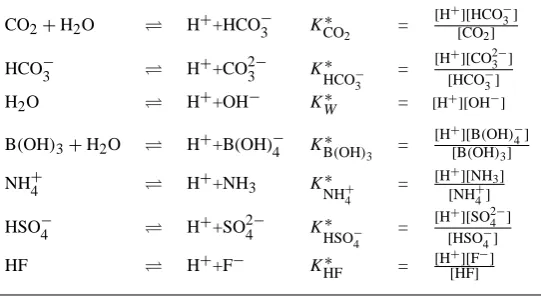
Table 3. Left: acid-base equilibria in the model. Right: definition of dissociation constants (stoichiometric equilibrium constants). Values

are calculated from temperature, salinity and pressure based on literature expressions (K∗

HSO−₄: Dickson (1990b);K

∗

HF: Dickson and Riley

(1979);K_CO∗ 2 andK

∗

HCO−₃: Roy et al. (1993), with extension for whole salinity range as given in Millero (1995);K

∗

W: Millero (1995);

K_B∗_(OH)

3: Dickson (1990a);K ∗

NH+₄: Millero (1995)). All stoichiometric equilibrium constants were converted to the free proton scale, and

pressure corrected according to Millero (1995) using the mean estuarine depth for each model box. Subsequently, they are converted to volumetric units using the temperature and salinity dependent formulation for seawater density according to Millero and Poisson (1981).

CO2+H2O H++HCO−3 K

∗

CO2 =

[H+][HCO−₃] [CO2]

HCO−₃ H++CO2₃− K∗

HCO−₃ =

[H+_][CO2− 3 ] [HCO−₃] H₂O H++OH− K_W∗ = [H+][OH−] B(OH)₃+H₂O H++B(OH)−₄ K_B∗_(OH)

3 =

[H+_][B

(OH)−₄] [B(OH)3]

NH+₄ H++NH₃ K∗

NH+₄ =

[H+][NH3] [NH+₄] HSO−₄ H++SO2₄− K∗

HSO−₄ =

A. F. Hofmann et al.: pH modelling with time variable acid-base constants 1543 available [TA] data, and subsequently, the [P_CO

2] values

were adjusted to provide the best fit. These [P_CO

2] values

calibrated for the year 2003 were subsequently used for all other years. To be consistent with pH boundary conditions available for all modelled years, [TA] boundary conditions were not directly calibrated from available 2003 [TA] mea-surements within the estuary, but calculated from calibrated [P

CO2] values and available pH boundary conditions

ac-cording to the total alkalinity definition used in our model (see below).

2.4 pH modelling approaches

In a recent review paper on pH modelling, we showed that there are two main approaches to calculate pH in a reactive transport model of an aquatic ecosystem (Hofmann et al., 2008a). These two methods can be referred to as implicit and explicit. The implicit method is the conventional pH modelling approach. This paper advances a new (extended) version of the explicit approach. To verify their consistency, we implemented both approaches side-by-side.

2.4.1 The implicit pH modelling approach

The implicit approach is the traditional method, which goes back to the work of Ben-Yaakov (1970) and Cul-berson (1980), and also forms the standard approach in-cluded in textbooks on aquatic geochemistry (Millero, 2006; Sarmiento and Gruber, 2006). The more recent treatments of the pH modelling problem by Luff et al. (2001) and Follows et al. (2006) are also based on this implicit method. Further-more, within the context of estuarine modelling, the implicit approach has been used by Regnier et al. (1997) and Vander-borght et al. (2002), and we also implemented it in our pre-vious paper on the biogeochemistry of the Scheldt estuary (Hofmann et al., 2008b). The implicit approach is termed ”implicit” because it essentially takes a detour via alkalin-ity to arrive at pH. In other words, one first expresses how biogeochemical processes affect the alkalinity mass balance (last equation in Table 2), and subsequently, at every time step, one calculates the pH from alkalinity and other total quantities (i.e. total carbonate, total borate, etc.). The lat-ter step comes down to the solution of a non-linear equation system governed by the mass action laws of the acid-base re-actions (as given in Table 3). Because of this two-step proce-dure, there is no direct link between biogeochemical process rates and the actual proton production or consumption these processes generate. As discussed extensively in Hofmann et al. (2008a), this is a clear drawback of the implicit ap-proach, since it does not allow the modeller to quantify how important an individual process really is in the total proton balance of the system.

2.4.2 The explicit pH modelling approach

Extending and improving the work of Jourabchi et al. (2005) and Soetaert et al. (2007), we recently presented a new ap-proach to pH calculations in reactive transport models (Hof-mann et al., 2008a). This method, called explicit here, al-lows us to describe the pH evolution over time (just like the implicit method), but in addition, it derives the contribution of separate biogeochemical processes to the overall rate of change of the proton concentration. First, we briefly review the main features of the explicit pH method as it was pre-sented in (Hofmann et al., 2008a), where it was assumed that dissociation constants remain constant in time. Subse-quently, we discuss how the method can be generalized to time-variable dissociation constants, which is the novel as-pect here.

The central idea of the explicit pH modelling method is that the total rate of change of the proton concentration can be written as

d[H+]

dt =

X

i

d[H+] dt i

(1)

where d[_dtH+]

i expresses the contribution of i-th process

(e.g. nitrification, CO2degassing, etc.). This partitioning of

the total rate of change of the proton concentration into sepa-rate contributions by different processes thus quantifies how important a given process is in the overall production and consumption of protons.

The definition of total alkalinity [TA] (Dickson, 1981) that is associated with the acid-base reaction set (Table 3) in our biogeochemical model is

[TA] =[HCO−₃]+2[CO2₃−]+[B(OH)−₄]+[OH−] + [NH3] −[H+]−[HSO−₄]−[HF]

(2) If one assumes that the acid-base reactions are in equilibrium, then each of the dissociated species on the right hand side can be expressed as a function of the proton concentration[H+], the concentrations of the total quantities[Xj]from

X=nXCO2,

X

NH+₄,XHSO−₄,XB(OH)3,

X

HFo (3) and some associated dissociation constantsK_i∗.

K∗=nK_CO2∗ , K∗

HCO−₃, K

∗

B(OH)3, K ∗

W, K

∗

NH+₄, K

∗

HSO−₄, K

∗

HF

o

(4) As a consequence, total alkalinity can be written as

1544 A. F. Hofmann et al.: pH modelling with time variable acid-base constants

Table 4. Process specific terms in Eqs. (8) and (14). Process rates: Tr = advective-dispersive transport, ECO2 = CO2degassing, ROx= oxic mineralisation, RNit= nitrification, RPP= primary production. Short notations:K∗(T )= changes in dissociation constants via changes

in temperature,K∗(S)= changes in dissociation constants via changes in salinity,K∗([P

HSO−₄])= changes in dissociation constants via changes in[P

HSO−₄],K∗([P

HF])= changes in dissociation constants via changes in[P HF].

d[H+_]

dt Tr =

TrTA −

P

j

TrXj ∂[TA]

∂[Xj]

.

∂[TA]

∂[H+_] (15)

d[H+_]

dt E_CO2 =

−ECO2

∂[TA]

∂[P CO2]

._∂[TA]

∂[H+_] (16)

d[H+_]

dt ROx

=ROx −

ROxCarb_∂[∂P[TA] CO2]

+ROx_∂[P∂[TA]

NH+₄]

._∂[TA]

∂[H+_] (17)

d[H+_]

dt RDen

=

0.8RDenCarb+RDen −

RDenCarb_∂[∂P[TA] CO2]

+RDen_∂[P∂[TA]

NH+₄]

.

∂[TA]

∂[H+_] (18)

d[H+_]

dt RNit

=

−2RNit −

−RNit_∂[P∂[TA]

NH+₄]

.

∂[TA]

∂[H+_] (19)

d[H+_]

dt RPP =

−

2pN−1

RPP −

−RPPCarb_∂[∂P[TA] CO2]

−pNRPP_∂[P∂[TA]

NH+₄] .

∂[TA]

∂[H+_] (20)

d[H+_]

dt K∗_{(T )} =

− dT dt P i _∂K∗ i ∂T

∂[TA]

∂K∗

i

.

∂[TA]

∂[H+_] (21)

d[H+_]

dt K∗_(S) =

−dS

dt P i _∂K∗ i ∂S

∂[TA]

∂K∗

i

._∂[TA]

∂[H+_] (22)

d[H+_]

dt K∗_([P

HSO−₄]) =

−

_d[P HSO−₄]

dt

P

i

∂K_i∗ ∂[P

HSO−₄]

∂[TA]

∂K∗

i

.

∂[TA]

∂[H+_] (23)

d[H+_]

dt K∗_([P

HF]) =

−d[

P HF] dt P i _∂K∗ i ∂[P

HF]

∂[TA]

∂K∗

i

._∂[TA]

∂[H+_] (24)

If one assumes that the dissociation constantsK_i∗do not depend on time, the time derivative of the total alkalinity can be specified as

d[TA]

dt =

∂[TA] ∂[H+_]

d[H+] dt +

X

j ∂[TA] ∂[Xj]

d[Xj]

dt (6)

This expression can be directly rearranged so that it provides an expression for the total rate of change of protons

d[H+]

dt =

d[TA] dt −

X

j ∂[TA] ∂[Xj]

d[Xj] dt

!

∂[TA]

∂[H+_] (7)

By plugging the expressions ford[_dtTA]and d[Xj]

dt given in

Ta-ble (2) into Eq. (7) and regrouping terms, we arrive at

d[H+] dt =

d[H+] dt Tr

+d[H

+_]

dt E_CO2

+d[H

+_]

dt ROx

+

d[H+] dt RDen

+d[H

+_]

dt RNit

+d[H

+_]

dt RPP

(8)

where the terms on the right hand side are given in Table 4 (Eqs. 15 to 20). This expression matches our sought-after expression Eq. (1). If the acid-base dissociation constants can be assumed constant over time, this expression allows us to individually quantify the contributions of oxic minerali-sation, denitrification, nitrification, primary production, air-water exchange and advective-dispersive transport to the rate of change of the proton concentration. Note that the acid-base dissociation constants should only be independent of

time (accordingly, a stationary spatial gradient in these con-stants does not pose a problem). In the following section, we introduce the novel aspect of this publication: we describe how to apply the explicit pH modelling approach to a system with time variable acid-base dissociation constants.

2.4.3 The explicit pH modelling approach with time variable dissociation constants

For a number of problems in aquatic biogeochemistry, the assumption of time-invariant acid-base dissociation con-stants is not tenable. Estuaries form a prime example of this. Because salinity and temperature show a marked sea-sonal dependence, the acid-base dissociation constants will also change over time. When accounting for this time-dependency, one should account for the direct effect of tem-peratureT, salinitySand pressureP on the dissociation con-stants

K_i∗=fi(T , S, P ) (9)

A. F. Hofmann et al.: pH modelling with time variable acid-base constants 1545 1984; Zeebe and Wolf-Gladrow, 2001)

K_i∗,free=K_i∗,SWS



1+ [P

HSO−₄] K∗,free

HSO−₄ +[

P_HF] K_HF∗,free



 (10)

This implies that, in general, the dissociation constants are also functions of[P

HSO−₄]and[P

HF] K_i∗=fi(T , S,[

X

HSO−₄],[XHF]) (11) Note that if one assumes that[P

HSO−₄] and[P

HF] are simply proportional to S,[P_HSO−

4]and[

P_{HF]need not}

to be treated as independent variables. However, to pre-serve the generic nature of the presented method, we treat S,[P

HSO−₄], and[P

HF]as independent variables in the derivations below. Accordingly, if one assumes thatT, S,

[P

HSO−₄], and[P

HF]are dependent on time, and so the dissociation constants K_i∗ become dependent on time, the time derivative of total alkalinity (Eq. 5) now provides the more elaborate expression

d[TA] dt =

∂[TA] ∂[H+_]

d[H+] dt +

X

j

_∂[TA] ∂[Xj]

d[Xj] dt + X i

∂[TA] ∂K_i∗

∂K_i∗ ∂T dT dt+ X i

∂[TA] ∂K_i∗

∂K_i∗ ∂S dS dt+ X i

[TA] ∂K_i∗

∂K_i∗

∂[P

HSO−₄] !

d[P

HSO−₄]

dt +

X

i

_[TA] ∂K_i∗

∂K_i∗ ∂[P_HF]

_d[P

HF] dt

(12)

Appendix A details how the partial derivatives in this expres-sion can be explicitly calculated as a function of the proton concentration, the total quantities Xj and the dissociation

constantsK_i∗. Again, Eq. (12) can be directly transformed into following expression for the total rate of change of pro-tons

d[H+_]

dt =

d[TA]

dt −

P j

∂[TA]

∂[Xj]

d[Xj]

dt + P i _∂ [TA] ∂K∗ i ∂K∗ i ∂T dT dt+ P i ∂[TA]

∂K_i∗ ∂K∗_i

∂S dS dt+ P i ∂[TA]

∂K∗

i

∂K_i∗ ∂[P

HSO−₄]

d[P HSO−₄]

dt +

P i

∂[TA]

∂K_i∗ ∂K∗

i

∂[P HF]

_d[P HF]

dt

∂[TA]

∂[H+_] (13)

In a similar way as above, one can plug the expressions for

d[TA]

dt , and d[Xj]

dt as given in Table 2 into Eq. (13) and

rear-range the terms so that terms associated with a given process are grouped together. This leads to

d[H+]

dt = d[H+]

dt Tr+ d[H+]

dt E_CO2+ d[H+]

dt ROx+

d[H+]

dt RDen+

d[H+_]

dt RNit

+d[H+] dt RPP

+d[H+] dt K∗_{(T )}+

d[H+_]

dt K∗_(S)+

d[H+_]

dt K∗₍[P

HSO−₄])+ d[H+_]

dt K∗₍[P HF])

(14)

with process specific terms as given in Table 4. In addition to the processes already featuring in Eq. (8), there are now ad-ditional contributions related to the effect of changing tem-perature and salinity (Eqs. 21 and 22), as well as two terms linked to pH scale conversion (Eqs. 23 and 24).

2.5 Model implementation

The biogeochemical reactive transport model and the pH cal-culation procedures were implemented in FORTRAN within the ecological modelling framework FEMME (Soetaert et al., 2002). The model code is an extension of the code discussed in (Hofmann et al., 2008b). As noted above, the implicit pH calculation routine was already present in this code and has been retained. Here, the code was extended with the explicit pH modelling method as described in Sect. 2.4.3. Accord-ingly, the model code implements two different pH calcula-tion procedures, which independently predict the pH evolu-tion of the estuary, thus allowing for a consistency check be-tween these two methods. The model code can be obtained from the corresponding author or from the FEMME website: http://www.nioo.knaw.nl/projects/femme/. Post processing of the model results and visualization of the model output was done using the programming languageR (R Develop-ment Core Team, 2005).

2.6 Model simulations

2.6.1 Baseline simulation, calibration, generation of output

The baseline simulation is the model solution that best fits the data. It is used as the starting point for the subsequent sen-sitivity analysis. To arrive at the baseline simulation, a time dependent simulation over a four year period was performed spanning the years from 2001 to 2004. Boundary condi-tions (values for [TA], S, [P

NH+₄], [OM], [O2], [NO−₃], [P

HSO−₄],[P

B(OH)3], and[PHF], temperature, and the

freshwater flow) were imposed onto the model with monthly resolution, using the data as described in Sect. 2.2. The initial conditions for this time dependent simulation were obtained by a steady state model run, where all boundary conditions were fixed at January 2001 values. The state variable[H+_] (for the explicit pH modelling approach) has been initialized with an implicitly calculated initial pH. The model was nu-merically integrated over time with an Euler scheme using a time-step of 0.00781 days. To be comparable to NIOO mon-itoring pH data (measured on the NBS pH scale), the simu-lated pH values (calcusimu-lated on the free pH scale) were con-verted to the NBS scale using the Davies equation (cf. dis-cussion of the use of the Davies equation in Hofmann et al., 2008b).

1546 A. F. Hofmann et al.: pH modelling with time variable acid-base constants

0 20 40 60 80 100

7.5

7.6

7.7

7.8

7.9

8.0

8.1

0 20 40 60 80 100 0 20 40 60 80 100 0 20 40 60 80 100

PSfrag

replacemen

ts

river km

pH

(NBS

scale)

2001 2002 2003 2004

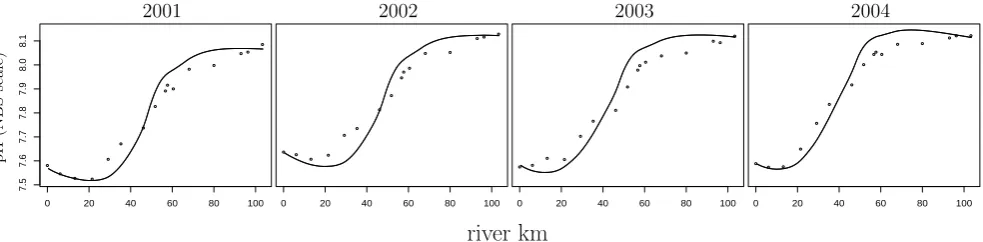
Fig. 2. The model fit for pH for the modelled years 2001 through 2004. The dots represent NIOO monitoring data on the NBS scale (see

Hofmann et al., 2008b), the lines represent modelled pH (modelled free scale pH values have been converted to the NBS scale using the Davies equation – cf. discussion of the use of the Davies equation in Hofmann et al., 2008b).

nitrification rates. First, the data for the year 2003 were used to calibrate the process rate parameters of the model in a run that covered the year 2003 only. Subsequently, data for the remaining years (2001, 2002, and 2004) were used to inde-pendently validate the model in the above mentioned four-year run (keeping rate parameters at values calibrated for 2003, but changing boundary conditions and physical forc-ings to values of the respective years). In addition, nitrifica-tion rates for the year 2003 were taken from Andersson et al. (2006) and were used to independently validate the model. Additional details on data sources, analytical methods and model calibration, as well as fits of model output to data other than pH can be found in Hofmann et al. (2008b).

To arrive at yearly-averaged, longitudinal profiles, the model output (concentrations, process rates, pH) of the time-dependent simulation for every model box was suitably av-eraged over the desired period. A similar procedure was ap-plied to the monthly monitoring data. We also created vol-ume integrated, “per model box” longitudinal profiles. To this end, the volumetric rates as calculated with Eqs. (13) to (22) were multiplied with the volume of the respective model box along the river. Subsequently, we then integrated longitudinally to arrive at ”whole estuarine” process rates, i.e. we multiplied the rates for each model box with the vol-ume of the respective box and summed up. We also averaged longitudinally to arrive at “mean eastuarine” values of con-centrations, pH, and process rates. To this end, the value in each model box was weighted with the volume of that box, summed up and divided by the total estuarine volume. Ad-ditionally, all obtained profiles, mean and total values have been averaged over the four modelled years.

Figure 2 shows the resulting yearly-averaged pH profiles of the baseline simulation. The final pH fit shows a slight underestimation of pH in the upstream region and a slight overestimation in the downstream region. This could most probably be remedied with a more elaborate model includ-ing additional biogeochemical processes and a more elabo-rate hydrology (migrating from a one-dimensional model to

two or even three dimensions). However, to get an idea about the dynamic equilibrium that maintains the pH along the es-tuary, we consider the present model elaborate enough and the resulting fit good enough.

2.6.2 pH modelling verification runs

The implicit and explicit pH modelling approaches are two different methods for calculating the same quantity. This means that if these two methods are implemented correctly, they must produce exactly the same pH response (provided the underlying biogeochemical model is exactly the same, as is the case here). This was verified by executing the base-line simulation with both the implicit method and the ex-plicit pH modelling method with time-variable dissociation constants as in Sect. 2.4.3. These two methods provide in-deed the same response within the numerical precision of the code, as shown in Fig. 3c for the year 2003 (the other 3 years show a similar response).

Some details warant further discussion. The extended explicit pH modelling method presented here explicitly ac-counts for time-variable acid-base dissociation constants. This adds a number of d[_dtH+]

i terms to the proton balance

equation (compare Eq. (8) to Eq. (14)). It is useful to rewrite Eq. (14) in following form

d[H+]

dt =

X

i

_d[H+_]

dt prodi

−X

i

_d[H+_]

dt consi

+1

=P P −P C+1

(25)

TheP P andP Cterms gather all proton producing and con-suming processes given in Eq. (8). The 1 stands for all terms that are present in Eq. (14) but not in Eq. (8). The

1 term includes terms that account for two effects: time-dependent changes in salinity and temperature, which influ-ence the dissociation constants directly, and time-dependent changes in[P

HSO−₄]and[P

A. F. Hofmann et al.: pH modelling with time variable acid-base constants 1547

0 20 40 60 80 100

7.6

7.8

8.0

8.2

8.4

0 20 40 60 80 100 0 20 40 60 80 100

PSfrag

replacemen

ts

river km

pH

(NBS

scale)

A B C

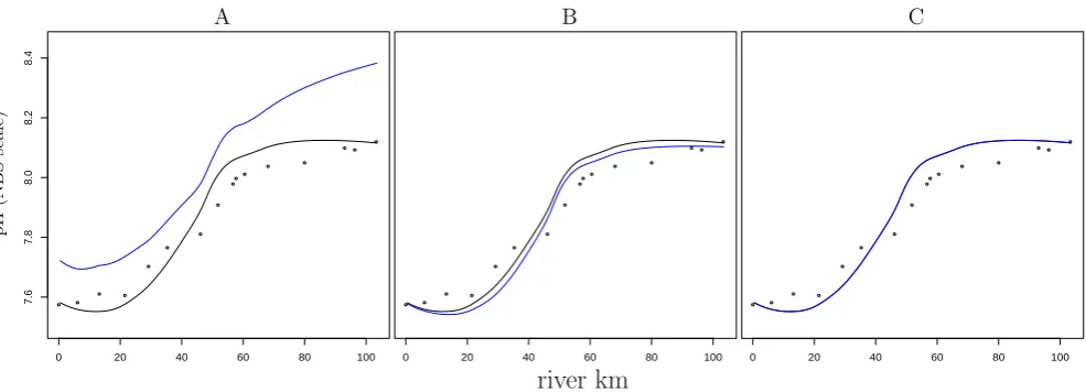
Fig. 3. Verification of the explicit pH modelling method using model runs for the year 2003. The black dots represent NIOO monitoring

data (see Hofmann et al., 2008b), the black lines represent modelled pH calculated with the implicit approach and the blue lines represent modelled pH calculated with the explicit approach (modelled free scale pH values have been converted to the NBS scale using the Davies equation (cf. discussion of the use of the Davies equation in Hofmann et al., 2008b)). (a): omitting allK∗related terms from Eq. (14); (b): considering the terms describing the variations in the dissociation constants due to changes inSandT but without the pH scale conversion related terms; (c): considering all terms as described in Sect. (2.4.3).

As shown below, the proton productionP Pand the proton consumptionP C are very large compared to the net rate of change of protonsd[_dtH+], and as a result,P P andP Calmost balance each other. Additionally, the1term is also small compared toP P andP C. Accordingly, one is tempted to omit 1 from Eq. (14). Yet, we found that such an omis-sion introduces substantial deviations as shown in Figs. 3a, b. Omitting all terms in1from Eq. (14), yields pH profiles that are substantially different from the correctly calculated ones (Fig. 3a). Including the terms that account for the di-rect effect of temperature and salinity (but not including the pH scale effect) yields a better result (Fig. 3b). However, a small deviation is still present. Additionally including the pH scale conversion related terms makes the response of the explicit method identical to the the implicit one, as required (Fig. 3c).

To explain why the neglect of very small terms in1(so small that they irrelevant when comparingP P andP C and the contributions of individual processes therein) can have relatively large consequences, one must realize thatP P and

P C are very large compared to the net rate of change of protons d[_dtH+]. Accordingly, a small disturbance of this bal-ance (like ignoring1) can have a huge impact ond[_dtH+], and hence, on the model predicted pH value. This explains the deviations in Fig. 3. In conclusion, the explicit pH modelling method is powerful, but one needs to ensure that it is consis-tently implemented and no terms are omitted.

0 5 10 15 20 25

3000

3500

4000

4500

3000

3500

4000

4500

7.6

7.8

8.0

8.2

PSfrag

replacemen

ts

pH

(NBS)

[ _P

CO

2]

[T

A]

S

µ

mol/kg-soln

Fig. 4. Basic model simulation with no salinity dependence of the

acid-base constants (values were calculated atT=15◦C andS=15), no gas exchange, and no biogeochemistry. [P

CO2], [TA] and pH

(NBS) are plotted along the estuary as a function of salinity. The pH from upstream to downstream increases as a result of a de-crease in the ratio between[P

CO2]and [TA]. End-members for

[P

CO₂], [TA], andSare the upstream and downstream values for 2001 in the baseline model run. Due to the simplicity of the re-maining model formulation the calculations are performed using an

Rscript (R Development Core Team, 2005) and the acid-base mod-elling packageAquaEnv(Hofmann et al., submitted) instead of the full FORTRAN implementation of the model.

2.6.3 Sensitivity analysis

1548 A. F. Hofmann et al.: pH modelling with time variable acid-base constants

0 5 10 15 20 25

7.4

7.6

7.8

8.0

8.2

0 5 10 15 20 25

7.4

7.6

7.8

8.0

8.2

0 5 10 15 20 25

7.4

7.6

7.8

8.0

8.2

0 5 10 15 20 25

7.4

7.6

7.8

8.0

8.2

0 5 10 15 20 25

7.4

7.6

7.8

8.0

8.2

PSfrag

replacemen

ts

pH

(NBS)

pH

(NBS)

pH

(NBS)

pH

(NBS)

pH

(NBS)

S S S S S

closed system, no biology open system, no biology closed system, biology full biogeochemical model

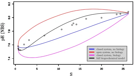
Fig. 5. pH profiles along the Scheldt estuary salinity gradient. The

blue line represents the pH calculated with a closed system model without biology (comparable to Mook and Koene, 1975); the red line represents the pH calculated with an open system model with-out biology (comparable to Whitfield and Turner (1986) but with realistic kinetic CO2air-water exchange instead of a fully

equili-brated system); the magenta line represents a closed system model with biology; the black line represents the pH calculated with the full biogeochemical model as presented in Hofmann et al. (2008b). All models are based on 2001 parameter values. The black circles are the observed pH data for 2001.

sequentially activated to arrive at more biogeochemically complex scenarios. The basic scenario simply served to in-vestigate the effect of estuarine mixing on the pH profile. To this end, we purposely neglected gas exchange (CO2and O2)

and biological processes, and assumed no dependence of the stoichiometric constants on salinity (values were calculated atT=15◦_{C andS=15). Accordingly, in this basic scenario,} the pH profile along the estuary is solely determined by con-servative mixing of [TA] and[P_CO

2], driven by the

differ-ence in upstream and downstream boundary values (Fig. 4). Starting from this basic scenario, we conducted four addi-tional simulations where groups of processes where sequen-tially activated. In a first scenario, gas exchange and biologi-cal processes where still neglected (“closed system, no biol-ogy”), but the salinity dependence of the stoichiometric con-stants was now explicitly accounted for. In two subsequent simulations, either gas exchange was additionally activated (“open system, no biology”) or biological processes were included (“closed system, biology”). In a fourth and final simulation, all processes were activated thus leading to the baseline simulation as discussed above (“full biogeochemi-cal model”). To be comparable to the work of Mook and Koene (1975), the resulting pH profiles are plotted against the salinity gradient in the estuary (Fig. 5).

2.6.4 Factors governing changes in the mean estuarine pH from 2001 to 2004

Hofmann et al. (2008b) reported an upward trend in the mean estuarine pH over the years 2001 to 2004, but did not investi-gate the underlying causes of this trend. Potential factors are

a different temperature forcing, changes in freshwater input (modifying the salinity gradient and the concentrations of all chemical species in the estuary), or temporal variations in the chemical composition of the water at the boundaries. Table 5 shows the inter-annual variations of these factors as well as variations in values of important state variables volume av-eraged over the whole estuary. We carried out a sensitivity analysis to find out which particular factors could explain the observed four-year pH trend.

Because the temperature follows a predictable seasonal cy-cle, inter-annual changes in the temperature forcing are neg-ligible. Model runs with all parameters fixed at the 2001 values, but with the actual time-variable temperature forcing from 2001 to 2004, show no discernably different pH profile. This leaves to investigate the effect of changing freshwater input and changing boundary concentrations. We suspected that the biogeochemistry of a particular compound was pre-dominantly influenced by changes in its total “load”, i.e., the total input at the upstream boundary. For example, the am-monia load is simply defined as the freshwater dischargeQ

times the upper boundary concentration[P

NH+₄]_up. In our sensitivity analysis, we were particularly interested which loading changes (i.e. of which chemical variable) were re-sponsible for the observed inter-annual pH changes.

In the baseline simulation described above, boundary con-ditions and freshwater discharge vary simultaneously over time, forced by the monthly monitoring data. To disentangle the effects of freshwater discharge and boundary changes on the total loading, we executed 14 simulations in which the freshwater discharge or the boundary concentration values (upstream and downstream) were independently varied. In these simulations, all other state variables remained at 2001 values. Table 6 lists the groups of state variables for which the loading has changed, either by changing the freshwater flow (left column) or the boundary conditions (right column). Each time the resulting pH change of the four year period was expressed as a fraction of the pH change arrived at in the baseline scenario to quantify the importance of the given parameter change in explaining the four-year pH trend.

3 Results

3.1 Factors controlling the pH profile along the estuary We performed a number of exploratory simulations to inves-tigate the major controls on the longitudinal pH profile in the Scheldt estuary, which is also characteristic for other estu-aries. A first striking aspect is that the pH increases from the upstream freshwater boundary to the downstream marine boundary. A “skeleton” simulation (with no gas exchange, no biogeochemistry and no dependence of acid-base con-stants on salinity) shows that this pH increase is simply the result of conservative mixing of [TA] and[P

CO2], as the

ratio[P

A. F. Hofmann et al.: pH modelling with time variable acid-base constants 1549

Table 5. Model forcings (upper part of the table) and a selection of mean estuarine model values resulting from the baseline simulation

(lower part of the table). The subscript “up” denotes upstream boundary condition , the subscript “down” denotes downstream boundary condition. The boundary conditions for[TA]are calculated from boundary values for [P

CO2] in combination with pHup and pHdown

(which are otherwise not used as boundary conditions). Concentrations are given in mmol m−3, the flow at the upstream boundaryQis given in m3s−1. The pH output from the model simulations is converted to the NBS scale to be comparable with the data.

2001 2002 2003 2004 freshwater flow (Q) 190 184 112 95

pHup(NBS) 7.574 7.638 7.586 7.591

pHdown(NBS) 8.069 8.124 8.117 8.114

[P

CO2]up 4700 4700 4700 4700

[P

CO2]down 2600 2600 2600 2600

[TA]_up 4441 4493 4470 4473

[TA]_down 2702 2728 2726 2733

Sup 0.6 0.6 0.9 1.0

Sdown 26.5 27.7 28.3 30.2

[P

NH+₄]_up 110 105 118 72

[P

NH+₄]_down 8 4 6 4

[FastOM])up+ [SlowOM])up 41 49 54 55

[FastOM])down+ [SlowOM])down 10 10 7 9

[O2]up 94 76 71 65

[O2]down 293 272 280 268

pH (NBS) 8.010 8.053 8.069 8.095

[P

CO2] 2872 2881 2818 2795

[TA] 2918 2951 2902 2898

[P

NH+₄] 10.4 9.1 9.5 6.8

Table 6. Model scenarios to investigate the trend in the mean estuarine pH over the years 2001 to 2004. Changes in the total “loading” for

particular chemicals either due to changes in the freshwater discharge (left column) or due to changes in the boundary concentrations (right column). The entries indicate the variables for which the loading has changed, while all other loadings have been fixed at 2001 values. Note that in all these scenarios, [TA] boundary conditions are calculated consistently from pH boundary forcing values.

loading change via discharge loading change via boundary concentrations a) all state variables h) all state variables

b) [P

CO2],[TA] i) [TA](pH)

c) S j) S

d) [P

NH+₄] k) [P

NH+₄]

e) [FastOM],[SlowOM] l) [FastOM],[SlowOM]

f) [O2] m) [O2]

g) [NO−₃],[P

HSO−₄],[P

B(OH)3],[PHF] n) [NO−3],[

P

HSO−₄],[P

B(OH)3],[PHF]

On top of the overall increase in pH, the observed pH pro-file shows a changing curvature with a distinct pH minimum at low salinities. Via a sensitivity analysis, we examined how strongly different groups of processes (salinity dependence of acid-base constants, gas exchange, biology) influence the shape of the longitudinal pH profile. Figure 5 shows that the simulation, which considers a closed system (no CO2

and O2 exchange with the atmosphere) and no biological

processes, exhibits a distinct pH minimum at low salinities (blue line). However this simulated pH minimum is located at higher salinities (more downstream) than the observed pH

1550 A. F. Hofmann et al.: pH modelling with time variable acid-base constants at low salinities, the data pH profile shows less curvature at

high salinities).

3.2 Proton production and consumption along the estuary

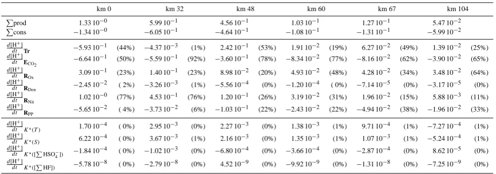
The prime advantage of the explicit pH modelling method is that it calculates the proton production/consumption rates as-sociated with each individual reactive transport process. Fig-ure 6a shows the contributions of individual processes to the net rate of change of protons as calculated with Eqs. (13) to (22). Longitudinal profiles of proton production or consump-tion rates (per unit of soluconsump-tion volume) were extracted from the baseline simulation, averaged over the four year period (for every model box), and plotted cumulatively. Table 7 lists resulting values at selected positions (model boxes) in the river where the pH profiles in Fig. 6 show interesting fea-tures (these locations are also indicated in Fig. 1).

In a first step, we can look at the overall proton cycling, i.e., the total proton production (P P) and total proton con-sumption (P C) along the estuary. A first observation is that theP P andP Cterms are always four to five orders of mag-nitude larger than the actual rate of change of protons (which is in the 10−5 _{mmol m}−3 _{range). This implies that proton}

production and consumption are nearly balanced, and that the internal cycling of protons far outweighs the net proton change over time. A second aspect is that the proton pro-duction rates, which are linked to changes in the dissociation constants, are about three orders of magnitude smaller than those of other processes. Therefore, they are not presented in Figs. 6 and 7. Yet, as noted above, incorporation of these in-fluences is necessary for a consistent implementation of the explicit pH approach (i.e. to model absolute pH values cor-rectly).

As shown in Fig. 6a, the proton production and consump-tion per unit volume shows a marked decrease in the upper half of the estuary (between river km 0 and 60), after which the decrease proceeds more gradually. Over the whole es-tuary,P P andP C decrease by a factor of 20, from around 1.3 mmol m−3yr−1to 0.06 mmol m−3yr−1. This decrease in proton turn-over generates the trumpet-like shape in Fig. 6a, and can be attributed to a similar decreasing trend in the bio-geochemical activity per volume of solution (as discussed be-low).

Along the estuary, the magnitude of the individual con-tributions d[_dtH+]

i generally follows the decreasing trend in

the total proton production/consumption. The exceptions are primary production, whose proton consumption remains rel-atively constant, and advective-dispersive transport, which shows a noticeable profile (further discussed below). How-ever, there are some marked changes in the relative impor-tance of processes in the overall proton cycling. Nitrifica-ton and oxic mineralisation produce proNitrifica-tons; CO2degassing,

primary production, and denitrification consume protons. The dominant proton producer at the upstream boundary is

nitrification (77%), yet its relative importance drops to 11% downstream. In parallel, the relative importance of oxic mineralisation as a proton producer increases from 23% up-stream to 64% at the downup-stream boundary. In terms of proton consumption, the most important process is CO2

de-gassing. Its relative importance increases from 50% at the upstream boundary to 92% at km 32 and then decreases again to 65% at the downstream boundary. Compared to CO2

de-gassing, the proton consumption by primary production is small. The relative importance of primary production as a proton consumer increases from 4% at the upstream bound-ary to 38% at km 67 and decreases again to 33% at the down-stream boundary. The proton consumption due to denitrifica-tion is not important in the Scheldt estuary (around 1% along the estuary).

The role of advective-dispersive transport in proton trans-port is markedly different from that of the biogeochemical re-actions. Advective-dispersive transport counteracts the dom-inant proton consuming or producing processes. As a result of that, it switches sign. Around river km 32, it switches from proton consumption (importing protons into a model box) to proton production (exporting protons from a model box). Moreover, its rate does not change monotonically. Pro-ton production due to advective-dispersive transport shows a maximum around river km 48 and a secondary maximum around river km 67. At the upstream boundary advective-dispersive transport accounts for 44% of the proton con-sumption, while downstream it accounts for about 25% of the proton production.

Figure 6b shows the longitudinal profile of the volume-integrated proton production and consumption rates (ex-pressed “per model-box”). Table 8 lists selected values along the estuary. The cross section area increases from around 4000 m2 upstream to around 76 000 m2 downstream, while the mean estuarine depth remains approximately constant around 10 m. As a result, there is a much larger estuar-ine volume in the downstream model boxes than in the up-stream model boxes. This volume increase per box com-pensates for the decrease in the rates per unit volume. As a consequence, the volume-integrated proton production or consumption rates in Fig. 6b remain similar along the estu-ary. The mid-region of the estuary (between kms 30 and 60) emerges as the most important region for volume integrated proton cycling. In this area the proton budget is dominated by the physical transport processes: CO2air-water exchange

and advective-dispersive transport. The volume-integrated proton production/consumption of oxic mineralisation, pri-mary production and CO2degassing is clearly larger

A. F. Hofmann et al.: pH modelling with time variable acid-base constants 1551

Table 7. Contributions of various biogeochemical processes to the proton cycling per unit of solution volume; values in mmol H+m−3y−1; percentages are of total production (positive quantities) or consumption (negative quantities), respectively.

km 0 km 32 km 48 km 60 km 67 km 104

P

prod 1.33 10−0 5.99 10−1 4.56 10−1 1.03 10−1 1.27 10−1 5.47 10−2

P_{cons −1.34 10}−0 _{−6.05 10}−1 _{−4.64 10}−1 _{−1.08 10}−1 _{−1.31 10}−1 _{−5.99 10}−2

d[H+_]

dt Tr −5.93 10−1 (44%) −4.37 10−3 (1%) 2.42 10−1 (53%) 1.91 10−2 (19%) 6.27 10−2 (49%) 1.39 10−2 (25%)

d[H+_]

dt ECO2 −6.64 10

−1 _{(50%) −5.59 10}−1 _{(92%) −3.60 10}−1 _{(78%) −8.34 10}−2 _{(77%) −8.16 10}−2 _{(62%) −3.90 10}−2 _(65%)

d[H+_]

dt ROx 3.09 10

−1 _{(23%) 1.40 10}−1 _{(23%) 8.98 10}−2 _{(20%) 4.93 10}−2 _{(48%) 4.28 10}−2 _{(34%) 3.48 10}−2 _(64%)

d[H+_]

dt RDen −2.45 10

−2 _{( 2%) −3.26 10}−3 _{(1%) −5.56 10}−4 _{(0%) −1.20 10}−4 _{( 0%) −7.14 10}−5 _{(0%) −3.17 10}−5 _(0%)

d[H+_]

dt RNit 1.02 10

−0 _{(77%) 4.53 10}−1 _{(76%) 1.20 10}−1 _{(26%) 3.19 10}−2 _{(31%) 1.96 10}−2 _{(15%) 5.88 10}−3 _(11%)

d[H+_]

dt RPP −5.65 10

−2 _{( 4%) −3.73 10}−2 _{(6%) −1.03 10}−1 _{(22%) −2.43 10}−2 _{(22%) −4.94 10}−2 _{(38%) −1.96 10}−2 _(33%)

d[H+_]

dt K∗

(T ) 1.70 10

−4 _{( 0%) 2.95 10}−3 _{(0%) 2.27 10}−3 _{(0%) 1.38 10}−3 _{(1%) 9.71 10}−4 _{(1%) −7.27 10}−4 _(1%)

d[H+_]

dt K∗_(S) 6.22 10−4 ( 0%) 3.67 10−3 (1%) 2.16 10−3 (0%) 1.35 10−3 (1%) 1.07 10−3 (1%) −5.24 10−4 (1%)

d[H+_]

dt K∗_([P

HSO−4])

−1.84 10−4 _{( 0%) −1.02 10}−3 _{(0%) −6.80 10}−4 _{(0%) −3.66 10}−4 _{(0%) −2.87 10}−4 _{(0%) 8.62 10}−5 _(0%)

d[H+_]

dt K∗_([P

HF]) −5.78 10

−8 _{( 0%) −2.79 10}−8 _{(0%) 4.52 10}−9 _{(0%) −9.92 10}−9 _{(0%) −1.31 10}−8 _{(0%) −7.25 10}−9 _(0%)

Table 8. Volume integrated proton budget; proton production/consumption rates in kmol H+y−1per model box.

km 0 km 32 km 48 km 60 km 67 km 104

P

prod 5.54 10−0 4.08 10−0 10.70 10−0 4.52 10−0 7.08 10−0 4.34 10−0 P

cons −5.57 10−0 −4.12 10−0 −10.90 10−0 −4.74 10−0 −7.32 10−0 −4.74 10−0

d[H+]

dt Tr −2.47 10

−0 _{−2.97 10}−2 _{5.70 10}−0 _{8.36 10}−1 _{3.50 10}−0 _{1.10 10}−0

d[H+_]

dt E_CO2 −2.76 10

−0 _{−3.81 10}−0 _{−8.48 10}−0 _{−3.66 10}−0 _{−4.55 10}−0 _{−3.09 10}−0

d[H+_]

dt ROx 1.29 10

−0 _{9.51 10}−1 _{2.11 10}−0 _{2.16 10}−0 _{2.39 10}−0 _{2.76 10}−0

d[H+]

dt RDen

−1.02 10−1 −2.22 10−2 −1.31 10−2 −5.24 10−3 −3.98 10−3 −2.51 10−3

d[H+]

dt RNit 4.25 10

−0 _{3.08 10}−0 _{2.81 10}−0 _{1.40 10}−0 _{1.09 10}−0 _{4.66 10}−1

d[H+_]

dt RPP

−2.35 10−1 −2.54 10−1 −2.42 10−0 −1.07 10−0 −2.75 10−0 −1.55 10−0

d[H+_]

dt K∗_{(T )} 7.09 10−4 2.01 10−2 5.34 10−2 6.03 10−2 5.41 10−2 −5.76 10−2

d[H+]

dt K∗_(S) 2.59 10−3 2.50 10−2 5.09 10−2 5.93 10−2 5.97 10−2 −4.15 10−2

d[H+_]

dt K∗_([P

HSO−₄]) −7.65 10

−4 _{−6.94 10}−3 _{−1.60 10}−2 _{−1.61 10}−2 _{−1.60 10}−2 _{6.83 10}−3

d[H+_]

dt K∗_([P

HF]) −2.41 10

−7 _{−1.90 10}−7 _{1.06 10}−7 _{−4.35 10}−7 _{−7.30 10}−7 _{−5.75 10}−7

3.3 Whole estuarine proton budget

Figure 7 shows a proton budget integrated over the whole model area and averaged over the four modelled years. It can be seen that CO2degassing and primary production are the

processes that net consume protons in the estuary (disregard-ing the minor contribution of denitrification). Nitrification is the main proton producer, followed by oxic mineralisa-tion and advective-dispersive transport. Note that the proton budget does not add up to zero, but a small negative value remains (−20 kmol[H+]estuary−1y−1). This indicates that the estuary as a whole, averaged over a year, is not

com-pletely in steady state. This is consistent with the upwards trend in the mean estuarine pH, which is observed in the data and in the model simulations.

1552 A. F. Hofmann et al.: pH modelling with time variable acid-base constants

0 20 40 60 80 100

−1.5

−1.0

−0.5

0.0

0.5

1.0

1.5

PSfrag

replacemen

ts

river km

mmol

H

+

m

−

3y

−

1

Tr ECO2

ROx

RDen

RNit

RPP

a)

0 20 40 60 80 100

−15

−10

−5

0

5

10

PSfrag

replacemen

ts

river km

kmol

H

+

mo

del-b

ox

−

1y

−

1

Tr

ECO2

ROx

RDen

RNit

RPP

b)

Fig. 6. The influences of kinetically modelled processes on the

pH – volumetrically a) and volume integrated b), averaged over the four modelled years. Note that the process abbreviations given in the legend represent the contribution of the respective process to d[_dtH+], e.g., Tr signifies d[H_dt+]_Tr. Process abbrevi-ations: Tr=advective-dispersive transport, ECO2=CO2 degassing, R_Ox=oxic mineralisation, R_Nit=nitrification, R_PP=primary produc-tion,K∗(T )=changes in dissociation constants via changes in tem-perature, K∗(S)=changes in dissociation constants via changes in salinity,K∗([P

HSO−₄])=changes in dissociation constants via changes in[P

HSO−₄],K∗([P

HF])=changes in dissociation con-stants via changes in[P

HF].

for each zone (Fig. 8). Because the decrease in the process rates from upstream to downstream is compensated by an in-crease in estuarine volume, the total proton production is of the same order of magnitude in the three zones. However, there are marked changes in the relative importance of pro-cesses.

Upstream, the proton production due to nitrification, and to a lesser extent oxic mineralisation, are counteracted by CO2 degassing and advective-dispersive transport. In the

midstream section, the contribution of aerobic respiration and advective-dispersive transport (which has now become a proton producer) are of similar magnitude as that of nitri-fication. In this midstream part, CO2 degassing is also the

major proton consuming process. In the downstream part of the estuary, nitrification is even less important, and the net proton production by oxic mineralisation as well as the

−600

−400

−200

0

200

123

−394

178

−2.13

202

−127

PSfrag

replacemen

ts

kmol

H

+

estuary

−

1y

−

1

Tr E_CO

2 ROx RDen RNit RPP

Fig. 7. Whole estuarine proton budget, averaged over the four

mod-elled years. The error bars represent the standard deviations result-ing from averagresult-ing over the four years. The process abbreviations in the legend denote the contribution of the respective biogeochemical process e.g., Tr refers tod[_dtH+]_Tr.

net consumption of protons by primary production gain more importance.

3.4 Factors responsible for the trend in the mean estuarine pH from 2001 to 2004

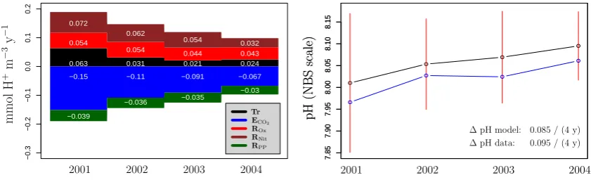
Figure 9 shows the trend in the mean estuarine pH over the four year period. Both the trend as derived from the data as well as the trend simulated by the model are shown. The pH changed by about 0.085 from 8.010 to 8.095 in the model, which is backed by a similar pH increase of 0.095 in the data. There is a small offset between model and data. This is because the model slightly underestimates the pH in the up-stream region with low estuarine volume and overestimates the pH in the downstream region with high estuarine volume. Because of volume averaging, the latter dominates the mean estuarine pH.

As a first step to investigate the underlying causes of this trend, we have plotted the volume integrated proton pro-duction/consumption for the individual years 2001 to 2004 alongside each other (the values displayed in Figs. 4, 5 and 6 were time averages over the whole four-year period). This shows that the overall proton turn-over decreased over the four-year period. The contributions of CO2 degassing and

nitrification steadily declined from 2001 to 2004 (with the decline being more pronounced for CO2 degassing). The

contribution from oxic mineralisation showed no clear trend, while the contribution of transport declined from 2001 to 2003 and then slightly increased again from 2003 to 2004.

A. F. Hofmann et al.: pH modelling with time variable acid-base constants 1553

−100

−50

0

50

100

−28 −85

26 −2

92 −4

−250

−200

−150

−100

−50

0

50

100

70 −163

47 0

77 −37

−200

−100

0

100

81 −146

104 0

33 −86

PSfrag

replacemen

ts

kmol

H

+

estuary

−

1y

−

1

kmol

H

+

estuary

−

1y

−

1

kmol

H

+

estuary

−

1y

−

1

Tr

E_CO

2

ROx

R_Den

R_Nit

R_PP

a) b) c)

Fig. 8. Proton budget for three different zones in the estuary: (a) upstream region between river km 0 and 30, (b) midstream region

between km 30 and 60, and (c) the downstream region, averaged over the four modelled years. The error bars represent the standard deviations resulting from averaging over the four years. The process abbreviations in the legend denote the contribution of the respective biogeochemical process e.g., Tr refers tod[H_dt+]_Tr.

−0.3

−0.2

−0.1

0.0

0.1

0.2

0.072

0.062

0.054 _0.032 0.054

0.054 _{0.044 0.043}

−0.039

−0.036 −0.035

−0.03 −0.15 −0.11 −0.091 −0.067 0.063 0.031 0.021 0.024

7.85

7.90

7.95

8.00

8.05

8.10

8.15

7.85

7.90

7.95

8.00

8.05

8.10

8.15

PSfrag

replacemen

ts

mmol

H

+

m

−

3y

−

1

Tr ECO

2

ROx

R

Den

RNit RPP

pH

(NBS

scale)

pH

(NBS

scale)

2001

2001 2002 2003 2004 2002 2003 2004

∆ pH model: ∆ pH data:

0.085 / (4 y) 0.095 / (4 y)

Fig. 9. Left panel: Proton budget over the individual years 2001 to 2004. The process abbreviations in the legend denote the contribution

of the respective biogeochemical process e.g., Tr refers to d[H_dt+]

Tr. Right panel: trend in the mean estuarine pH over the period 2001 to

2004. Black line: model simulated pH (free scale values have been converted to the NBS scale). Blue line: pH data (NBS scale). NIOO monitoring data has been time-averaged using a center weighting scheme and results have been interpolated to every model box and then volume averaged. Red bars: indicator for the temporal and spatial variability of the modelled pH in the estuary. In every model box, the standard deviation of the temporal variability has been calculated, and these results are subsequently volume averaged over all model boxes.)

portion of the pH change from 2001 to 2004 can be attributed to the decrease in the freshwater discharge alone (Fig. 10a). This decrease in the freshwater discharge generates a simi-lar pattern of decrease in the overall proton cycling as found in the baseline simulation, albeit not on the same magnitude. Particularly, the decline in the proton production from nitri-fication is noticeable. The mean estuarine pH increases with 59 % of the increase in the baseline simulation. On the other hand, about 44% of the pH change can be attributed to the changes in boundary concentrations alone (Fig. 10h). How-ever, the pH does not increase monotonously in this scenario. Note that pH changes due to freshwater discharge and bound-ary condition changes should not be necessarily additive.

Furthermore, we can investigate which chemical species are dominating the long-term pH trend. A change in the

loading of[P_CO

2]and[TA]are most important. For these

species, changes in the loading due to freshwater flow de-crease account for 49% of the pH change (Fig. 10b), while changes in boundary conditions account for 28% of the pH change (Fig. 10i). Changes in the loading of[P

NH+₄]are also influential and particularly modulate the proton produc-tion by nitrificaproduc-tion (Fig. 10d and k). Due to a reduced fresh-water flow, less ammonium is imported into the estuary, re-sulting in lower nitrification rates, especially in 2004 as com-pared to 2003. Lower nitrification rates, in turn, lead to a higher pH. Influences via[P

NH+₄]are thus mainly indirect effects via changed nitrification rates.

1554 A. F. Hofmann et al.: pH modelling with time variable acid-base constants

−0.2

−0.1

0.0

0.1

0.2

2001 2002 2003 2004

pH (NBS scale)

0.05 59

2001 2002 2003 2004

pH (NBS scale)

7.98

8.02

8.06

8.10

0.037 44

2001 2002 2003 2004

pH (NBS scale)

0.041 49

2001 2002 2003 2004

pH (NBS scale)

0.024 28

2001 2002 2003 2004

pH (NBS scale)

−0.019 −22

2001 2002 2003 2004

pH (NBS scale)

−3.5e−05 0

2001 2002 2003 2004

pH (NBS scale)

0.019 22

2001 2002 2003 2004

pH (NBS scale)

0.016 19

2001 2002 2003 2004

pH (NBS scale)

0.0064 8

2001 2002 2003 2004

pH (NBS scale)

−0.0055 −6

2001 2002 2003 2004

pH (NBS scale)

−0.00044 −1

2001 2002 2003 2004

pH (NBS scale)

0.00049 1

pH (NBS scale)

0.0052 6

pH (NBS scale)

0.0019 2 PSfrag replacements

flow all

flow [PCO2], [TA]

flowS

flow [PNH+

4]

flow [xOM]

flow O2

flow others

boundary all

boundary [TA]

boundaryS

boundary [PNH+

4]

boundary [xOM]

boundary O2

boundary others ∆ pH: ∆ pH:

∆ pH: ∆ pH:

∆ pH: ∆ pH:

∆ pH: ∆ pH:

∆ pH: ∆ pH:

∆ pH: ∆ pH:

∆ pH: ∆ pH:

% total change: % total change:

% total change: % total change:

% total change: % total change:

% total change: % total change:

% total change: % total change:

% total change: % total change:

% total change: % total change:

a)

b)

c)

d)

e)

f)

g)

h)

i)

j)

k)

l)

m)

n)

Fig. 10. Results for the model sensitivity scenarios given in Table 6. These simulations are used to investigate the factors governing the

change in the mean estuarine pH from 2001 to 2004. See Fig. 9 left side for legend.

salinity, which then stimulates outgassing, resulting in a de-crease of the pH over time. As shown in Fig. 10e, f, g, j, l, m, and n, changes in the loading the organic matter fractions,

[O2]and the rest of the state variables ([NO−3],[

P

HSO−₄],

[P

B(OH)3], and[PHF]) have a minor impact on the pH

trend.

4 Discussion

4.1 pH modelling in aquatic systems