Assessing the Economic Tradeoffs Between
Prevention and Suppression of Forest Fires
Betsy Heines
Suzanne Lenhart
Charles Sims
Abstract
The number of large-scale, high-severity forest fires occurring in the United States is increasing, as is the cost to suppress these fires. We use a technique developed by William Reed to incorporate the stochas-ticity of the time of a forest fire into our optimal control problem. Using this optimal control problem we explore the trade-offs between prevention management spending and suppression spending, along with the overall economic viability of prevention management spending. Our goal is to de-termine the optimal prevention management spending rate and the opti-mal suppression spending which maximizes the expected value of a forest. We develop a parameter set reflecting the 2011 Las Conchas Fire and nu-merically solve our optimal control problem. Furthermore, we adapt this problem to simulate a sequence of fires and corresponding controls. Over-all, our results support the conclusion that the prevention management efforts offset rising suppression costs and increase the value of a forest.
Recommendations for Resource Managers:
• Increasing wildfire size and increasing federal suppression costs have prompted
investigations into alternative methods to help prevent and manage large wildfires.
• Fire prevention lowers the risk of experiencing large fire events, but
in-vestment in fire prevention is risky because its benefits are realized at an unknown time in the future.
• Results illustrate that there are real economic costs associated with using funding directed to fire prevention to fund immediate fire suppression.
• In our work with unknown fire sequences, we observe an 88% reduction in
1
Introduction
The number of large-scale, high-severity forest fires occurring in the United States is increasing. Despite a decreasing trend for the total number of fires occurring each year, the total number of acres being burned each year is in-creasing [23]. This suggests that fires are larger and more severe, on average. In 2015, there were 44 large fires that burned over 40,000 acres each [23]. Calkin et al. conclude that only 1% of wildfires account for 97.5% of the total number of acres burned [5].
In addition to increasingly large fires, the cost to suppress, contain, and extinguish these fires is increasing [23, 8]. One explanation for the increase in fire suppression costs includes decades of fire suppression and exclusion policies which have resulted in uncharacteristically continuous and dense forests with more ladder fuels [5]. In the past century there has been an active fire exclusion effort in the United States; this means that wildland fires have not been allowed to burn despite the history and relationship of fire to a given ecosystem or region. As a result, some ecosystems have been significantly altered, leading to more continuous, dense forests which support devastating severe fire events [10, 2]. In particular, fire-adapted ecosystems, where low-intensity surface fires were a common occurrence and were regenerative, now experience high-severity, stand-replacing fires where most of the trees are killed [10].
and are in need of some form of fuels management [33]. Common practices would be mechanical thinning and prescribed burning. The Wildland Fire Strategic Plan: 2015-2019 put forth by the National Park Service emphasizes the impor-tance of determining areas where fuels management treatments are needed and the importance of developing appropriate programs to address these treatments [35].
It is not feasible to experimentally test the impact of fuels treatments on suppression costs on a large scale[2, 38]. However, empirical evidence for the efficacy of fuels treatments to reduce fire hazard and the size of a fire has been observed following several large fire events [2]. Even though evidence in favor of fuels management is growing, fire suppression spending still outweighs expendi-tures on hazardous fuels reduction [12]. In fact, in extreme fire years emergency funding for fire suppression has been appropriated from funds designated for fuels management programs [37]. Constraints surrounding smoke, endangered species, regulatory review, and lack of societal acceptance inhibit timely im-plementation of fuel management strategies [37, 34]. Furthermore, there has been limited economic analysis concerning the viability of such fire prevention management strategies [11, 15, 19]. In particular, Mercer et al. [19] stress that, “Two of the most important unanswered economic questions are whether the resources expended to reduce wildfire risk result in net economic gains and how to quantify the trade-offs between increasing expenditures on suppression and fuels management.”
in a specified area. However, this model is only applied to one specific area, does not account for ecosystems differences, is scale dependent, and thus, is not easily broadly applied [20]. Additionally, this work does not address the trade-offs between increasing suppression costs and prevention management spending. In a different study, a standard-response model is modified and linear-integer optimization is used to examine the trade-offs between fuels management alter-natives and initial wildfire suppression attack resource deployment [19]. Minas
et al. [22] present an integer programming model which fully integrates fuel treatment and fire suppression planning.
However, none of these studies consider how trade-offs between fire preven-tion and suppression are shaped by the inherent risk and uncertainty associated with fire events. The benefits of fire prevention are only realized when a fire occurs. Because the timing of fires are unknown, the benefits of fire prevention are uncertain. Suppression represents a relatively more certain investment since it works to limit the damages from an existing fire. In a literature review of economic studies exploring the cost and benefits of wildland fires and their man-agement, Milneet al. found that one of the key challenges in these studies is the incorporation of risk and uncertainty surrounding management decisions [21]. This work aims to address this challenge by modeling the economic trade-offs between fire prevention management spending and fire suppression spending when the time of fire is unknown.
diseases [4, 13].
We use Reed’s method to consider optimal prevention spending when the time of fire is unknown. The strength of Reed’s method is its ability to incorpo-rate the risk of a significant catastrophic event into resource management mod-els, especially when there is a distinction between control management strategies employed before, during, or after the event. Investment in preventative man-agement before a catastrophic fire is risky because its benefits are realized at some unknown time in the future. The benefit of this prevention is that the expected time to a large fire has been postponed. But a fire may still occur sooner than expected which would undermine the benefits of the prevention ex-penditures. In contrast, suppression expenditures provide a guaranteed return since they are only incurred after a fire occurs. Managers prefer implementing control measures only after the fire has broken out because the cost and bene-fits of these measures occur at approximately the same time and are relatively more certain [7]. Thus, the Reed method allows us to investigate and quantify how the uncertainty in the timing of large fire events influences preventative management before a fire and the level of suppression management during a fire.
our management horizon given that an unknown number of fires may occur, and look at the tradeoffs between total prevention management spending and suppression spending. Additionally, our method differs from others in that we explicitly determine a function describing the optimal value of a forest following a fire using scalar optimization to determine optimal suppression spending at the time of fire. This allows us to quantitatively examine the effects of preven-tion management spending and suppression spending on the overall economic value of a forest. By choosing functional forms and parameter ranges explic-itly, we are also able to perform a parameter sensitivity analysis on our optimal control problems to determine which parameters have the most impact on the value of the forest. To our knowledge this type of global sensitivity analysis has not been performed for other problems applying Reed’s method.
This work contributes to the fire economics literature because it is the first to use Reed’s method to examine how fire risk influences tradeoffs between preven-tion and suppression. Furthermore, this work is the first to use Reed’s method to look at multiple random events and the first to perform a global sensitivity analysis using Latin Hypercube Sampling and partial rank correlation coeffi-cients to rank parameters based on their impact on the value of the objective functional.
spending rate. In Section 4, we consider the impact of prevention management spending on the value of a forest for an unknown sequence of fires over a fixed management horizon. We finish with some conclusions.
2
Model Formulation
We want to incorporate the uncertainty surrounding the time of fire into our study as this is one of the key challenges in addressing and developing fire management strategies [21]. Our goal is to determine the optimal time path of prevention expenditures which will maximize the expected net present value of the forest over a finite time horizon. To achieve this goal, we solve the problem using backward induction. First, we solve for the optimalex postfire suppression spending at the time of the fire. Given the optimized value function after the fire occurs, we then solve for the optimalex ante fire prevention spending schedule given the optimizedex post value function.
We assume the effects of prevention management spending are instantaneous and that prevention management spending at the time of fire will decrease the number of acres burned in the fire and that it will decrease the hazard of fire. Additionally, the fire event itself is taken to be instantaneous and therefore, only prevention management spending that occurs exactly at the time of fire will decrease the number of acres burned in the fire. Any prevention management spending before the time of fire does nothing to decrease the number of acres destroyed in the fire. We are concentrating our model to represent large, high-severity fires and thus are focusing on the uncertainty about the time of such a ‘big’ fire.
Consider a forest with ¯A acres over the finite time horizon [0, T]. Let A(t) be the number of unburned acres in a forest at time t, where t is less than
non-timber net benefitsBper unit time as a function of the number of unburned acres in the forest; that is,B=B A(t). Non-timber benefits are the sum of all provisioning, regulatory, supporting, and cultural ecosystem services provided by the forest. Wildfires can also generate ecosystem services such as wildlife habitat. Bcaptures the benefits of unburned acres net of lost ecosystem services from lack of fire. The focus on non-timber net benefits is consistent with forests where fuel management is costly, but may not fully capture fuel management incentives associated with service contracts. For now, suppose the next large fire in the forest occurs at time τ with 0< τ < T. Before a fire at time τ the present value of the net benefit from the forest is given by
Z τ
0 h
B A(t)−h(t)ie−rtdt, (1) whereh(t) is the prevention management spending rate over time. The number of unburned acresA(t) before the fire is governed by the differential equation
A0(t) =δ A¯−A(t)
withA(0) =A0≤A,¯ (2) whereδ represents the regeneration rate of the forest. We assume that the re-generation of the forest is only dependent on the number of unburned acres in the forest and the initial conditionA0; it is not dependent on any control vari-ables. The solution of the differential equation (2) for the number of unburned acres is
2.1
Ex Post
Fire Suppression
The number of acres destroyed in the fire, K, is dependent on the ex ante
prevention management expenditures at the time of the fire, h(τ), and the ex post fire suppression expenditures at the time of the fire,x(τ). That is,
K=K h(τ), x(τ)
. (4)
Assume that the number of acres burned in the fireKis decreasing with respect to increases in prevention management and suppression spending; i.e. ∂K∂h <0 and ∂K∂x <0.
Let ˆA(t) represent the number of unburned acres in the forest following a fire at timeτ. The fire event at timeτ is taken to be instantaneous and so the number of unburned acres destroyed in the fireK is taken into account at the time of fireτ. Thus, the number of unburned acres at the time of fireτ, ˆA(τ), represents the number of acres remaining in the forest after the number of acres destroyedKin the fire have been accounted for:
ˆ
A(τ) =A(τ)−K h(τ), x(τ). (5) At the time of fire there is a jump discontinuity between A(τ) and ˆA(τ). Following previous work, for the optimal control problem formulation we assume that another fire does not occur in our finite time horizon [0, T]. We will be considering a sequence of fires in Section 4. We assume that starting from the time of fireτ the number of unburned acres ˆAin the forest increases according to the differential equation
ˆ
from equation (3). The solution to this differential equation is
ˆ
A(t) = ¯A−
¯
A−A(τ)−K h(τ), x(τ)
e−δ(t−τ). (7) As before, the fire event is taken to be instantaneous and so are the asso-ciated costs. The jump discontinuity in non-timber benefits, due to the jump discontinuity in the number of unburned acres in the forest, serves as a cost of the fire. Additionally, the cost of suppressing the firex(τ) and the cost of damages to built structuresDare subtracted from the non-timber benefits that accrue after the fire. The damages to built structures is a function of the number of acres destroyed in the fire:
D=DK h(τ), x(τ). (8) This may include impacts to surrounding buildings, roads, etc. We assume that larger fires are more likely to impact built structures: ∂D
∂K >0. From the
assumptions in K, we have that built structures could be saved by increasing prevention and suppression spending: ∂D∂h <0 and ∂D∂x <0.
The function describing the flow of benefits before and after the fire is the same, even though we distinguish between unburned acres before the fire and unburned acres after the fire,A and ˆA, respectively. The net present value of the forest following a fire is given by the non-timber benefits accrued from the time of fire to the end of our time horizon net of the instantaneous suppression costs and costs to built structures:
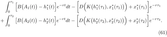
Z T
τ
B Aˆ(t)
e−rtdt−hDK h(τ), x(τ)
fires we will have prevention management following each fire event, but this is because we are essentially “resetting” our optimal control problem after every fire.
Let the value of the forest after the fire, withe−rτ factored out, be defined
by
J W τ, A(τ), h(τ), x(τ) =
Z T
τ
B Aˆ(t)
e−r(t−τ)dt−hDK h(τ), x(τ)
+x(τ)i.
(10)
Note that the ex post value of the forest is a function of the time of fire τ, the prevention management spendingh(τ), suppression spendingx(τ), and the number of unburned acres A(τ) at the time of fire, before the effects of the fire have been considered. We say that J W is a function of A(τ) and not
ˆ
A(τ) because ˆA is determined by the boundary condition containingA(τ) and the differential equation (6) with a dependence on K, the number of acres burned. Hence, given a time of fireτ, the corresponding prevention management spending at that timeh(τ), and the number of unburned acresA(τ) before the effects of the fire have been considered, the optimalex post value of the forest is the solution to
sup
x(τ) Z T
τ
B Aˆ(t)
e−r(t−τ)dt−hDK h(τ), x(τ)
+x(τ)i
subject tox(τ)≥0, (11)
where ˆA(t) = ¯A−
¯
A−A(τ)−K h(τ), x(τ)
x∗(τ) be the real-value scalar representing optimal suppression spending for a givenτ,h(τ), andA(τ), which maximizes the value of the forest after the fire. The maximized ex post value of the forest for a given τ, h(τ), and A(τ) is henceforth denoted by
J W∗ τ, A(τ), h(τ)
=J W τ, A(τ), h(τ), x∗(τ)
. (13) The value of the forest following a fire J W is maximized when evaluated at
x∗(τ). From our assumptions onD andK, we have that prevention spending increases the value of the forest following a fire:
∂J W∗ τ, A(τ), h(τ)
∂h >0. (14)
Once functional forms are chosen we explicitly determine x∗(τ), and thus
J W∗ τ, A(τ), h(τ)
, using scalar optimization techniques. The details surround-ing this process are discussed in Section 3.
2.2
Ex Ante
Fire Prevention
If the time of fireτ ∈[0, T] is strictly less than T, then the total value of the forest over the time horizon [0, T] is given by the sum of the net value of the forest before the fire and the net value of the forest after the fire up to timeT,
Z τ
0
B A(t)
−h(t)
e−rtdt+ Z T
τ
B Aˆ(t)
e−rtdt−hDK h(τ), x(τ)
+x(τ)ie−rτ,
If the time of the first fireτ is equal toT, then we represent the value of the forest over the time horizon [0, T] by
Z T
0 h
B A(t)
−h(t)ie−rtdt, (16) where A(t) is given by (3). In this case, we recognize that a fire will eventu-ally occur, but because it does not occur within the time horizon [0, T] we do not subtract the instantaneous suppression costs or cost of damages to built structures.
In summary, the value of the forest over [0, T] depends on the time of fire
τ, the prevention management spendingh, and the initial conditionA0=A(0) for the number of unburned acres in the forest before a fire. The value of the forest can thus be represented by the piecewise function
V(A0, τ, h) = Rτ 0 h
B A(t)
−h(t)ie−rtdt+e−rτJ W∗ τ, A(τ), h(τ)
ifτ < T
RT 0
h
B A(t)−h(t)ie−rtdt ifτ=T,
(17) whereA(t) is given by (3). Note that ˆA is completely contained withinJ W∗. The equationV(A0, τ, h) represents the net present value of the forest over the whole time interval [0, T] for a given time of fire τ, prevention management spendingh, and initial number of unburned acres in the forest A0. In the case that a fire happens within the time horizon, V incorporates the optimal value of the forest following a fireJ W∗ τ, A(τ), h(τ).
When the large fire event will occur is unknown. Thus, the time of fire
functionψ, defined as
ψ= lim ∆t→0
P r(fire in [t, t+ ∆t)
|no fire up tot) ∆t
. (18) The hazard function represents the conditional probability that a fire will occur at a timetgiven that no fire has occurred up to that time. Treating the hazard function as a function of time is consistent with the ecological concept of a fire return interval ([9]). For our problem, the hazard function is assumed to be a function of theex ante prevention management spending rate,
ψ=ψ h(t). (19) Furthermore, we assume that the hazard is decreasing with respect to an in-creased prevention management spending rate, i.e. ∂ψ∂h <0. A constant back-ground hazard is assumed in the absence of ex ante prevention management spending.
The survivor functionS(t), which gives the probability of the forest surviving to timetwith no fire, is related to the hazard functionψ in the following way:
S(t) =e−
Rt
0ψ h(z)
dz
. (20)
It follows thatS(0) = 1. While we assume that prevention spending can reduce hazard, we do not assume that prevention spending will indefinitely delay the occurrence of a large, stand-replacing fire. Therefore, we assume that the inte-gral representing the cumulative hazard,Rt
0ψ h(z)
dz, will diverge to positive
FT(τ) =
1−S(τ) ifτ < T
1 ifτ =T.
(21)
Notice the potential for discontinuity at time T. Hence, we observe that the probability density function forT ∈[0, T) is
fT(t) =ψ h(t)S(t). (22)
The mixed type RV T has a discrete component. For T =T, the probability mass is
P(T =T) =FT(T)−FT(T−) (23)
= 1− 1−S(T) =S(T).
Again, ifτ=T, no costs other than prevention management spendinghare considered. Our goal is to determine the prevention management spending rate
h(t) ≥0 which maximizes the net present value of the forest over [0, T] using deterministic optimal control. As written, our problem is currently stochastic. However, using techniques developed by Reed, we can convert this stochastic problem to deterministic by taking the expectation of (17) with respect to the RVT and introducing a state variable to represent cumulative hazard [31].
J(h) =ETV(A0, τ, h) =
Z T
0 "
Z τ
0 h
B A(t)−h(t)ie−rtdt+J W∗ τ, A(τ), h(τ)e−rτ
#
ψ h(τ)S(τ)dτ
+S(T) Z T
0 h
B A(t)
−h(t)ie−rtdt. (24)
After a bit of calculus, we arrive at
J(h) = Z T
0 h
B A(t)−h(t) +ψ h(t)J W∗ t, A(t), h(t)iS(t)e−rtdt. (25) This function,J(h), represents the expected net present value of the forest over an interval [0, T] subject to the survivor function S(t). By introducing a new state variable y to represent cumulative hazard we complete the conversion of our stochastic problem to deterministic. Letyrepresent cumulative hazard and be governed by the differential equation
y0(t) =ψ h(t)withy(0) = 0. (26) The initial conditiony(0) = 0 follows from the fact that S(0) = 1. Note that the survivor function can be rewritten as
S(t) =e−y(t), (27) and this allows us to rewrite (25) with our new state variabley.
be written as
sup
h∈U
Z T
0 h
B A(t)
−h(t) +ψ h(t)
J W∗ t, A(t), h(t)i
e−rt−y(t)dt (28) subject toy0(t) =ψ h(t)
withy(0) = 0, (29)
where
U =
h: [0, T]→[0,∞)|his Lebesgue measurable , (30) and
A(t) = ¯A−( ¯A−A0)e−δt. (31) Thus, our control problem with stochastic time of fire has been converted to a deterministic optimal control problem.
2.3
Linking Optimal Prevention and Suppression
Selecting explicit functional forms for B, K, D, and the hazard function al-lows us to determine the the optimal ex post value of the forest following a fire J W∗ τ, A(τ), h(τ) and ultimately solve our optimal control problem by determining the optimal management spendingh(t) rate over [0, T]. The ben-efits functionB represents the flow of benefits from the forest and is assumed directly proportional to the number of unburned acres in the forest:
B A(t)
=B1A(t), (32)
K(h, x) = k (k1+h)(k2+x)
, (33)
with parametersk > 0 andk1, k2 ≥1. The parameter kis related to the size of a fire. The parameterk1 controls the magnitude of the effect of prevention management spendinghon decreasing the number of acres burned. Similarly, the parameterk2 controls the magnitude of the effect of suppression spending
xon decreasing the number of acres burned. It is assumed that the cost of lost built structures is directly proportional to the number of acres destroyed in the fire:
D K(h, x)=cK(h, x) = ck (k1+h)(k2+x)
, (34)
with parameterc≥0 as the cost of damages in millions of dollars per thousand acres burned.
The hazard function ψ, representing the conditional probability that a fire will occur at timet given that a fire has not occurred up to that time:
ψ h(t)
=be−vh(t), (35)
is consistent with the literature [31, 27, 4, 7]. The parameter 0< b <1 repre-sents the constant hazard rate when there is no prevention management spend-ing. The constant v > 0 is used to control the effectiveness of preventative management spendingh(t) on reducing hazard.
max
x(τ) Z T
τ
B Aˆ(t)e−r(t−τ)dt−
DK h(τ), x(τ)+x(τ)
(36)
subject tox(τ)≥0,
where ˆA(t) = ¯A−
¯
A−A(τ)−K h(τ), x(τ)
e−δ(t−τ). (37) Using the solution to the state differential equation for ˆA(t) above, we integrate the flow of benefits from the time of fire τ to the end of our time horizon T. Hence, theex post value of the forest is given by
J W τ, A(τ), h(τ), x(τ) = B1
¯
A r
1−e−r(T−τ)
−B1
¯
A−A(τ)
δ+r
1−e−(δ+r)(T−τ)
−K h(τ), x(τ) B
1
δ+r
1−e−(δ+r)(T−τ)
+c
−x(τ). (38)
Our goal is to maximize J W τ, A(τ), h(τ), x(τ)
with respect to the one-time suppression costs x(τ). We do this using scalar optimization and thus consider the partial derivative ofJ W (38) with respect tox(τ). It follows that
x∗(τ) = 0 if ∂J W ∂x(τ)<0,
x∗(τ)≥0 if ∂J W ∂x(τ)= 0.
(39)
∂J W ∂x =−
B 1
δ+r
1−e−(δ+r)(T−τ)+c
∂K
∂x −1
= B
1
δ+r
1−e−(δ+r)(T−τ)+c
k
(k1+h)(k2+x)2
−1. (40)
If ∂x∂J W(τ) = 0, thenx∗(τ)≥0. To determinex∗(τ) in this case we set the partial derivative (40) equal to zero, and solve forx(τ). Asx(τ)≥0, we determine
0≤x∗(τ) =x∗ τ, h(τ)= s
k k1+h(τ)
B 1
δ+r
1−e−(δ+r)(T−τ)+c
−k2, (41) in the case that ∂x∂J W(τ)= 0.
If ∂x∂J W(τ) <0 andx∗(τ) = 0, then
s
k k1+h(τ)
B
1
δ+r
1−e−(δ+r)(T−τ)+c
−k2<0 =x∗(τ). (42)
Based on our choices for our functional forms, we see that optimal suppres-sion spendingx∗ is not only a function of the time of fire, but also prevention management spending h(τ). Note that maximum of J W could occur at the endpoint. Thus, it follows that optimal suppression spending is given by
x∗ τ, h(τ) = max
( 0,
s
k k1+h(τ)
B
1
δ+r
1−e−(δ+r)(T−τ)+c
−k2 )
.
J W∗ τ, A(τ), h(τ)=J Wτ, A(τ), h(τ), x∗ τ, h(τ). (44) We note that a quick calculation shows ∂2∂xJ W2 ≤0 and so theJ W value (41) is
indeed a maximum ofJ W (38).
We now work through the derivation of the conditional current-value opti-mality system. Let the standard Hamiltonian be given byH and let the adjoint function associated with state variable y by given by λ. Let the conditional current-value adjoint function be given by
ρ(t) =ert+y(t)λ(t). (45) The conditional current-value HamiltonianHis
H=ert+y(t)H (46)
=B A(t)−h(t) +ψ h(t)J W∗ t, A(t), h(t)+ρ(t)ψ h(t). (47) The partial derivative of the conditional current value Hamiltonian H with respect to the control is
∂H
∂h =−1 +J W
∗ t, A(t), h(t)∂ψ
∂h + ∂J W∗
∂h ψ h(t)
+ρ(t)∂ψ
∂h. (48)
ρ0(t) =r+ψ h(t)ert+y(t)λ(t) +ert+y(t)λ0(t) (49) =r+ψ h(t)
ρ(t)−ert+y(t)∂H
∂y (50)
Hence, the conditional current-value adjoint differential equation is
ρ0(t) =r+ψ h(t)ρ(t) +B A(t)−h(t) +ψ h(t)J W∗ t, A(t), h(t), (51) with transversality condition
ρ(T) =erT+y(T)λ(T) = 0. (52) The hazard functionψis nonlinear inh, as is the functionJ W∗ t, A(t), h(t)
, which represents the optimal value of the forest following a forest fire for a given time of fire and a given amount of prevention management spending at the time of fire. We utilize the fact that Pontryagin’s Maximum Principle (PMP) states that the optimal control maximizes the Hamiltonian with respect to the control
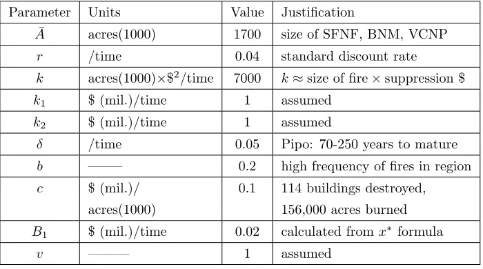
Table 1: The table below includes the parameter values chosen to reflect the 2011 Las Conchas Fire.
Parameter Units Value Justification
¯
A acres(1000) 1700 size of SFNF, BNM, VCNP
r /time 0.04 standard discount rate
k acres(1000)×$2/time 7000 k≈size of fire×suppression $
k1 $ (mil.)/time 1 assumed
k2 $ (mil.)/time 1 assumed
δ /time 0.05 Pipo: 70-250 years to mature
b ——– 0.2 high frequency of fires in region
c $ (mil.)/ 0.1 114 buildings destroyed,
acres(1000) 156,000 acres burned
B1 $ (mil.)/time 0.02 calculated fromx∗ formula
v ——— 1 assumed
∂2H
∂h2 ≤0, (53)
numerically for our given functions and parameter choices. An iterative method is used to
3
Las Conchas Fire: Numerical Example
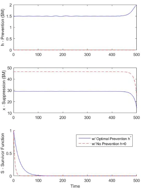
Figure 1: The plots above contain the h∗, x∗, and S results of our optimal control problem using the Las Conchas Fire parameter set. For comparison, in each plot we include the case with optimal prevention management spendingh∗
acres burned in the fire and over $40 million were spent on fire suppression efforts [25, 36, 42]. In addition to suppression costs, over 110 structures were destroyed or damaged during the fire [25, 36]. We are using the data from this fire to build a more realistic problem, not to draw any retrospective conclusions concerning prevention management or suppression spending decisions made at the time of this fire. Parameter choices are summarized in Table 1.
The parameter ¯A represents the “size of the forest” in units of thousands of acres. The Las Conchas Fire mainly burned through the Santa Fe National Forest, Bandelier National Monument, and Valles Caldera National Preserve and the combined size of these three areas is approximately 1,722 thousand acres[24, 41, 44]. Rounding down, we take ¯A= 1,700.
The parameter δ represents the regeneration rate of the forest following a fire. We chooseδ based on the dominant tree type in the forest, which in the Santa Fe National Forest is Ponderosa Pine (Pipo). The age of Ponderosa Pine at maturity is 70-250 years [40]. Assuming that at the time of fire the number of unburned acres is reduced by half, we choose a value forδso that the number of unburned acres after 100 years has approximately returned to ¯A. As such, we choose δ = 0.05. The discount rate is set at 4 percent in accordance with USDA Forest Service practice: r = 0.04 [32]. The parameter b, found in the hazard functionψ h(t), represents the background fire hazard. To capture the probability that large, high-severity fires happen frequently in the region, we choose b = 0.2 [45]. For b = 0.2 the probability of the forest surviving to 3.5 years with no fire is approximately 0.5.
the number of acres that will be completely burned in the fire given that there is no prevention management spending or suppression spending at the time of the fire. In particular, given that we know the number of acres burned in the Las Conchas Fire and the amount spent on suppression, we use the functionK
to estimate a value for the fire severity parameterk. Assuming that there is no prevention management spending at the time of fire, we havek≈K×(1 +x), whereKrepresents the number of acres burned (in thousands) in the fire andx
represents the amount spent on suppression (in millions). For the Las Conchas Fire, approximately 157 thousand acres were burned and over $40M were spent on suppression. Thus, we choosek= 7,000 given that estimates for suppression costs range between $40M and $50M.
The parameter v is found in the hazard function ψ and represents the ef-fectiveness of prevention management spending on reducing hazard. From the literature, we choosev= 1 [28, 4].
The parametercrepresents the cost of damages to built structures in millions of dollars per thousand acres burned. In the Las Conchas Fire, 114 buildings were destroyed or damaged in the fire [36]. The median value of homes in the region ranges between $100,000 and $450,000 [39]. First, we estimate the cost of non-timber damagesDfor the Las Conchas Fire by multiplying the number of building destroyed by the median value of homes in the area. Our estimate forD is thus $17.2 million. We then divide this estimate forD by the number of acres destroyed in the fire,K= 157, to estimate an appropriate value for c;
c≈ D
K. For the Las Conchas Fire in particular, we round and takec= 0.1.
for optimal suppression spending (41) to determine a value for B1 based on our other parameter choices and the amount of money spent on suppression for the Las Conchas Fire. In order to determine a reasonable estimate for
B1, we assume that the amount of suppression spending was optimal and we allow this amount to stand in forx∗. We then solve equation (41) for B1 and approximate its value using our previous parameter choices. Furthermore, we assumeh(τ) = 0, τ = 0, andT = 500.This leads to the choice ofB1= 0.02 for the Las Conchas Fire.
We recognize that the selection of some of these parameter values is not literature driven. Because of this, we perform a sensitivity analysis to determine which parameters have the most impact on the overall expected net present value of the forest. We use Latin Hypercube Sampling (LHS) and Partial Rank Correlation Coefficient (PRCC) analysis to determine the parameters to which the value of the objective functional evaluated at the optimal controlh∗is most
sensitive. Ten parameters with appropriate ranges were chosen for this analysis and the full details are shown in the appendix. We conclude that the parameter
B1 has the strongest impact on the expected net present value of the forest
J(h∗), followed by parameters ¯A and r, followed by parametersc andk2. We note that using the objective functional at the optimal control as an output for a LHS/PRCC analysis is novel.
our consideration of sequences of fires.
From our numerical results in Figure 1, the optimal prevention management spending rateh∗ is approximately constant at 1.5 million dollars per year over the course of the time horizon, with an increase to 2 million near the end of the time horizon. This increase is likely due to the sharp decrease in the value of J W∗ near the end of the time horizon. Hence, we interpret the graph of
h∗ as saying that approximately $1.5 million should be spent on prevention management per year, up to the time of the first fire, which in practice is unknown.
Recall that the fire event in our problem is taken to be instantaneous, along with its associated costs. As seen in Figure 1, the function representing optimal suppression spending in the optimal prevention management spending case is approximately constant at $29M over the time horizon, except for effects at the end. It is important to recall that suppression spending is a one-time instanta-neous cost at the time of the fire and therefore, the suppression cost of $29M only occurs once in application at the time of fire. This is in contrast to the optimal prevention management spending h∗, discussed in the previous para-graph, which is ongoing up to the time of fire. In the case without prevention management spending, instantaneous suppression spending is roughly $46.5M at the time of fire, given that the function forx∗in the case without prevention management spending is approximately constant over the course of the time horizon. As expected, instantaneous suppression spending in the case with-out prevention management spending is greater than instantaneous suppression spending in the optimal prevention case: ∂x∗
∂h < 0. Moreover, instantaneous
Given that the time of fire is treated as a random variable in our problem, we would like to compare the expected time of the next fire between the two cases of optimal prevention management and no prevention management. In order to determine this value, we calculate the expected value of the time of fire random variable. The expected value of the time of fire random variable is justifiably approximated by
E[T] = Z T
0
tψ h(t)
e−y(t)dt. (54) In the case of no prevention management spending, this is reduced to
Z T
0
bte−btdt. (55) The mean time of fire in the case without prevention management spending is 5 years. In the case of optimal prevention management spending, the mean time of fire is approximately 22.3 years. Hence, on average, the time of the fire in the optimal case is approximately 17 years later than the no prevention case. Furthermore, in the case of multiple fires, we might expect that over a fixed amount of time there will be fewer fires when optimal prevention management spending is employed compared to when there is no prevention management spending.
Another measure we wish to consider is the expected net present value of the forest over [0, T]. This is given by the value of the objective functional in our optimal control problem, either evaluated at the optimal controlh∗ or
management spending is applied.
Overall, we see that in the case of optimal prevention management spending
h∗, the value of the forest, and the mean time of fire are larger than in the case without prevention management spending,h= 0. However, we recognize that it is unrealistic to assume that only one fire will occur in 500 years, especially since we chose the background hazard b to reflect a high frequency of fires in the region. Thus, in order to make better comparisons concerning the value of the forest and the trade-offs between prevention management and suppression spending, we would like to apply our optimal control problem to a sequence of fires over a fixed amount of time in Section 4.
4
Applying Optimal Prevention Strategies to a
Sequence of Fires
Our goal is to explore the effects of prevention management spending on the value of a forest over a fixed number of years given that a sequence of an unknown number of large fire events may occur within this time. Let this fixed management horizon that we wish to consider a sequence of fires over beY years long.
We are optimizing prevention management spending between each fire event using our optimal control problem. We determine JY, the value of the
for-est over Y years, and consider the trade-offs in total prevention management spending and suppression spending. Because we are sampling the times of the fires, each time we determine JY years will be different. Thus, we perform a
suppression spending overY years. For comparison, we also consider the case without prevention management spending.
4.1
Fire Sequence Simulation
As our optimal control problem allows for non-constant unburned acres before a fire, it possible to consider sequences of fires. In essence, we solve our optimal control problem, usey∗to build the CDF of RVT, sample for a time of fire, and then solve our optimal control problem again with an updated initial condition
A0 for the number of unburned acres in the forest. This new initial condition takes into account the number of acres destroyed in the fire according to the previous solution of the optimal control problem. We continue to do this until the time of thenthfire,nunknown, is beyond a specified amount of time, Y.
The parameterY represents the the length of the management horizon over which we want to consider a sequence of fires. Over the course of the manage-ment horizon [0, Y], our optimal control problem will be solved several times. Each time the optimal control problem is solved over the time horizon [0, T]. After a fire event, the time of the next sampled fire time τ is in [0, T]. The length of the time horizon for our optimal control problemT should be chosen so thatS(T) is very small (close to zero) so that we can approximate the CDF forT by its continuous counterpart.
Here, we explain the process used for a single simulation of a sequence of fires. Within a single simulation, or trial, we solve our optimal control problem multiple times and as such we will need to distinguish between the different state and control variables corresponding to the different solutions for the optimal control problem. To do this, we use numerical subscripts to indicate which solution to which the variables correspond.
initial conditionA1(0) = ¯A. As a result, we know the optimal prevention man-agement spendingh∗1(t), the optimal instantaneous suppression spendingx∗1(t), the optimal cumulative hazardy∗1(t), and the number of unburned acresA1(t) over the time horizon [0, T]. Note the subscript 1 on the variables denotes that these functions correspond to the solution of our first optimal control problem. The number of unburned acres A1(t) is unaffected by either control variables
xandh and as such, we do not use the star notation with it; it is completely determined by (3). After numerically determining the solution, we build the CDF for the time of fire RVT usingy∗ and sample for the time of the first fire. Letτ1∈[0, T] be the sampled time of the first fire. Ifτ1> Y, then the value of the forest, denoted byJY, overY years is given by
JY =
Z Y
0 h
B A1(t)−h∗1(t) i
e−rtdt, (56) We do not consider costs of suppression or non-timber damages because the time of the first fire is outside of our management horizonY. If τ1 =Y, then the value of the forest up to timeτ1=Y is given by
JY =
Z Y
0 h
B A1(t)
−h∗1(t)ie−rtdt−
DK h∗1(τ1), x∗1(τ1)
+x∗1(τ1)
e−rτ1,
(57) Here, we consider the cost of suppression and cost to built structures because the time of the first fire occurs at the end of the management horizon Y. If
τ1< Y, then value of the forest up to timeτ1 is given by
Z τ1
0 h
B A1(t)
−h∗1(t)ie−rtdt−
DK h∗1(τ1), x∗1(τ1)
+x∗1(τ1)
and we need to solve our optimal control problem again and sample for the time of the next fire since τ1 < Y. The expression directly above is not labeled as
JY because we have not yet accounted for the whole management horizon.
Now that a fire has occurred, and τ1 < Y, the number of unburned acres is less than ¯A and we need to set the initial conditionA2(0) to prepare for the next application of our optimal control problem. In particular, we set our new initial condition to be
A2(0) =A1(τ)−K h∗1(τ1), x∗1(τ1)
, (59)
where A1(τ) = ¯A. Note that A1(τ) = ¯A because for our first solution of our optimal control problem we chose the initial condition forAto be at an equi-librium point. We point out again that while this initial condition is dependent on prevention management spending and suppression spending, it is from the previous optimal control solution, and thus completely known.
After each fire event, we are in essence “resetting” our problem. With our new initial condition, we solve our optimal control problem using the same set of parameters over [0, T] and once again, as a result, we will knowh∗2(t),x∗2(t), andy2∗(t) over the time horizon [0, T]. Thus, as before, we sample for the time of the second fire,τ2, using the CDF constructed using y∗2. Thus, the time of the second fire in the context of our management horizon [0, Y] isτ1+τ2, the sum of the first sampled time of fire and the second sampled time of fire.
Ifτ1+τ2> Y, then the value of the forest overY years is given by
JY =
Z τ1
0 h
B A1(t)
−h∗1(t)ie−rtdt−
DK h∗1(τ1), x∗1(τ1)
+x∗1(τ1)
e−rτ1
+ Z Y−τ1
0 h
B A2(t)
Here, we take into account the cost associated with the first fire because it falls within [0, Y]. We do not take into account the costs associated with the second fire because becauseτ1+τ2> Y. Also notice that the limits of integration for the second integral are from 0 toY −τ1. We begin at the time t= 0 because the optimal control problem is solved over [0, T]. We only integrate up toY−τ1 because there are onlyY −τ1years from the time of the first fireτ1to the end of the management horizonY.
Ifτ1+τ2≤Y, then the value of the forest up toτ1+τ2 years is given by
Z τ1
0 h
B A1(t)−h∗1(t)ie−rtdt−
DK h∗1(τ1), x∗1(τ1)+x∗1(τ1)
e−rτ1
+ Z τ2
0
B A2(t)−h∗2(t) i
e−rtdt−
DK h∗2(τ2), x∗2(τ2)
+x∗2(τ2)
e−rτ2.
(61)
Ifτ1+τ2 =Y, we are done since τ2 =Y −τ1. However, if τ1+τ2 < Y, once again, we must sample for another time of fire and solve our problem again. We set our new initial condition for unburned acres,
A3(0) =A2(τ2)−K h2∗(τ2), x∗2(τ2)
, (62)
solve our optimal control problem, and sample the next time of fire. We continue to do this until the sum of the sampled fire times is greater than or equal toY:
τ1+τ2+· · ·+τn≥Y.
Figure 2: The top plot gives management prevention spending with optimal prevention and without prevention over a management horizonY = 50 years The bottom plot gives the number of unburned acres. Every jump discontinuity represents a fire event.
The only difference is that we choose a smaller value for the background hazard
band we letb= 0.1. These plots also show what the number of unburned acres might look like given no prevention management spending. This simulation is determined separately from the optimal case. This is becauseh determinesy
which is used to build the CDF used for sampling a time of fire. The jump dis-continuities in the plots correspond to the different fire events. In the particular example in Figure 2 the no prevention management spending case 5 fires occur in 50 years and in the optimal prevention case 2 fires occur.
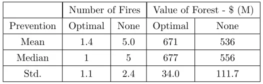
Number of Fires Value of Forest - $ (M) Prevention Optimal None Optimal None
Mean 1.4 5.0 671 536
Median 1 5 677 556
Std. 1.1 2.4 34.0 111.7
Table 2: This table provides statistics concerning the average number of fires and average value of the forest over 50 years for 500 simulations.
large value forTand the initial conditionA1(0). The initial conditionA1(0) = ¯A
only holds for the first solution of the optimal control problem in a single trial. Following that, the initial condition for the number of unburned acres following the first fire in a single trial are determined based on the sampled time of fire.
For the simulation study, 500 trials are conducted to determine the value of the forestJY over 50 years, given that an unknown number fires may occur
in this time period for each trial. In addition to calculating value of the forest
JY using the prevention management schedule found according to the optimal
control problems, for comparison, we also calculate the value of the forest given that no money is spent on prevention management. It is important to note that these two cases are determined independently from one another. We also consider total prevention management spending and suppression spending in each case, in addition to the number of fires that occur in the management horizon. The results from the simulation study are discussed below.
of the number of fires is approximately 1 in the optimal prevention management case and greater than 2 in the no prevention management case. Moving from a case where there is no spending on prevention management to the case with optimal prevention management shown here, there is on average a 72% reduction in the number of fires that occur within 50 years. Hence, applying optimal prevention management spending reduces the risk of fire for a forest.
Additionally, Table 2 provide details concerning the distribution of the value of the forestJY over 50 years across 500 simulations. In the optimal prevention
case the mean value of the forest over 50 years is $671 million dollars and in the case without prevention management the mean value of the forest over 50 years is $536 million dollars. Additionally, the standard deviation of the distribution for the value of the forest in the optimal prevention management case is 34.0, compared to 111.7 in the no prevention management case. That is, the stan-dard deviation is three times larger in the case without prevention management spending compared to the case with optimal prevention management. Hence, the value of the forest over 50 years with multiple fires, is less variable and on average adds a value of $1.2M per year to the value of the forest in the case of optimal prevention management compared to the case without prevention management.
the potential to offset high suppression costs and decrease spending overall. Our results reveal that, on average, in the case of optimal prevention man-agement spending there are fewer fires and an increased value of the forest in comparison to the case with no prevention management spending. Furthermore, the standard deviation around the average number of fires and value of the forest is much smaller in the optimal prevention management case in comparison to the no prevention management case. This suggests that using optimal preven-tion management spending is a less risky management oppreven-tion when compared to the case without prevention management spending. Additionally, we see that prevention management spending can offset high suppression costs and decrease the total amount of spending overall.
5
Conclusions
spending over a finite management horizon given an unknown sequence of fires. We find that with the application of preventive fuel management, the value of the forest is greater and less variable than in the case where prevention management spending is not applied to the forest. We also find that prevention spending lowers the number of devastating large fire events. The mean value of the forest over a 50 year time horizon in the no prevention management case is $536M with a standard deviation of $111.7M. When prevention is determined by the successive application of our optimal control problem, we find that the mean value of the forest over 50 years to be $671M with a standard deviation of $34.0M.This result illustrates that there are real economic costs associated with using funding for fuel management to fund immediate fire suppression.
Perhaps more surprisingly, we find that when optimal prevention manage-ment is employed, not only are high suppression costs drastically reduced, total spending on fire management (prevention and fire suppression) is less than the case without prevention management. In the case without prevention manage-ment spending, $236M was spent on average on fire suppression over the course of 50 years. In the case with applying optimal prevention management spend-ing, only $42M was spent on average on suppression over 50 years and $65M was spent on prevention management. By comparison, $40M-$50M was spent fight-ing the Las Conchas fire. In our work with unknown fire sequences, we observed an 88% reduction in suppression spending on average with prevention manage-ment, and a 55% reduction in spending overall. This result provides hope that a more careful integration of fire prevention into wildfire management plans may actually reduce the cost of these plans.
preven-tion (mechanical thinning, prescribed fire) decays rapidly. There is very little data on the longevity of fire prevention expenditures. In forests that regenerate slowly, the effect of prevention expenditures may last for many years. In forests that regenerate rapidly, the effect of prevention may be short-lived. But how long prevention lasts will also vary by the type of prevention. For instance, the effects of prescribed fire may be temporary in forests that regenerate through fire. Thus, identifying how long the effect of fire prevention expenditures should last is complicated. Since our results tend to highlight the value of prevention, we elected to adopt a conservative assumption that would work lower the value of prevention. Thus our results can be viewed as a lower bound estimate of the value of prevention relative to suppression.
In spite of our results, expenditures on fire suppression will likely continue to outweigh hazardous fuel reduction expenditures. There are a number of fac-tors not considered in our model that may explain this paradox. In our model, forest managers are forward-looking when they select suppression expenditures. However, forest managers acknowledge that public outcry during a large fire of-ten prevents them from saving resources to fight future fires. To date, Congress has made up for any budget shortfalls that occur due to unexpected fire sup-pression expenditures. These factors suggest that forest mangers may choose fire suppression expenditures more myopically than our model suggests. These political economy considerations could be investigated by allowing theex ante
and ex post problems to be solved for different planning horizons. There are also additional liability considerations associated with prevention activities such as prescribed burning that our model does not consider. We leave these issues for future work.
additional stochastic feature due to modeling a variety of types of fires would be interesting to pursue in the future. We also note that investigating models with explicit spatial components would be worthwhile in the future.
Acknowledgments: This work was partially supported by the National Insti-tute for Mathematical and Biological Synthesis, an InstiInsti-tute sponsored by the National Science Foundation through NSF Award DBI-1300426, with additional support from The University of Tennessee, Knoxville. Sims gratefully acknowl-edges funding from USDA Forest Service Grant No. 16-JV-11221636-104.
References
[1] Abdi, H. (2007). Bonferroni and ˇSid´ak corrections for multiple comparisons.
Encyclopedia of Measurement and Statistics, 3:103–107.
[2] Agee, J. K. and Skinner, C. N. (2005). Basic principles of forest fuel reduc-tion treatments. Forest Ecology and Management, 211(1):83–96.
[3] Anderson, T. (1984). Multivariate statistical analysis.Wiley and Sons, New York, NY.
[4] Berry, K., Finnoff, D., Horan, R. D., and Shogren, J. F. (2015). Managing the endogenous risk of disease outbreaks with non-constant background risk.
Journal of Economic Dynamics and Control, 51:166–179.
[5] Calkin, D. E., Gebert, K. M., Jones, J. G., and Neilson, R. P. (2005). Forest service large fire area burned and suppression expenditure trends, 1970–2002.
Journal of Forestry, 103(4):179–183.
[7] Finoff, D., Shogren, J. F., Leung, B., and Lodge, D. (2007). Take a risk: pre-ferring prevention over control of biological invaders. Ecological Economics, 62(2):216–222.
[8] Gebert, K. M. and Black, A. E. (2012). Effect of suppression strategies on federal wildland fire expenditures. Journal of Forestry, 110(2):65–73.
[9] Grissino-Mayer, H. D. (1999). Modeling fire interval data from the amer-ican southwest with the weibull distritbution. Environmental Modelling & Software, 9.1:37–50.
[10] Hessburg, P. F., Agee, J. K., and Franklin, J. F. (2005). Dry forests and wildland fires of the inland northwest usa: contrasting the landscape ecology of the pre-settlement and modern eras. Forest Ecology and Management, 211(1):117–139.
[11] Hesseln, H. (2000). The economics of prescribed burning: a research review.
Forest Science, 46(3):322–334.
[12] Holmes, T. P., Prestemon, J. P., and Abt, K. L. (2008). The economics of forest disturbances: Wildfires, storms, and invasive species, volume 79. Springer Science & Business Media.
[13] Horan, R. D. and Fenichel, E. P. (2007). Economics and ecology of man-aging emerging infectious animal diseases. American Journal of Agricultural Economics, 89(5):1232–1238.
[14] Iman, R. L. and Helton, J. C. (1988). An investigation of uncertainty and sensitivity analysis techniques for computer models. Risk Analysis, 8(1):71– 90.
[16] Lenhart, S. and Workman, J. T. (2007). Optimal Control Applied to Bio-logical Models. Chapman & Hall/CRC.
[17] Marino, S., Hogue, I. B., Ray, C. J., and Kirschner, D. E. (2008). A methodology for performing global uncertainty and sensitivity analysis in systems biology. Journal of Theoretical Biology, 254(1):178–196.
[18] McKay, M. D., Beckman, R. J., and Conover, W. J. (2000). A comparison of three methods for selecting values of input variables in the analysis of output from a computer code. Technometrics, 42(1):55–61.
[19] Mercer, D. E., Haight, R. G., and Prestemon, J. P. (2008). Analyzing trade-offs between fuels management, suppression, and damages from wildfire. In
The Economics of Forest Disturbances, volume 1, pages 247–272. Springer.
[20] Mercer, D. E., Prestemon, J. P., Butry, D. T., and Pye, J. M. (2007). Evalu-ating alternative prescribed burning policies to reduce net economic damages from wildfire. American Journal of Agricultural Economics, 89(1):63–77.
[21] Milne, M., Clayton, H., Dovers, S., and Cary, G. J. (2014). Evaluating benefits and costs of wildland fires: critical review and future applications.
Environmental Hazards, 13(2):114–132.
[22] Minas, J., Hearne, J., and Martell, D. (2015). An integrated optimiza-tion model for fuel management and fire suppression preparedness planning.
Annals of Operations Research, 232(1):201–215.
[23] National Interagency Fire Center (2016). NIFC Fire Information: Statis-tics. https://www.nifc.gov/fireInfo/fireInfo_statistics.html.
[24] National Parks Service (2017). Bandelier National Monument. https:
[25] National Wildfire Coordinating Group (2013). Inciweb: Incident Informa-tion System: Las Conchas. https://inciweb.nwcg.gov/incident/2385.
[26] Ninan, K. and Inoue, M. (2013). Valuing forest ecosystem services: what we know and what we don’t. Ecological Economics, 93:137–149.
[27] Reed, W. J. (1984). The effects of the risk of fire on the optimal rotation of a forest. Journal of Environmental Economics and Management, 11:180–190.
[28] Reed, W. J. (1987). Protecting a forest against fire: Optimal protection patterns and harvest policies. Natural Resource Modeling, 2:23–54.
[29] Reed, W. J. (1988). Optimal harvesting of a fishery subject to random catastrophic collapse. Mathematical Medicine and Biology, 5(3):215–235.
[30] Reed, W. J. and Apaloo, J. (1991). Evaluating the effects of risk on the economics of juvenile spacing and commercial thinning. Canadian Journal of Forest Research, 21(9):1390–1400.
[31] Reed, W. J. and Heras, H. E. (1992). The conservation and exploitation of vulnerable resources. Bulletin of Mathematical Biology, 54(2/3):185–207.
[32] Row, C., Kaiser, H., and Sessions, J. (1981). Discount rate for long-term forest service. Journal of Forestry, 79(6):367–369.
[33] Rummer, B., Prestemon, J., May, D., Miles, P., Vissage, J., McRoberts, R., Liknes, G., Shepperd, W. D., Ferguson, D., Elliot, W., et al. (2005). A strategic assessment of forest biomass and fuel reduction treatments in western states. https://pdfs.semanticscholar.org/eabf/
2f388d6e6202f6826f6341c1aa9d25254ac2.pdf.
[35] Service, N. P. (2016). Wildland fire strategic planning. https://www.nps.
gov/fire/wildland-fire/about/plans.cfm.
[36] Southwest Fire Science Consortium (2011). Las Conchas Fire: Jemez Mountains, NM. http://swfireconsortium.org/wp-content/uploads/
2012/11/Las-Conchas-Factsheet_bsw.pdf.
[37] Stephens, S. L. and Ruth, L. W. (2005). Federal forest-fire policy in the united states. Ecological applications, 15(2):532–542.
[38] Thompson, M., Anderson, N., et al. (2015). Modeling fuel treatment im-pacts on fire suppression cost savings: A review. California Agriculture, 69(3):164–170.
[39] Trulia, Inc. (2017). Trulia. https://www.trulia.com.
[40] United States Department of Agriculture (2002). Plant Fact Sheet: Pon-derosa Pine. https://plants.usda.gov/factsheet/pdf/fs_pipo.pdf.
[41] United States Department of Agriculture: Forest Service (2007). NFS Acreage by State, Congressional District and County.https://www.fs.fed.
us/land/staff/lar/2007/TABLE_6.htm.
[42] United States Department of Agriculture: Forest Service (2011). Southwest Jemez–CFLRP Annual Report 2011. https://www.fs.usda.gov/detail/
santafe/landmanagement/projects/?cid=stelprdb5416651.
[43] United States Department of Agriculture: Forest Service (2015). Land Areas of the National Forest System.http://studylib.net/doc/10421337/
land-areas-of-the-national-forest-system.
[45] United States Department of Agriculture: Forest Service (2017b). Santa Fe National Forest GIS Data. https://www.fs.usda.gov/detail/r3/
landmanagement/gis/?cid=stelprdb5203736.
A
Appendix: Global Parameter Sensitivity
Anal-ysis
The values chosen for our parameters are not all strictly data driven or from literature sources. Thus, we perform a global sensitivity analysis to determine which parameters have the most significant impact on the expected value of the forest, J(h∗) [14, 17]. We use Latin Hypercube Sampling (LHS) and Partial Rank Correlation Coefficient (PRCC) analysis to determine the parameters to which the value of the objective functional evaluated at the optimal controlh∗
is most sensitive.
LHS was introduced in 1979 by M.D. McKay as an improved alternative to simple random sampling in Monte Carlo studies[18]. The LHS method provides similar accuracy as simple random sampling methods, but with fewer iterations, making it particularly useful for computationally expensive models [14, 17, 18]. There are 10 parameters in our optimal control problem that we will investi-gate. They are listed in the first column of Table 3. First, we must determine an appropriate range over which to investigate each of the parameters, or “inputs”. For each parameter we must choose an appropriate lower and upper bound for the parameter range; see Table 3. Next, we briefly discuss how these ranges were chosen. We note that while the values for the parameters chosen for the Las Conchas Fire example are included in these ranges, they do not serve as the baseline values for the parameters.
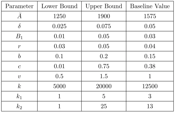
Table 3: The table below contains the lower and upper bounds of the parameter values to be used in our LHS/PRCC analysis. The baseline value for a given parameter is simply the average of the lower and upper bounds.
Parameter Lower Bound Upper Bound Baseline Value ¯
A 1250 1900 1575
δ 0.025 0.075 0.05
B1 0.01 0.05 0.03
r 0.03 0.05 0.04
b 0.1 0.2 0.15
c 0.01 0.75 0.38
v 0.5 1.5 1
k 5000 20000 12500
k1 1 5 3
k2 1 25 13
forests in the United States and is given in thousands of acres [43]. The forest regeneration rateδ parameter range is centered around our original choice of
δ = 0.05 for Ponderosa Pine in the previous fire examples. Recall that for a particular fire event we determine a value for the flow of benefits parameter
be smaller than the range for parameterk2 because, at a given point in time, less is spent on prevention management than on suppression. The choice for the background hazard parameter b was chosen to reflect the frequency with which large fire events may occur in a given area. The range for the discount rate parameterr is centered and varied around our original choice ofr= 0.04. The range for the prevention management effectiveness parameterv, found in the hazard function, is centered and varied around our original choice ofv= 1. In order to properly use LHS, we must first verify that the output in question,
J(h∗), is monotonic with respect to each parameter[18]. That is, we solve our optimal control problem multiple times across the range of a given parameter, with all other parameters held at their baseline values, which is simply the average of the lower and upper bound for that parameter. We then verify that the value of the objective functional evaluated at the optimal control h∗ is monotonic with respect to changes in the parameter. We repeated this process for every parameter and verified the monotonicity.
The LHS parameter matrix can now be generated. The LHS matrix is an
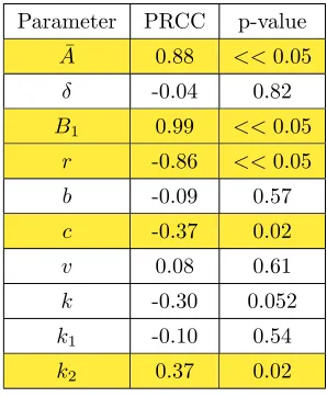
Table 4: In this table, the partial rank correlation coefficients for each param-eter associated with the outputJ(h∗), along with the corresponding p-values, are listed. Using a significance level ofα= 0.05 we see that 5 of the 10 param-eters investigated are significantly different from zero. They are highlighted in yellow.
Parameter PRCC p-value ¯
A 0.88 <<0.05
δ -0.04 0.82
B1 0.99 <<0.05
r -0.86 <<0.05
b -0.09 0.57
c -0.37 0.02
v 0.08 0.61
k -0.30 0.052
k1 -0.10 0.54
k2 0.37 0.02
Once the LHS matrix has been generated we solve our optimal control prob-lem 50 times, once for each row vector of parameter values from the LHS ma-trix. For each trial,J(h∗) is calculated. The mean ofJ(h∗) for the 50 trials is
µ= $1,153M. Given that the standard deviation for the output, σ= $525M, is large in comparison to the mean, it is clear that the uncertainty present in the value ofJ(h∗) is substantial. That is, variation in our choice of parameter values has a significant impact on J(h∗). Hence, we follow this work with a PRCC sensitivity analysis to determine which parameters are the most signifi-cant contributors to this uncertainty.
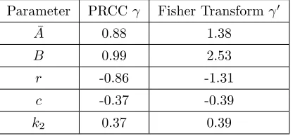
Table 5: This table lists the PRCCs and their corresponding Fisher transforms for the parameters which were shown to have the most impact on the value of the objective functional evaluated at the optimal controlh∗.
Parameter PRCCγ Fisher Transformγ0
¯
A 0.88 1.38
B 0.99 2.53
r -0.86 -1.31
c -0.37 -0.39
k2 0.37 0.39
The PRCC for each parameter and associated p-values in Table 4 are cal-culated using the MATLAB functionpartialcorr(). The p-values are used to assess whether or not the PRCCs are significantly different from zero. Using a significance level ofα= 0.05, we see that 5 of our 10 parameters have PRCCs significantly different from zero. These parameters include the size of the forest parameter ¯A, the flow of benefits parameterB1, the discount rate parameterr, the nontimber damage cost parameterc, and the suppression spending effective-ness parameterk2. We interpret this to mean that the parameters which have PRCCs significantly different from zero have a significant impact onJ(h∗).
Now that we know which parameters have a significant impact on the output, we would like to make a comparison of these significant parameters to see which ones have the strongest impact, in magnitude, onJ(h∗). To determine if a given parameter has a greater impact on the output than another, we must determine if there are significant statistical differences in their corresponding PRCCs. In order to perform statistical comparison tests for PRCCs, we must first apply the following log transformation to each PRCC:
γ0 =1 2ln
1 +γ
1−γ
, (63)
transformed PRCC γ0 is known as the Fisher tranform and is approximately GaussianN(µ, σ2) with
µ= 1 2ln
1 +γ
1−γ
andσ2= 1
N−3−p, (64)
whereN is the number of trials andp is the number of parameters controlled for when the PRCC is calculated. Table 5 gives the Fisher transformed PRCCs for the parameters whose PRCCs are significantly different from zero.
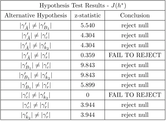
We can compare the values of two PRCCs by examining the z-statistic
z= γ
0
1−γ20 q
1
N1−3−p1+
1 2−3−p2
, (65)
which follows a N(0,1) distribution. Here, N1 = N2 = 50 is the number of trials and the valuepi,i= 1,2, represents the number of parameters controlled
for when the PRCCγiis calculated [17]. For our problem,p1=p2= 9 since we are investigating 10 parameters. We are most interested in determining which parameters have the largest impact on the output in magnitude, regardless of whether that impact is positive or negative. This guides the development of the family of hypotheses we wish test to determine the ranking of the significant parameters.
To properly rank the PRCCs according to their impact on the outputJ(h∗)
in magnitude, we must perform multiple pairwise comparison tests. In particu-lar, we test the null hypothesis that all PRCCs are equal
H0:|γA0¯|=|γB01|=|γ
0
c|=|γ
0
k2|=|γ
0
r| (66)
against the alternative hypotheses
for every pair (i, j)∈ {A, B¯ 1, c, k2, r} where i6=j. Thus, we have a family of 5
2
= 10 pairwise hypothesis tests to perform in order to effectively rank our 5 significant parameters.
When performing multiple comparison tests we must be careful to consider the increased likelihood of a rare event; that is, when considering multiple tests, we are more likely to reject the null hypothesis when it is true, a type I error. Given that we are performing 10 hypothesis tests and have chosen a significance level ofα= 0.05, the probability that we reject at least one of the null hypotheses (i.e. the probability of at least one rare event) is
P(≥1 significant event) = 1−P(0 significant events) = 1−(1−0.05)10
= 0.40126. (68)
In other words, using a significance level ofα= 0.05 for each of the 10 tests, the probability of at least one significant event (at least one rejection of the null hypothesis) is approximately 40%. This is known as the familywise error rate (FWER). We would like to control the FWER on our family of hypothesis tests in order to control the number of false positives. To do so, we need to differentiate between a per test significance levelα[P T], read “alpha per test,” and a per family significance level α[P F], read “alpha per family.” Given a family of hypothesis tests we would like to control the familywise error rate at the level ofα[P F] = 0.05. The FWER for a givenα[P T] is given by