The Definite Integral

262

Chapter

T

he 1995 Reader’s Digest Sweepstakes grand prize winner is being paid a total of $5,010,000 over 30 years. If invested, the winnings plus the interest earned generate an amount defined by:

AerT

T 0

mPert_dt

(rinterest rate, Psize of payment, Tterm in years, mnumber of payments per year.)

Would the prize have a different value if it were paid in 15 annual installments of $334,000 instead of 30 annual installments of $167,000? Section 5.4 can help you compare the total amounts.

The Definite

Integral

Chapter 5 Overview

The need to calculate instantaneous rates of change led the discoverers of calculus to an investigation of the slopes of tangent lines and, ultimately, to the derivative—to what we call differentialcalculus. But derivatives revealed only half the story. In addition to a cal-culation method (a “calculus”) to describe how functions change at any given instant, they needed a method to describe how those instantaneous changes could accumulate over an interval to produce the function. That is why they also investigated areas under curves,

which ultimately led to the second main branch of calculus, called integralcalculus. Once Newton and Leibniz had the calculus for finding slopes of tangent lines and the calculus for finding areas under curves—two geometric operations that would seem to have nothing at all to do with each other—the challenge for them was to prove the connec-tion that they knew intuitively had to be there. The discovery of this connecconnec-tion (called the Fundamental Theorem of Calculus) brought differential and integral calculus together to become the single most powerful insight mathematicians had ever acquired for under-standing how the universe worked.

Estimating with Finite Sums

Distance Traveled

We know why a mathematician pondering motion problems might have been led to con-sider slopes of curves, but what do those same motion problems have to do with areas under curves? Consider the following problem from a typical elementary school textbook:

A train moves along a track at a steady rate of 75 miles per hour from 7:00A.M. to 9:00A.M. What is the total distance traveled by the train?

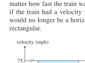
Applying the well-known formula distancerate time,we find that the answer is 150 miles. Simple. Now suppose that you are Isaac Newton trying to make a connection between this formula and the graph of the velocity function.

You might notice that the distance traveled by the train (150 miles) is exactly the area

of the rectangle whose base is the time interval 7, 9and whose height at each point is the value of the constant velocity function v75 ( Figure 5.1). This is no accident, either, since the distance traveled and the area in this case are both found by multiplying the rate (75) by the change in time (2).

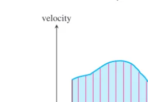
This same connection between distance traveled and rectangle area could be made no matter how fast the train was going or how long or short the time interval was. But what if the train had a velocity vthat varied as a function of time? The graph ( Figure 5.2) would no longer be a horizontal line, so the region under the graph would no longer be rectangular.

5.1

What you’ll learn about

• Distance Traveled

• Rectangular Approximation Method (RAM)

• Volume of a Sphere

• Cardiac Output

. . . and why

Learning about estimating with finite sums sets the foundation for understanding integral calculus.

velocity (mph)

75

7 9

0

[image:2.684.226.367.551.655.2]

time (h)

Figure 5.1 The distance traveled by a 75 mph train in 2 hours is 150 miles, which cor-responds to the area of the shaded rectangle.

velocity

a

[image:2.684.429.576.552.652.2]

O b time

Would the area of this irregular region still give the total distance traveled over the time interval? Newton and Leibniz (and, actually, many others who had considered this question) thought that it obviously would, and that is why they were interested in a cal-culus for finding areas under curves. They imagined the time interval being partitioned into many tiny subintervals, each one so small that the velocity over it would essentially be constant. Geometrically, this was equivalent to slicing the irregular region into nar-row strips, each of which would be nearly indistinguishable from a narnar-row rectangle ( Figure 5.3).

velocity

a b

O time

v

1

0 2 3

9

v = t2

t v

0.5 0.75

0 1 t

[image:3.684.310.454.149.249.2]

v t2

Figure 5.3 The region is partitioned into vertical strips. If the strips are narrow enough, they are almost indistinguishable from rectangles. The sum of the areas of these “rectangles” will give the total area and can be interpreted as distance traveled.

Figure 5.4 The region under the parabola v t2_{from t 0 to t 3 is partitioned into} 12 thin strips, each with base t 14. The strips have curved tops. ( Example 1)

Figure 5.5 The area of the shaded re-gion is approximated by the area of the rectangle whose height is the function value at the midpoint of the interval. ( Example 1)

They argued that, just as the total area could be found by summing the areas of the (essentially rectangular) strips, the total distance traveled could be found by summing the small distances traveled over the tiny time intervals.

EXAMPLE 1 Finding Distance Traveled when Velocity Varies

A particle starts at x 0 and moves along the x-axis with velocity vt t2 _{for time} t 0. Where is the particle at t 3?

SOLUTION

We graph vand partition the time interval 0, 3into subintervals of length Dt. (Figure 5.4 shows twelve subintervals of length 3

12 each.)

Notice that the region under the curve is partitioned into thin strips with bases of length 1

4 and curvedtops that slope upward from left to right. You might not know how to find the area of such a strip, but you can get a good approximation of it by finding the area of a suitable rectangle. In Figure 5.5, we use the rectangle whose height is the

y-coordinate of the function at the midpoint of its base.

Table 5.1

Subinterval

[

0 ,1

4

]

[

1 4,

1

2

]

[

1 2,

3

4

]

[

3 4, 1

]

Midpoint m_i 1

8 3

8 5

8 7 8 Height mi2 ₆

1 4

₆9₄ 2₆5₄ 4₆9₄ Area 1

4mi2

2 1

56 2 9

56 2 2 5

5 6

2 4

5 9

6

y

3 x

y

3 x

y

3 x

Figure 5.7 LRAM, MRAM, and RRAM approximations to the area under the graph of yx2_{from x0 to x3.}

v

1

0 2 3

9

t v t2

Figure 5.6 These rectangles have ap-proximately the same areas as the strips in Figure 5.4. Each rectangle has height m_i2_, where miis the midpoint of its base.

( Example 1)

The area of this narrow rectangle approximates the distance traveled over the time subinterval. Adding all the areas (distances) gives an approximation of the total area under the curve (total distance traveled) from t 0 to t 3 ( Figure 5.6). Computing this sum of areas is straightforward. Each rectangle has a base of length Dt 1

4, while the height of each rectangle can be found by evaluating the function at the midpoint of the subinterval. Table 5.1 shows the computations for the first four rectangles.

Approximation by Rectangles

Approximating irregularly-shaped re-gions by regularly-shaped rere-gions for the purpose of computing areas is not new. Archimedes used the idea more than 2200 years ago to find the area of a circle, demonstrating in the process that was located between 3.140845 and 3.142857. He also used approxima-tions to find the area under a parabolic arch, anticipating the answer to an im-portant seventeenth-century question nearly 2000 years before anyone thought to ask it. The fact that we still measure the area of anything—even a circle—in “square units” is obvious testimony to the historical effectiveness of using rectangles for approximating areas.

Continuing in this manner, we derive the area 1

4mi2 _{for each of the twelve}

subin-tervals and add them:

₂1_{56 2}9_{56 2}2₅ 5_{6 2}4₅9 _{6 2}8₅ 1₆ 1₂2₅ 1₆ 1₂₅6 9₆ 2₂2₅5₆

2 2 8 5 9 6

3

2 6 5 1 6

4

2 4 5 1 6

5

2 2 5 9 6

2

2 3

5 0

6 0

8.98.

Since this number approximates the area and hence the total distance traveled by the particle, we conclude that the particle has moved approximately 9 units in 3 seconds. If it starts at x 0, then it is very close to x 9 when t 3. Now try Exercise 3.

To make it easier to talk about approximations with rectangles, we now introduce some new terminology.

Rectangular Approximation Method (RAM)

In Example 1 we used the Midpoint Rectangular Approximation Method (MRAM) to approximate the area under the curve. The name suggests the choice we made when deter-mining the heights of the approximating rectangles: We evaluated the function at the mid-point of each subinterval. If instead we had evaluated the function at the left-hand endmid-point we would have obtained the LRAMapproximation, and if we had used the right-hand end-points we would have obtained the RRAM approximation. Figure 5.7 shows what the three approximations look like graphically when we approximate the area under the curve y x2

No matter which RAM approximation we compute, we are adding products of the form

fxi•x, or, in this case,xi2•3

6.

LRAM:

(

0

)

2

(

1₂

)

(

1₂

)

2

(

1₂

)

(

1

)

2

(

1₂

)

(

3₂

)

2

(

1₂

)

(

2

)

2

(

1₂

)

(

5₂

)

2

(

1₂

)

6.875 MRAM:

(

1 4

)

2

(

1

2

)

(

3 4

)

2

(

1

2

)

(

5 4

)

2

(

1

2

)

(

7 4

)

2

(

1

2

)

(

9 4

)

2

(

1

2

)

(

1 4

1

)

2

(

1

2

)

8.9375

RRAM:

(

1₂

)

2

(

1₂

)

(

1

)

2

(

1₂

)

(

3₂

)

2

(

1₂

)

(

2

)

2

(

1₂

)

(

5₂

)

2

(

1₂

)

(

3

)

2

(

1₂

)

11.375 As we can see from Figure 5.7, LRAM is smaller than the true area and RRAM is larger. MRAM appears to be the closest of the three approximations. However, observe what happens as the number nof subintervals increases:

We computed the numbers in this table using a graphing calculator and a summing pro-gram called RAM. A version of this propro-gram for most graphing calculators can be found in the Technology Resource Manual that accompanies this textbook. All three sums

approach the same number (in this case, 9).

EXAMPLE 2 Estimating Area Under the Graph of a Nonnegative Function

Figure 5.8 shows the graph of fx)x2_{sinx on the interval 0, 3. Estimate the area}

under the curve from x0 to x3.

SOLUTION

We apply our RAM program to get the numbers in this table.

It is not necessary to compute all three sums each time just to approximate the area, but we wanted to show again how all three sums approach the same number. With 1000 subin-tervals, all three agree in the first three digits. (The exactarea is 7 cos 36 sin 32, which is 5.77666752456 to twelve digits.) Now try Exercise 7.

n LRAMn MRAMn RRAMn

5 5.15480 5.89668 5.91685 10 5.52574 5.80685 5.90677 25 5.69079 5.78150 5.84320 50 5.73615 5.77788 5.81235 100 5.75701 5.77697 5.79511 1000 5.77476 5.77667 5.77857 n LRAMn MRAMn RRAMn

6 6.875 8.9375 11.375 12 7.90625 8.984375 10.15625 24 8.4453125 8.99609375 9.5703125 48 8.720703125 8.999023438 9.283203125 100 8.86545 8.999775 9.13545 1000 8.9865045 8.99999775 9.0135045

[0, 3] by [–1, 5]

Volume of a Sphere

Although the visual representation of RAM approximation focuses on area, remember that our original motivation for looking at sums of this type was to find distance traveled by an object moving with a nonconstant velocity. The connection between Examples 1 and 2 is that in each case, we have a functionfdefined on a closed interval and estimate what we want to know with a sum of function values multiplied by interval lengths. Many other physical quantities can be estimated this way.

EXAMPLE 3 Estimating the Volume of a Sphere

Estimate the volume of a solid sphere of radius 4.

SOLUTION

We picture the sphere as if its surface were generated by revolving the graph of the function

fx16x2 _{about the x-axis (Figure 5.9a). We partition the interval 4 x 4}

into nsubintervals of equal length x8

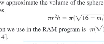
n. We then slice the sphere with planes perpen-dicular to the x-axis at the partition points, cutting it like a round loaf of bread into n paral-lel slices of width x. When nis large, each slice can be approximated by a cylinder, a familiar geometric shape of known volume,r2_{h. In our case, the cylinders lie on their}

sides and his xwhile rvaries according to where we are on the x-axis (Figure 5.9b). A logical radius to choose for each cylinder is fmi16mi2, where miis the midpoint

of the interval where the ith_{slice intersects the x-axis (Figure 5.9c).}

We can now approximate the volume of the sphere by using MRAM to sum the cylin-der volumes,

r2_h16m i22x.

The function we use in the RAM program is 16x22_16x2_{. The}

inter-val is 4, 4.

Number of Slices (n) MRAM_n 10 269.42299 25 268.29704 50 268.13619 100 268.09598 1000 268.08271 Which RAM is the Biggest?

You might think from the previous two RAM tables that LRAM is always a little low and RRAM a little high, with MRAM somewhere in between. That, however, depends on nand on the shape of the curve.

1. Graph y54 sinx

2 in the window 0, 3by 0, 5. Copy the graph on paper and sketch the rectangles for the LRAM, MRAM, and RRAM sums with

n3. Order the three approximations from greatest to smallest.

2. Graph y2 sin 5x3 in the same window. Copy the graph on paper and sketch the rectangles for the LRAM, MRAM, and RRAM sums with n3. Order the three approximations from greatest to smallest.

3. If a positive, continuous function is increasing on an interval, what can we say about the relative sizes of LRAM, MRAM, and RRAM? Explain.

4. If a positive, continuous function is decreasing on an interval, what can we say about the relative sizes of LRAM, MRAM, and RRAM? Explain.

EXPLORATION 1

y⎯⎯⎯⎯⎯⎯16 x2

x y

–4 0 4

(a)

√

x2

16

y =

x y

(b)

⎯⎯⎯⎯⎯⎯ √

x y

4 – 4

mi2

16 mi,

mi

x 16 2

y =

(c)

)

)

⎯⎯⎯⎯⎯⎯

[image:6.684.296.478.621.698.2]

√ √⎯⎯⎯⎯⎯⎯

Figure 5.9 (a) The semicircle y16x2_{revolved about the x-axis} to generate a sphere. (b) Slices of the solid sphere approximated with cylinders (drawn for n 8). (c) The typical approximating cylinder has radius

t c

0 2

5

Time (sec)

Dye concentration (mg/L)

4 6 8

7 9 11 15 19 23 27 31

[image:7.684.35.191.301.532.2]

cf(t)

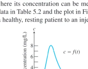
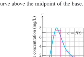
[image:7.684.303.452.364.480.2]

Figure 5.10 The dye concentration data from Table 5.2, plotted and fitted with a smooth curve. Time is measured with t 0 at the time of injection. The dye concentration is zero at the beginning while the dye passes through the lungs. It then rises to a maximum at about t 9 sec and tapers to zero by t 31 sec.

Table 5.2 Dye Concentration Data

Dye Seconds Concentration

after (adjusted for Injection recirculation)

t c

5 0 7 3.8 9 8.0 11 6.1 13 3.6 15 2.3 17 1.45 19 0.91 21 0.57 23 0.36 25 0.23 27 0.14 29 0.09 31 0

The value for n1000 compares veryfavorably with the true volume,

V 4

3r

3 4

34

3 25

3 6

268.0825731.

Even for n10 the difference between the MRAM approximation and the true vol-ume is a small percentage of V:

0.005.

That is, the error percentage is about one half of one percent! Now try Exercise 13.

Cardiac Output

So far we have seen applications of the RAM process to finding distance traveled and vol-ume. These applications hint at the usefulness of this technique. To suggest its versatility we will present an application from human physiology.

The number of liters of blood your heart pumps in a fixed time interval is called your

cardiac output. For a person at rest, the rate might be 5 or 6 liters per minute. During stren-uous exercise the rate might be as high as 30 liters per minute. It might also be altered sig-nificantly by disease. How can a physician measure a patient’s cardiac output without interrupting the flow of blood?

One technique is to inject a dye into a main vein near the heart. The dye is drawn into the right side of the heart and pumped through the lungs and out the left side of the heart into the aorta, where its concentration can be measured every few seconds as the blood flows past. The data in Table 5.2 and the plot in Figure 5.10 (obtained from the data) show the response of a healthy, resting patient to an injection of 5.6 mg of dye.

MRAM10256

3

256

3

MRAM10V

_V

Keeping Track of Units

Notice in Example 3 that we are sum-ming products of the form p16x2

(a cross section area, measured in square units) times Dx(a length, meas-ured in units). The products are there-fore measured in cubic units, which are the correct units for volume.

The graph shows dye concentration (measured in milligrams of dye per liter of blood) as a function of time (in seconds). How can we use this graph to obtain the cardiac output (measured in liters of blood per second)? The trick is to divide the number of mg of dyeby the area under the dye concentration curve.You can see why this works if you consider what happens to the units:

mg s

o e

f c

dye

•L

mg of

o b

f l

d o y o e d

L of se

b c

lood

.

So you are now ready to compute like a cardiologist. mg of dye

_Lmg_ofo_bf_ld_oy_oe_d •sec

mg of dye

EXAMPLE 4 Computing Cardiac Output from Dye Concentration

Estimate the cardiac output of the patient whose data appear in Table 5.2 and Figure 5.10. Give the estimate in liters per minute.

SOLUTION

[image:8.684.313.479.204.317.2]

We have seen that we can obtain the cardiac output by dividing the amount of dye (5.6 mg for our patient) by the area under the curve in Figure 5.10. Now we need to find the area. Our geometry formulas do not apply to this irregularly shaped region, and the RAM program is useless without a formula for the function. Nonetheless, we can draw the MRAM rectangles ourselves and estimate their heights from the graph. In Figure 5.11 each rectangle has a base 2 units long and a heightfmiequal to the height of the curve above the midpoint of the base.

Charles Richard Drew

(1904–1950)

Millions of people are alive today because of Charles Drew’s pioneering work on blood plasma and the preservation of human blood for transfusion. After directing the Red Cross program that collected plasma for the Armed Forces in World War II, Dr. Drew went on to become Head of Surgery at Howard University and Chief of Staff at Freedmen’s Hospital in Washington, D.C.

t c

0 2

5

Time (sec)

Dye concentration (mg/L)

4 6 8

7 9 11 15 19 23 27 31

cf(t)

Figure 5.11 The region under the concentration curve of Figure 5.10 is approximated with rec-tangles. We ignore the portion from t 29 to t 31; its concentration is negligible. ( Example 4) The area of each rectangle, then, is fmitimes 2, and the sum of the rectangular areas is the MRAM estimate for the area under the curve:

Areaf6•2f8•2f10•2…f28•2 2•1.46.37.54.82.81.91.1

0.70.50.30.20.1 2•27.655.2 mg

L•sec.

Dividing 5.6 mg by this figure gives an estimate for cardiac output in liters per second. Multiplying by 60 converts the estimate to liters per minute:

•6

1 0

m s i e

n c

6.09 L

min.

Now try Exercise 15.

5.6 mg _{55.2 mg}

•sec

L

Quick Review 5.1

As you answer the questions in Exercises 1–10, try to associate the answers with area, as in Figure 5.1.

1. A train travels at 80 mph for 5 hours. How far does it travel?

2. A truck travels at an average speed of 48 mph for 3 hours. How far does it travel? 144 miles

3. Beginning at a standstill, a car maintains a constant acceleration of 10 ftsec2_{for 10 seconds. What is its velocity after 10} seconds? Give your answer in ftsec and then convert it to mih.

4. In a vacuum, light travels at a speed of 300,000 kilometers per second. How many kilometers does it travel in a year? ( This distance equals one light-year.) 9.46 1012_km

5. A long distance runner ran a race in 5 hours, averaging 6 mph for the first 3 hours and 5 mph for the last 2 hours. How far did she run? 28 miles

6. A pump working at 20 gallonsminute pumps for an hour. How many gallons are pumped? 1200 gallons

400 miles

7. At 8:00 P.M. the temperature began dropping at a rate of 1 degree

Celsius per hour. Twelve hours later it began rising at a rate of 1.5 degrees per hour for six hours. What was the net change in temperature over the 18-hour period? 3°

8. Water flows over a spillway at a steady rate of 300 cubic feet per second. How many cubic feet of water pass over the spillway in one day? 25,920,000 ft3

9. A city has a population density of 350 people per square mile in an area of 50 square miles. What is the population of the city? 17,500 people

10.A hummingbird in flight beats its wings at a rate of 70 times per second. How many times does it beat its wings in an hour if it is in flight 70% of the time? 176,400 times

Section 5.1 Exercises

1. A particle starts at x0 and moves along the x-axis with velocity v(t) 5 for time t0. Where is the particle at t4?

2. A particle starts at x0 and moves along the x-axis with velocity v(t) 2t1 for time t 0. Where is the particle at t4?

3. A particle starts at x0 and moves along the x-axis with velocity v(t) t2 _{1 for time t 0. Where is the particle at} t4? Approximate the area under the curve using four rectangles of equal width and heights determined by the midpoints of the intervals, as in Example 1. See page 273.

4. A particle starts at x0 and moves along the x-axis with velocity v(t) t2 _{1 for time t 0. Where is the particle at} t5? Approximate the area under the curve using five rectangles of equal width and heights determined by the midpoints of the intervals, as in Example 1. See page 273. Exercises 5–8 refer to the region Renclosed between the graph of the function y2xx2 _{and the x-axis for 0 x 2.}

5. (a)Sketch the region R.

(b)Partition 0, 2into 4 subintervals and show the four rectangles that LRAM uses to approximate the area of R. Compute the LRAM sum without a calculator.

6. Repeat Exercise 1(b) for RRAM and MRAM.

7. Using a calculator program, find the RAM sums that complete the following table.

8. Make a conjecture about the area of the region R. The area is 4 3. In Exercises 9–12, use RAM to estimate the area of the region enclosed between the graph offand the x-axis for a x b.

9. fxx2_{x3, a0, b3 13.5}

10. fx 1

x, a1, b3 1.0986

11. fxex2_{, a0, b2 0.8821}

12. fxsinx, a0, b 2

13.(Continuation of Example 3) Use the slicing technique of Example 3 to find the MRAM sums that approximate the

n LRAMn MRAMn RRAMn

10 1.32 1.34 1.32

50 1.3328 1.3336 1.3328

100 1.3332 1.3334 1.3332

500 1.333328 1.333336 1.333328

volume of a sphere of radius 5. Use n 10, 20, 40, 80, and 160.

14.(Continuation of Exercise 13) Use a geometry formula to find the volumeVof the sphere in Exercise 13 and find (a)the error and (b)the percentage error in the MRAM approximation for each value of ngiven.

15. Cardiac Output The following table gives dye concentrations for a dye-concentration cardiac-output determination like the one in Example 4. The amount of dye injected in this patient was 5 mg instead of 5.6 mg. Use rectangles to estimate the area under the dye concentration curve and then go on to estimate the patient’s cardiac output. 44.8;6.7 L/min

t c

0 1

2

Time (sec)

Dye concentration (mg/L)

cf(t)

4 6 8 10 12 14 16 18 20 22 24 2

3 4

Seconds after Dye Concentration Injection (adjusted for recirculation)

t c

2 0 4 0.6 6 1.4 8 2.7 10 3.7 12 4.1 14 3.8 16 2.9 18 1.7 20 1.0 22 0.5 24 0 See page 273.

16.Distance Traveled The table below shows the velocity of a model train engine moving along a track for 10 sec. Estimate the distance traveled by the engine, using 10 subintervals of length 1 with (a)left-endpoint values (LRAM) and (b)right-endpoint values (RRAM). (a)87 in. 7.25 ft (b)87 in. 7.25 ft

17.Distance Traveled Upstream You are walking along the bank of a tidal river watching the incoming tide carry a bottle upstream. You record the velocity of the flow every 5 minutes for an hour, with the results shown in the table below. About how far upstream does the bottle travel during that hour? Find the (a)LRAM and (b)RRAM estimates using 12 subintervals of length 5. (a)5220 m (b)4920 m

18.Length of a Road You and a companion are driving along a twisty stretch of dirt road in a car whose speedometer works but whose odometer (mileage counter) is broken. To find out how long this particular stretch of road is, you record the car’s velocity at 10-sec intervals, with the results shown in the table below. ( The velocity was converted from mih to ftsec using 30 mih 44 ftsec.) Estimate the length of the road by averaging the LRAM and RRAM sums. 3665 ft

19.Distance from Velocity Data The table below gives data for the velocity of a vintage sports car accelerating from

0 to 142 mih in 36 sec (10 thousandths of an hour.) Time Velocity Time Velocity

sec ftsec sec ftsec

0 0 70 15 10 44 80 22 20 15 90 35 30 35 100 44 40 30 110 30 50 44 120 35 60 35

Time Velocity Time Velocity

min msec min msec

0 1 35 1.2 5 1.2 40 1.0 10 1.7 45 1.8 15 2.0 50 1.5 20 1.8 55 1.2 25 1.6 60 0 30 1.4

Time Velocity Time Velocity

sec in.sec sec in.sec

0 0 6 11 1 12 7 6 2 22 8 2 3 10 9 6 4 5 10 0 5 13

(a)Use rectangles to estimate how far the car traveled during the 36 sec it took to reach 142 mih. 0.969 mi

(b)Roughly how many seconds did it take the car to reach the halfway point? About how fast was the car going then?

20. Volume of a Solid Hemisphere To estimate the volume of a solid hemisphere of radius 4, imagine its axis of symmetry to be the interval 0, 4on the x-axis. Partition 0, 4into eight subintervals of equal length and approximate the solid with cylinders based on the circular

cross sections of the hemisphere perpendicular to the x-axis at the subintervals’ left endpoints. (See the accompanying profile view.)

(a)Writing to Learn Find the sum S8of the volumes of the cylinders. Do you expect S₈to overestimateV? Give reasons for your answer.

(b)Express VS8 as a percentage of Vto the nearest percent. 9%

Time (h)

Velocity (mph)

v

0 20

0.01 40

60 80 100 120 140 160

0.008 0.006 0.004

0.002 t Time Velocity Time Velocity

h mih h mih

0.0 0 0.006 116 0.001 40 0.007 125 0.002 62 0.008 132 0.003 82 0.009 137 0.004 96 0.010 142 0.005 108

x y

0

– 4

4 y⎯⎯⎯⎯⎯⎯⎯⎯16 x

2

4 3 2 1

√

0.006 h21.6 sec; 116 mph

S8146.08406

21. Repeat Exercise 20 using cylinders based on cross sections at the right endpoints of the subintervals. (a)S8120.95132

22.Volume of Water in a Reservoir A reservoir shaped like a hemispherical bowl of radius 8 m is filled with water to a depth of 4 m.

(a)Find an estimate Sof the water’s volume by approximating the water with eight circumscribed solid cylinders. 372.27873 m3

(b)It can be shown that the water’s volume is V3203 m3_. Find the error VS as a percentage of Vto the nearest percent. 11%

23.Volume of Water in a Swimming Pool A rectangular swimming pool is 30 ft wide and 50 ft long. The table below shows the depth hxof the water at 5-ft intervals from one end of the pool to the other. Estimate the volume of water in the pool using (a)left-endpoint values and (b)right-endpoint values.

24. Volume of a Nose Cone The nose “cone” of a rocket is a paraboloid obtained by revolving the curve yx, 0 x 5 about the x-axis, where xis measured in feet. Estimate the volume Vof the nose cone by partitioning 0, 5into five subintervals of equal length, slicing the cone with planes perpendicular to thex-axis at the subintervals’ left endpoints, constructing cylinders of height 1 based on cross sections at these points, and finding the volumes of these cylinders. (See the accompanying figure.) 31.41593

25.Volume of a Nose Cone Repeat Exercise 24 using cylinders based on cross sections at the midpoints of the subintervals.

26.Free Fall with Air Resistance An object is dropped straight down from a helicopter. The object falls faster and faster but its acceleration (rate of change of its velocity) decreases over time

x y

0 2

y√⎯x

3 4 5

1

Position ft Depth ft Position ft Depth ft x hx x hx

0 6.0 30 11.5 5 8.2 35 11.9 10 9.1 40 12.3 15 9.9 45 12.7 20 10.5 50 13.0 25 11.0

because of air resistance. The acceleration is measured in ftsec2_{and recorded every second after the drop for 5 sec, as} shown in the table below.

(a)Use LRAM₅to find an upper estimate for the speed when t5. 74.65 ft/sec

(b)Use RRAM5to find a lower estimate for the speed when t5. 45.28 ft/sec

(c)Use upper estimates for the speed during the first second, second second, and third second to find an upper estimate for the distance fallen when t3. 146.59 ft

27.Distance Traveled by a Projectile An object is shot straight upward from sea level with an initial velocity of 400 ft/sec.

(a)Assuming gravity is the only force acting on the object, give an upper estimate for its velocity after 5 sec have elapsed. Use g32 ftsec2_{for the gravitational constant. 240 ft/sec}

(b)Find a lower estimate for the height attained after 5 sec.

28. Water Pollution Oil is leaking out of a tanker damaged at sea. The damage to the tanker is worsening as evidenced by the increased leakage each hour, recorded in the table below.

(a)Give an upper and lower estimate of the total quantity of oil that has escaped after 5 hours. Upper: 758 gal; lower: 543 gal

(b)Repeat part (a) for the quantity of oil that has escaped after 8 hours. Upper: 2363 gal; lower: 1693 gal

(c)The tanker continues to leak 720 galh after the first 8 hours. If the tanker originally contained 25,000 gal of oil, approximately how many more hours will elapse in the worst case before all of the oil has leaked? in the best case?

29. Air Pollution A power plant generates electricity by burning oil. Pollutants produced by the burning process are removed by scrubbers in the smokestacks. Over time the scrubbers become less efficient and eventually must be replaced when the amount of pollutants released exceeds government standards.

Measurements taken at the end of each month determine the rate at which pollutants are released into the atmosphere as recorded in the table below.

Month Jan Feb Mar Apr May Jun Pollutant

Release Rate 0.20 0.25 0.27 0.34 0.45 0.52 (tonsday)

Month Jul Aug Sep Oct Nov Dec Pollutant

Release Rate 0.63 0.70 0.81 0.85 0.89 0.95 (tonsday)

Time (h) ⏐ 5 6 7 8 Leakage (galh)

⏐

265 369 516 720 Time (h) ⏐ 0 1 2 3 4 Leakage (galh)

⏐

50 70 97 136 190

t ⏐ 0 1 2 3 4 5

a

⏐

32.00 19.41 11.77 7.14 4.33 2.63 Underestimate (b)10%

(a)15,465 ft3 _{(b)16,515 ft}3

39.26991

1520 ft with RRAM and n5

(a)Assuming a 30-day month and that new scrubbers allow only 0.05 tonday released, give an upper estimate of the total tonnage of pollutants released by the end of June. What is a lower estimate? Upper: 60.9 tons; lower: 46.8 tons

(b)In the best case, approximately when will a total of 125 tons of pollutants have been released into the atmosphere?

30. Writing to Learn The graph shows the sales record for a company over a 10-year period. If sales are measured in millions of units per year, explain what information can be obtained from the area of the region, and why.

Standardized Test Questions

You should solve the following problems without using a graphing calculator.

31. True or False If fis a positive, continuous, increasing function on [a,b], then LRAM gives an area estimate that is less than the true area under the curve. Justify your answer.

32. True or False For a given number of rectangles, MRAM always gives a more accurate approximation to the true area under the curve than RRAM or LRAM. Justify your answer.

33. Multiple Choice If an MRAM sum with four rectangles of equal width is used to approximate the area enclosed between the x-axis and the graph of y4xx2_{, the approximation is E}

(A)10 (B)10.5 (C)10.6 (D)10.75 (E)11

34.Multiple Choice If fis a positive, continuous function on an interval [a,b], which of the following rectangular approximation methods has a limit equal to the actual area under the curve from ato bas the number of rectangles approaches infinity? D

III. LRAM

III. RRAM III. MRAM

(A)I and II only

(B)III only

(C)I and III only

(D)I, II, and III

(E)None of these

sales

10 0

20

time

35.Multiple Choice An LRAM sum with 4 equal subdivisions is used to approximate the area under the sine curve from x0 to xp. What is the approximation? C

(A)p

4

0

p 4 p 2 3 4 p

(B)p

4

0 1 2 2 3 1

(C)p

4

0 2 2 1 2 2

(D)p

4

0 1 2 2 2 2 3

(E)p

4

1 2 2 2 2 3 1

36.Multiple Choice A truck moves with positive velocity v(t) from time t3 to time t15. The area under the graph of yv(t) between 3 and 15 gives D

(A)the velocity of the truck at t15.

(B)the acceleration of the truck at t15.

(C)the position of the truck at t15.

(D)the distance traveled by the truck from t3 to t15.

(E)the average position of the truck in the interval from t3 to t15.

Exploration

37.Group Activity Area of a Circle Inscribe a regular n-sided polygon inside a circle of radius 1 and compute the area of the polygon for the following values of n.

(a)4 (square) (b)8 (octagon) (c)16

(d)Compare the areas in parts (a), (b), and (c) with the area of the circle.

Extending the Ideas

38.Rectangular Approximation Methods Prove or disprove the following statement: MRAMnis always the average of

LRAM_nand RRAM_n. False; look at f(x)x2_{, 0 x 1,n1.}

39.Rectangular Approximation Methods Show that iffis a nonnegative function on the interval a,band the line xab2 is a line of symmetry of the graph of yfx, then LRAM_nfRRAM_nffor every positive integer n.

40. (Continuation of Exercise 37)

(a)Inscribe a regular n-sided polygon inside a circle of radius 1 and compute the area of one of the ncongruent triangles formed by drawing radii to the vertices of the polygon.

(b)Compute the limit of the area of the inscribed polygon as n→∞.

(c)Repeat the computations in parts (a) and (b) for a circle of radius r.

1.Compute the area of the rectangle under the curve to find the particle is at x20.

2.Compute the area of the trapezoid under the curve to find the particle is at x20.

3.Each rectangle has base 1. The area under the curve is approximately

1

5 4

1 4

3

2₄9 5₄3

25, so the particle is close to x25.

4.Each rectangle has base 1. The area under the curve is approximately 1

5

4 1 4 3 2 4 9 5 4 3 8 4 5

46.25, so the particle is close to x46.25.

By the end of October

The area of the region is the total number of sales, in millions of units, over the 10-year period. The area units are (millions of units/year)years millions of units.

31.True. Because the graph rises from left to right, the left-hand rectangles will all lie under the curve.

32.False. For example, all three approximations are the same if the function is constant.

37. (a)2 (b)222.828 (c)8 sin

p 8

3.061

(d)Each area is less than the area of the circle,p. As nincreases, the polygon area approaches p.

39.RRAMnfLRAMnff(xn)Δx – f(x0)Δx

Definite Integrals

Riemann Sums

In the preceding section, we estimated distances, areas, and volumes with finite sums. The terms in the sums were obtained by multiplying selected function values by the lengths of intervals. In this section we move beyond finite sums to see what happens in the limit, as the terms become infinitely small and their number infinitely large.

Sigma notation enables us to express a large sum in compact form:

5.2

What you’ll learn about

• Riemann Sums

• Terminology and Notation of Integration

• The Definite Integral

• Computing Definite Integrals on a Calculator

• Integrability

. . . and why

The definite integral is the basis of integral calculus, just as the derivative is the basis of differential calculus.

The Greek capital letter

(sigma) stands for “sum.” The index ktells us where to begin the sum (at the number below the

) and where to end (at the number above). If the sym-bol

∞

appears above the

, it indicates that the terms go on indefinitely.

The sums in which we will be interested are calledRiemann (“ree-mahn”) sums,after Georg Friedrich Bernhard Riemann (1826–1866). LRAM, MRAM, and RRAM in the pre-vious section are all examples of Riemann sums—not because they estimated area, but because they were constructed in a particular way. We now describe that construction for-mally, in a more general context that does not confine us to nonnegative functions.

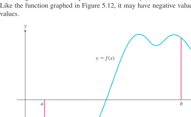
We begin with an arbitrary continuous functionfxdefined on a closed interval a,b. Like the function graphed in Figure 5.12, it may have negative values as well as positive values.

_k1n aka1a2a3…an1an.

We then partition the interval a,binto nsubintervals by choosing n1 points, say x1, x2, …,xn1, between aand bsubject only to the condition that

ax1x2…xn1b.

To make the notation consistent, we denote aby x0and bby xn. The set P{x0,x1,x2, …,xn}

is called a partition of a,b.

x y

b a

[image:13.684.228.538.388.578.2]

y f(x)

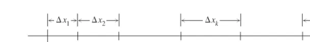
The partition Pdetermines nclosed subintervals, as shown in Figure 5.13. The kth

subinterval is xk1,xk, which has length xkxkxk1.

x

x_n

x_nb x_n1

x_k

x_k1 x_k

x₂

x ₂ x₁

x₁

[image:14.684.243.547.83.125.2]

x₀a _{• • • • • •}

Figure 5.13 The partition P{ax₀,x₁,x₂, …,x_nb} divides a,binto nsubintervals of lengths x1,x2, …,xn. The kthsubinterval has length xk.

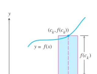
In each subinterval we select some number. Denote the number chosen from the kth

subinterval by ck.

Then, on each subinterval we stand a vertical rectangle that reaches from the x-axis to touch the curve at ck,fck. These rectangles could lie either above or below the x-axis ( Figure 5.14).

x y

y f(x)

0 x0 a x1 x2 xn b

c₁ c₂ c_k

(c₂, f(c₂)) (c₁, f(c₁))

c_n x_{n – 1} x_k

(c_n, f(c_n))

(c_k, f(c_k))

kth rectangle

[image:14.684.236.547.246.445.2]

x_{k – 1}

Figure 5.14 Rectangles extending from the x-axis to intersect the curve at the points ck, fck. The rectangles approximate the region between the x-axis and the

graph of the function.

On each subinterval, we form the product fck•xk. This product can be positive,

negative, or zero, depending onfck. Finally, we take the sum of these products:

Sn

n k1

fck•xk.

This sum, which depends on the partition P and the choice of the numbers ck, is a

Riemann sum forfon the interval [a,b].

As the partitions of a, b become finer and finer, we would expect the rectangles defined by the partitions to approximate the region between the x-axis and the graph off

with increasing accuracy ( Figure 5.15).

Just as LRAM, MRAM, and RRAM in our earlier examples converged to a common value in the limit,allRiemann sums for a given function on a,bconverge to a common value, as long as the lengths of the subintervals all tend to zero. This latter condition is assured by requiring the longest subinterval length (called the norm of the partition and denoted byP) to tend to zero.

(a) 0 a

y

x b yf(x)

(b) 0

yf(x)

a y

x b

Figure 5.15 The curve of Figure 5.12 with rectangles from finer partitions of

[image:14.684.54.199.408.643.2]

Despite the potential for variety in the sums

fckxkas the partitions change and as the ck’s are chosen arbitrarily in the intervals of each partition, the sums always have the same limit as P→0 as long asfis continuouson a,b.

THEOREM 1 The Existence of Definite Integrals

All continuous functions are integrable. That is, if a functionfis continuous on an in-terval a,b, then its definite integral over a,bexists.

The Definite Integral of a Continuous Function on [a, b]

Let f be continuous on a,b, and let a,b be partitioned into nsubintervals of equal length xba

n. Then the definite integral offover a,bis given by

lim

n→∞

n k1

fckx,

where each ckis chosen arbitrarily in the kth_subinterval.

Because of Theorem 1, we can get by with a simpler construction for definite integrals of continuous functions. Since we know for these functions that the Riemann sums tend to the same limit for allpartitions in which P→0, we need only to consider the limit of the so-called regular partitions, in which all the subintervals have the same length.

Terminology and Notation of Integration

Leibniz’s clever choice of notation for the derivative,dy

dx, had the advantage of retaining an identity as a “fraction” even though both numerator and denominator had tended to zero. Although not really fractions, derivatives can behavelike fractions, so the notation makes profound results like the Chain Rule

_ddy _{x d}d_uy •d d u x

seem almost simple.

Georg Riemann

(1826-1866) The mathematicians of the 17th and 18th centuries blithely as-sumed the existence of limits of Riemann sums (as we admittedly did in our RAM explorations of the last section), but the existence was not established mathematically until Georg Riemann proved Theorem 1 in 1854. You can find a current version of Riemann’s proof in most advanced calculus books.

DEFINITION The Definite Integral as a Limit of Riemann Sums

Letf be a function defined on a closed interval a,b. For any partition Pof a,b, let the numbers ckbe chosen arbitrarily in the subintervals xk1,xk.

If there exists a number Isuch that

lim

P→0

n k1

fckxkI

no matter how Pand the ck’s are chosen, then fis integrableon a,band Iis the

The notation that Leibniz introduced for the definite integral was equally inspired. In his derivative notation, the Greek letters (“” for “difference”) switch to Roman letters (“d” for “differential”) in the limit,

lim

x→0 y

x _ddy_x.

In his definite integral notation, the Greek letters again become Roman letters in the limit,

lim

n→∞

n k1

fckx

b

a

fxdx.

Notice that the difference Dxhas again tended to zero, becoming a differential dx. The Greek “

” has become an elongated Roman “S,” so that the integral can retain its identity as a “sum.” The ck’s have become so crowded together in the limit that we no longer think of

a choppy selection of xvalues between a and b, but rather of a continuous, unbroken sam-pling of xvalues from ato b. It is as if we were summing allproducts of the formfxdxas

xgoes from a to b, so we can abandon thekand the nused in the finite sum expression. The symbol

b a

fxdx

is read as “the integral from ato boffof xdee x,” or sometimes as “the integral from ato

bof fof xwith respect to x.” The component parts also have names:

b

a

f

x

dx

The value of the definite integral of a function over any particular interval depends on the function and not on the letter we choose to represent its independent variable. If we decide to use tor uinstead of x, we simply write the integral as

b a

ftdt or

b

a

fudu instead of

b

a

fxdx.

No matter how we represent the integral, it is the same number,defined as a limit of Riemann sums. Since it does not matter what letter we use to run from ato b, the variable of integra-tion is called a dummy variable.

EXAMPLE 1 Using the Notation

The interval 1, 3is partitioned into nsubintervals of equal length Dx4

n. Let mk

denote the midpoint of the kth_{subinterval. Express the limit}

lim

n_→∞

n

k1

3mk2_2mk5x

as an integral.

Upper limit of integration _{The function is theintegrand.}

xis thevariable of integration. Integral sign

Lower limit of integration

Integral of ffrom ato b

When you find the value of the integral, you have

evaluated the integral.

SOLUTION

Since the midpoints mkhave been chosen from the subintervals of the partition, this expression is indeed a limit of Riemann sums. (The points chosen did not have to be midpoints; they could have been chosen from the subintervals in any arbitrary fashion.) The function being integrated is fx3x2_{2x5 over the interval 1, 3.}

Therefore,

lim

n→∞

n

k1

3mk2_2mk5x

3

1

3x2_2x5dx.

Now try Exercise 5.

Definite Integral and Area

If an integrable function yfx is nonnegative throughout an interval a, b, each nonzero termfckxkis the area of a rectangle reaching from the x-axis up to the curve

yfx. (See Figure 5.16.) The Riemann sum

fckxk,

which is the sum of the areas of these rectangles, gives an estimate of the area of the region between the curve and the x-axis from ato b. Since the rectangles give an increasingly good approximation of the region as we use partitions with smaller and smaller norms, we call the limiting value the area under the curve.

This definition works both ways: We can use integrals to calculate areas andwe can use areas to calculate integrals.

EXAMPLE 2 Revisiting Area Under a Curve

Evaluate the integral

₂2 4x2_dx.

SOLUTION

We recognize fx4x2 _{as a function whose graph is a semicircle of radius 2}

centered at the origin (Figure 5.17.

The area between the semicircle and the x-axis from 2 to 2 can be computed using the geometry formula

Area 1 2•r

2 1

2•2

2_2.

Because the area is also the value of the integral off from 2 to 2,

2

2

4x2 _{dx2. Now try Exercise 15.}

y

x

0

x_k x_k c_k x_k–1

f(c_k) (c_k, f(c_k))

y = f(x)

[image:17.684.32.192.153.275.2]

[–3, 3] by [–1, 3]

Figure 5.16 A term of a Riemann sum

fc_kx_kfor a nonnegative functionf is either zero or the area of a rectangle such as the one shown.

Figure 5.17 A square viewing window on y 4x2_{. The graph is a} semicir-cle because y 4x2_{is the same as} y2 _{4 x}2_{, or x}2 _y2 _{4, with y 0.} ( Example 2)

DEFINITION Area Under a Curve (as a Definite Integral)

If yfxis nonnegative and integrable over a closed interval a,b, then the area under the curve yfxfromato bis the integral of ffrom ato b,

A

b

a

[image:17.684.43.190.498.611.2]

If an integrable function yfx is nonpositive, the nonzero terms fckxkin the Riemann sums forfover an interval a,bare negatives of rectangle areas. The limit of the sums, the integral of f from ato b, is therefore the negative of the area of the region between the graph offand the x-axis ( Figure 5.18).

b a

fxdx (the area) if fx 0.

Or, turning this around, y = cos x

2

y

x

0 1

[image:18.684.53.198.53.131.2]

3 2

Figure 5.18 Because fx cosxis nonpositive on 2, 32, the integral of fis a negative number. The area of the shaded region is the opposite of this integral,

Area

32

2

cosx dx.

Area

b

a

fxdx when fx 0.

b a

fxdx(area above the x-axis) (area below the x-axis).

If an integrable function yfxhas both positive and negative values on an interval

a,b, then the Riemann sums forfon a,badd areas of rectangles that lie above the x-axis to the negatives of areas of rectangles that lie below the x-axis, as in Figure 5.19. The result-ing cancellations mean that the limitresult-ing value is a number whose magnitude is less than the total area between the curve and the x-axis. The value of the integral is the area above the

x-axis minus the area below. For any integrable function,

Finding Integrals by Signed Areas

It is a fact (which we will revisit) that

₀sinx dx2 ( Figure 5.20). With that in-formation, what you know about integrals and areas, what you know about graph-ing curves, and sometimes a bit of intuition, determine the values of the followgraph-ing integrals. Give as convincing an argument as you can for each value, based on the graph of the function.

1.

2

sinx dx 2.

2

0

sinx dx 3.

2

0

sinx dx

4.

0

2sinxdx 5.

0

2 sinx dx 6.

2

2

sinx2dx

7.

sinu du 8.

2

0

sinx

2dx 9.

0

cosx dx

10.Suppose kis anypositive number. Make a conjecture about

k_ksinx dx and support your conjecture.

EXPLORATION 1

x y

0

yf(x)

If f(c_k) 0, f(c_k)x_k is an area…

…but if f(c_k) 0, f(c_k)x_k is the negative of an area.

a b

Net Area

Sometimes _abfxdxis called the

net areaof the region determined by the curve y fxand the

[image:18.684.42.204.190.375.2]

x-axis between x aand x b. Figure 5.19 An integrable functionf with negative as well as positive values.

[– , ] by [–1.5, 1.5]

y sin x

Figure 5.20

0

[image:18.684.229.514.525.636.2]

Constant Functions

[image:19.684.316.490.244.355.2]

Integrals of constant functions are easy to evaluate. Over a closed interval, they are sim-ply the constant times the length of the interval ( Figure 5.21).

Figure 5.21 (a) If cis a positive con-stant, then _abc dx is the area of the rectan-gle shown. (b) If cis negative, then _abc dx is the opposite of the area of the rectangle. x

y y

x c

c

(a, c)

(a, c) (b, c) (b, c)

a

a b

b

(a)

(b)

A = c(b–a) = b

ac dx ⌠ ⌡

⌠ ⌡

A= (– c)(b–a) = – b

ac dx

THEOREM 2 The Integral of a Constant

If fxc, where cis a constant, on the interval a,b, then

b a

fxdx

b

a

c dxcba.

Proof A constant function is continuous, so the integral exists, and we can evaluate it as a limit of Riemann sums with subintervals of equal length ba

n. Any such sum looks like

_k1n fck•x, which is

n

k1 c•b

n a

.

Then

n

k1 c•b

n a

c•ba

n

k1 1

n

cba•n

(

1 n

)

cba.

Since the sum is always cbafor any value of n,it follows that the limit of the sums, the integral to which they converge, is also cba. ■

EXAMPLE 3 Revisiting the Train Problem

A train moves along a track at a steady 75 miles per hour from 7:00 A.M. to 9:00 A.M. Express its total distance traveled as an integral. Evaluate the integral using Theorem 2.

SOLUTION (See Figure 5.22.)

velocity (mph)

75

7 9

time (h)

Distance traveled

9

7

75dt75•97150

Since the 75 is measured in miles

hour and the 97is measured in hours, the 150 is measured in miles. The train traveled 150 miles. Now try Exercise 29.

Integrals on a Calculator

You do not have to know much about your calculator to realize that finding the limit of a Riemann sum is exactly the kind of thing that it does best. We have seen how effectively it can approximate areas using MRAM, but most modern calculators have sophisticated built-in programs that converge to built-integrals with much greater speed and precision than that. We will assume that your calculator has such a numerical integration capability, which we will denote as NINT.In particular, we will use NINT fx,x,a,bto denote a calculator (or computer) approximation of

_abfxdx. When we write

b a

fxdxNINTfx,x,a,b,

we do so with the understanding that the right-hand side of the equation is an approxima-tion of the left-hand side.

EXAMPLE 4 Using NINT

Evaluate the following integrals numerically.

(a)

2 1

xsinx dx (b)

1

0

₁4_x2 dx (c)

5

0

ex2

dx

SOLUTION

(a)NINTxsin x,x,1, 2 2.04

(b)NINT 4

1x2_{,x, 0, 1 3.14} (c)NINTex2

,x, 0, 5 0.89 Now try Exercise 33.

We will eventually be able to confirm that the exact value for the integral in Example 4a is 2 cos 2 sin 2 cos 1 sin 1. You might want to conjecture for yourself what the exact answer to Example 4b might be. As for Example 4c, no explicit exact value has ever been found for this integral! The best we can do in this case (and in many like it) is to approximate the integral numerically. Here, technology is not only useful, it is essential.

Discontinuous Integrable Functions

Theorem 1 guarantees that all continuous functions are integrable. But some functions with discontinuities are also integrable. For example, a bounded function (see margin note) that has a finite number of points of discontinuity on an interval a,bwill still be integrable on the interval if it is continuous everywhere else.

EXAMPLE 5 Integrating a Discontinuous Function

Find

2 1

dx.

SOLUTION

This function has a discontinuity at x 0, where the graph jumps from y 1 to

y 1. The graph, however, determines two rectangles, one below the x-axis and one above ( Figure 5.23).

Using the idea of net area, we have

2 1

dx 1 2 1. Now try Exercise 37.

x

x x

x

Bounded Functions

We say a function is boundedon a given domain if its range is confined be-tween some minimum value mand some maximum value M. That is, given any xin the domain, m fx M. Equivalently, the graph of yfxlies between the horizontal lines ymand

yM.

y = |x|/x

[image:20.684.221.497.241.370.2]

[–1, 2] by [–2, 2]

Figure 5.23 A discontinuous integrable function:

2

1

In Exercises 1–3, evaluate the sum.

1.

5

n1

n2 _{55 2.}

4

k0

3k2 20

3.

4

j0

100j12 ₅₅₀₀

In Exercises 4–6, write the sum in sigma notation.

4. 123…9899

5. 024…4850

6. 312₃₂2…₃₅₀₀2

More Discontinuous Integrands

1. Explain why the function

fx x x

2

2 4

is not continuous on 0, 3. What kind of discontinuity occurs?

2. Use areas to show that

3 0 x x 2 2 4

dx10.5.

3. Use areas to show that

5 0

intxdx10.

EXPLORATION 2

A Nonintegrable Function

How “bad” does a function have to be before it is notintegrable? One way to defeat integrability is to be unbounded (like y 1xnear x 0), which can pre-vent the Riemann sums from tending to a finite limit. Another, more subtle, way is to be bounded but badly discontinu-ous, like the characteristic function of the rationals:

1 if xis rational

fx

{

0 if xis irrational. No matter what partition we take of the closed interval 0, 1, every subinterval contains both rational and irrational numbers. That means that we can always form a Riemann sum with all rational ck’s (a Riemann sum of 1) or all

irrational ck’s (a Riemann sum of 0).

The sums can therefore never tend toward a unique limit.

Quick Review 5.2

In Exercises 7 and 8, write the expression as a single sum in sigma notation.

7. 2

50

x1

x2₃

50

x1

x 8.

8

k0

xk

20

k9 xk

20 k0 xk 9. Find

n k0

1k _{if nis odd.}

n

k0

(1)k_{0 if nis odd.}

10.Find

n k0

1k _{if nis even.}

n

k0

(1)k_{1 if nis even.}

Section 5.2 Exercises

In Exercises 1–6, each c_k is chosen from thekth subinterval of a regular partition of the indicated interval into nsubintervals of length

x. Express the limit as a definite integral.

1. lim

n→∞

n k1

c_k2_{x, 0, 2}

2

0

x2_dx

2. lim

n→∞

n k1

ck23ckx, 7, 5

5

7

(x2_{3x) dx}

3. lim

n→∞

n k1

c 1

k

x, 1, 4

4

1

1

xdx

4. lim

n→∞

n k1

1

1 c_k

x, 2, 3

3

2 1

1 x dx 5. lim n→∞

n k1

4c_k2_{x, 0, 1}

1

0

4x2_dx

6. lim

n→∞

n k1

sin3_c

kx, ,

p

p

sin3_{x dx}

In Exercises 7–12, evaluate the integral.

7.

1

2

5dx 15 8.

7

3

20dx 80

9.

3

0

160dt 480 10.

1

4

2du 3 2 p 11.

3.4 2.1

0.5ds 2.75 12.

2

18

2dr 4

99 k1 k

25 k0 2k

500 k1

3k2

50 x1