of peer-reviewed research and commentary in the population sciences published by the Max Planck Institute for Demographic Research Konrad-Zuse Str. 1, D-18057 Rostock · GERMANY www.demographic-research.org
DEMOGRAPHIC RESEARCH
VOLUME 12, ARTICLE 9, PAGES 197-236
PUBLISHED 04 MAY 2005
www.demographic-research.org/Volumes/Vol12/9
DOI: 10.4054/DemRes.2005.12.9
Research Article
World Urbanization Prospects:
an alternative to the UN model
of projection compatible with the
mobility transition theory
Philippe Bocquier
1 Introduction 198
2 An evaluation of the UN projections 200 2.1 Evidence of non-linearity in the relation between
urban-rural growth difference and the percentage urban
203
2.2 Evidence of overestimation in the projection of the proportion urban
207
3 In search or an alternative model for projecting urbanisation
207
3.1 Principle characteristics expected from a projection model for urbanisation
209
3.2 The underlying mathematics of the urban transition process
210
3.3 Model implementation 211
3.4 Corrections imposed on outliers 213
4 A comparison of the results obtained through the UN and the polynomial models of projection
216
5 Conclusions: improving projection models 223
6 Acknowledgements 226
References 227
Appendix I 230
World Urbanization Prospects:
an alternative to the UN model of projection compatible with the
mobility transition theory
Philippe Bocquier1
Abstract
This paper proposes to critically examine the United Nations projections on urbanisation. Both the estimates of current trends based on national data and the method of projec-tion are evaluated. The theory of mobility transiprojec-tion is used as an alternative hypothesis. Projections are proposed using a polynomial model and compared to the UN projections, which are based on a linear model. The conclusion is that UN projections may overesti-mate the urban population for the year 2030 by almost one billion, or 19% in relative term. The overestimation would be particularly more pronounced for developing countries and may exceed 30% in Africa, India and Oceania.
1. Introduction
The United Nations Population Division has been publishing and revising its World Ur-banisation Prospects since 1991 (the latest being the 2002 revision: United Nations 2002) and this has become a popular source of data and analysis of the past, current and fu-ture proportion urban in each country, region or continent of the world. As urban issues get more attention, notably in the Millennium Development Goals (MDG), it is increas-ingly used as an instrument for projections of some other global trends, such as poverty (UN-Habitat 2003; World Bank 2003), energy consumption (EIA 2004; IEA 2004), en-vironment and resources (UNDP et al. 2003), etc. Projections and even estimations, for recent years, of other global trends cannot afford to do without urbanisation projections, as they are often a key indicator of global integration. No other organisation than the UN has been successful in compiling a database on urbanisation that equals the UN database in scope and quality. An early attempt to offer alternative to the UN database is the GEOPOLIS database, which is using a common agglomeration (building-blocks density) and population (10,000 inhabitants threshold) criteria for all countries (Moriconi-Ebrard 1993, 1994). Unfortunately, this database is at present only available up to 1990 and its procedures have not been recognized by an international body. A more recent alterna-tive using polygons created from satellite images of night-time lights is offered by the Gridded Population of the World (GPW) database under construction at the Columbia University’s Earth Institute’s Center for International Earth Science Information Network (CIESIN) and available online (Balk et al. 2004). This last approach is promising but the data on urban agglomerations are not yet available world-wide and may reflect more the availability of electricity than the actual population size and density.
about the quality of the national urbanisation estimates and the method of projection used by the UN.
What about using national estimates rather than internationally-agreed estimates? The UN argues (1997, p160) that though “the quality of the estimates and projections made is highly dependent on the quality of the basic information permitting the calculation of the proportion urban” and that “the criteria used to identify urban areas vary from coun-try to councoun-try and may not be consistent even between different data sources within the same country”, it still relies “on the data produced by national sources that reflect the definitions and criteria established by national authorities”. This justification is based on UN reports published in the 1960s that concluded that “it is not possible or desirable to adopt uniform criteria to distinguish urban areas from rural areas”. This opinion will appear outdated to the 21st century reader: first, many attempts have been made since the 1960s to harmonise databases on urbanisation, at least at a regional level (European Union, CELADE), precisely to allow comparison across time and space. Maintaining the same definitions of urban areas might also enable time comparison for each particular country. Considering that most urban definitions are inadequate for analysis, the effort is now directed towards more flexible definitions using the building-block areas as the smallest units of analysis, thus permitting presentation along different criteria depending on the focus of the analysis (Hugo and Champion 2003). Therefore, the only remain-ing justification for usremain-ing national definitions is that the data based on those definitions are readily available, whereas more sophisticated definitions are still to be tested and ap-proved by national and international entities. That is the main reason why, despite its inadequacy and all scientific efforts to remedy it, the UN database will still be used for many years, unless considerable international effort is directed towards collecting data in a format that would be suitable for applying more flexible definition of urban areas. This reason only would suffice to develop a methodology to obtain proper projections using the currently available UN data based on national definitions.
for the estimation period 1950-1995. Though this is not clearly stated in the report, a number of LDC did not actually offer data on urbanisation for the 1990s and even for the 1980s and projections had to be made for these two decades. As our analysis will show, the projection method has an effect on the estimates of the urban population as early as in 1990.
Why should the projections be systematically biased? Why are LDC more affected by this bias than more developed countries (MDC)? The first part of this paper will demon-strate that these problems originate mainly in the regression model used in the method of projection. Are there alternative theories that could help to better hypothesize on urban-isation trends? The second part of this paper will present a refinement to the theory of mobility transition and will test its implications on urbanisation projections. An original method of projection will be considered and its results will be compared to the UN pro-jections. In this paper, to facilitate comparative reading, we adopt the same vocabulary and notations as found in the UN reports.
2. An evaluation of the UN projections
The principle of the UN interpolation (starting from 1st July 1950 to the end of the es-timation period, 1st July 1995) and extrapolation (same principle applies from 1995 to 2030) is based on the linear projection of the relevant inter-census urban-rural growth dif-ference, denotedrurin the UN reports. At any timet+1therurcan be noted, with rates
expressed in terms of the population at timetandt+1:
rur t+1 =u t+1 r t+1 = U t+1 U t U t R t+1 R t R t whereu t+1and r
t+1stands respectively for the urban and the rural growth rate in the
interval (t;t+1),U
tfor the urban population and R
tfor the rural population at time t. In
the general case, for any interval (t;t+n), theruris computed using the formula:
rur t+n = ln(U t+n =U t ) n ln(R t+n =R t ) n
The proportion urban (PU) at timeT within an intercensal period for interpolation,t < T <t+n, is determined by the equation:
PU T
=UR R T
=[1+UR R T
]
where
UR R T
=UR R t
exp[rur t+n
and
UR R t =U t =R t :
The same formula applies for extrapolation outside an intercensal period,t+n < T,
and theruris determined from the urban and rural populations of the closest intercensal
period (t;t+n) available (United Nations 2002).
To implement the UN projection model, one needs to know only the total population and the urban population (or the proportion urban) at different dates. All other quanti-ties are derived from these. The UN projection model belongs therefore to the class of endogenous autoregressive projection models. It is not explanatory as no independent, exogenous variables are introduced in the estimation.
It can be shown that the projection method described above mathematically overes-timates urban growth. As correctly stated in the UN report, the urban-rural growth dif-ference “declines as the proportion urban increases because the pool of potential rural-urban migrants decreases as a fraction of the rural-urban population, while it increases as a fraction of the rural population” (United Nations 2002, p106). Therefore, the UN has developed a model for the evolution of the hypothetical urban-rural growth difference (denotedhrurin the UN report). This model is “obtained by regressing the initial
ob-served percentage urban on the urban-rural differential for the 113 countries with more than 2 million inhabitants in 1995. [:::] The projection of the proportion urban is carried
out, based on a weighted average of the observed urban-rural growth difference for the most recent period available in a given country and the hypothetical urban-rural growth difference” (United Nations 2002, p111).
In practical terms, interpolations at specific dates from 1955 to 1995 (estimation pe-riod) are derived from therurcomputed using the intercensal data, as explained above,
whereas the UN model for urban projections is a weighted average of the preceding es-timation ofrur and of the hypothetical urban-rural growth difference for the projection
period (hrur) computed from a regression model ofruragainstPUas per 1995 in
coun-triesiof 2 millions inhabitants and more:
rur i;t+5 = W 1;t rur i;t +W 2;t hrur = W 1;t rur i;t +W 2;t
(0:037623 0:02604PU i;t
)
where
W 1;t
=0:8 W 2;t
=0:2 whent=1995 W
1;t
=0:6 W 2;t
=0:4 whent=2000 W
1;t
=0:4 W 2;t
=0:6 whent=2005 W
1;t
=0:2 W 2;t
=0:8 whent=2010 W
1;t
=0 W
2;t
The projection is conducted step by step, by five-year increment, the estimate for one projection period being used for the projection of the next.
The implications of such a method are the following:
Because the linear regression model is based on data compiled when the world
ur-ban transition was well on its way (the proportion urur-ban was 45.1% in 1995, with regions’ estimates ranging from a minimum of 21.9% in Eastern Africa to a max-imum of 87.4% in Australia/New-Zealand), it does not take into account the true relation between urban-rural growth difference and the percentage urban at the be-ginning and at the end of the urban transition from low to high proportion urban. As noted by an earlier critique (National Research Council 2003, p496), the declin-ing function has not only the effect of slowdeclin-ing down the urban growth of highly urbanised countries but it has also the effect of speeding the urbanisation process of little urbanised countries. According to the empirical equation mentioned above, one could theoretically have in some countries a 3.76%rur at the beginning of
the process when initial percentage urban is zero, though we expect from historical observation of countries with low percentage urban that therur be growing
pro-gressively from zero value. This is not however the main problem: historically, the
rur reached higher level than 4% or even 5% in some countries or regions (e.g.
in Melanesia when therurwas around 6% for an initial 11.5% percentage urban
in the late 1960s). The flaw is more at the other end of the process. We certainly cannot expect therurto reach 1.16% when the initial population is already 100%
urban, because when all the population is urban therur can only be zero or
neg-ative, leading to a decrease in the percentage urban. Very few countries of more than 2 million inhabitants (the threshold chosen to compute the regression model) can reach 100% urbanisation so the contradiction is not very likely to arise, but it is still important to incorporate in the model the trends at the limit. Therefore, with-out even considering the empirical data, a non-linear model would be more con-sistent with the mathematical relation between therur and the percentage urban.
In addition, considering the empirical data, the model should make provision for the quasi-stabilisation of urbanisation below 100%, as already observed in some, mostly developed countries.
Because the model is uniquely applied on all countries, it cannot take account of the
historical differences in the urban transition from one country to another. Applied to projections, the model makes the implicit assumption that all countries should go through the same process of urbanisation as the currently developed countries. Not only does this assumption appear Western-centred, but as we will see (it is best illustrated graphically) it does not even fit the current trends of therur for
countries according to their historical path in the urbanisation process. Therurhas
never been much higher than 3% in developed countries whereas it could reach 5% or more in developing countries. In other words, significant urban growth started in the 18th Century in developed countries in order to reach a 55% proportion urban in 1950 and have more rapidly progressed in the second half of the 20th century to reach 75% in 1995. The urbanisation in developing countries, on the contrary, starting from less than 10% in 1900, rapidly reached 18% in 1950 and 38% in 1995.
2.1 Evidence of non-linearity in the relation between urban-rural growth difference and the percentage urban
Ideally, we would want to draw historical trends of urbanisation for all countries of the world since the beginning of ages. No currently available database can offer such long trends, even for the more developed countries or for the last two centuries only. Actually, the earliest date at which one can have a reasonable picture of the urbanisation worldwide is 1950. Estimates for earlier periods exist but only for Europe (Bairoch 1985; Chandler 1987; de Vries 1984) and China (Chandler 1987; Liang 2001) (for a synthesis on both, see Woods 2003). It is therefore not easy to demonstrate what should be the form of the relation between urban-rural growth difference and the percentage urban during the early stage of the urbanisation process, especially outside Europe.
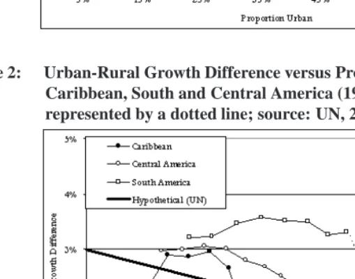
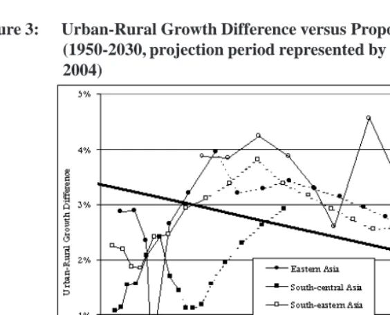
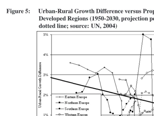
In figures 1 to 5, we plotted the trends formed by the urban-rural growth difference,
rur, in the (t 5;t) time interval against the proportion urban,PU, at timetfor different
regions of the world. The curves read from left to right and the first point represents the year 1955. Subsequent points are defined over five-year intervals until the year 2030, the last point on the curve. The projection period is represented for each region by dotted lines from 1990.
The reason why a linear model was used when the UN started its projection exercise in the 1980s was that at the time, very few countries had more than three observed points on therur-PUcurve from the 1950s to the 1970s. In absence of deeper historical trends,
a sensible solution was to model the trend across countries at a given time. The different level of urbanisation at which these countries were captured was supposed to reflect the most likely path the less urbanised countries would follow to reach, one day, the level of the most urbanised countries.
Now that data are available from the 1950s to the 1980s, and sometimes to the 1990s, there is less reason to believe that a linear model relatingrur andPU should still be
develop-Figure 1: Urban-Rural Growth Difference versus Proportion Urban in Africa (1950-2030, projection period represented by a dotted line; source: UN, 2004)
Figure 2: Urban-Rural Growth Difference versus Proportion Urban in
Figure 3: Urban-Rural Growth Difference versus Proportion Urban in Asia (1950-2030, projection period represented by a dotted line; source: UN, 2004)
Figure 5: Urban-Rural Growth Difference versus Proportion Urban in Developed Regions (1950-2030, projection period represented by a dotted line; source: UN, 2004)
ing countries (Eastern Africa, Middle Africa, Northern Africa, Caribbean, South-Central Asia, Melanesia and Micronesia) or in developed countries (Southern Europe and North-ern Europe). Other regions follow a more ambiguous pattNorth-ern but almost all have seen the
rurfalling sharply from peak values usually attained in the 1950s and 1960s for the LDC
regions, or in the 1970s and 1980s for the MDC regions. Exception to that phenomenon are found in Asia: Western Asia, which after a sharp fall in the 1970s, experienced the op-posite trend in the 1980s; South-Eastern Asia experienced a rise in the 1970s and 1980s, and Eastern Asia in the 1980s, though this can be attributed to China1only.
Rather intriguingly, some regions, particularly in Africa but also in Oceania, show a slight increase in therurin the 1980s that could be interpreted as a reversal of the overall
downward trend. However, this upward trend is limited and rather reflects the use of the UN model of projection for some countries where data were incomplete prior to 1995. This shows that the method not only has an effect on the 1995-2030 projection period but also on the later part of the estimation period, i.e. in the 1980s up to 1995, as data on urbanisation were not readily available for all developing countries.
1The peculiar case of China can be explained by the Cultural Revolution, which forced from the mid-1960s
2.2 Evidence of overestimation in the projection of the proportion urban
We have seen the urbanisation trends in the second half of the 20th century. Do the UN projections observe the same trends or do they depart significantly from the empirical, historical observations? The easiest way to confirm the latter is to observe the trends formed by the dotted lines on Figures 1 to 5 for the period 1990-2030. For ease of inter-pretation and in order to better show the effect of the UN model of projection, we added the regression result that was used to fit and to project the value ofrur.
Although the graphs show data grouped by world regions, whereas the UN estimation and projections were done country by country, it is clear that this method of projection has the effect of:
Reversing the downward trend for those regions which fell below the regression line
in 1995. This is particularly visible for developing Oceania and European regions (Figure 4 and 5), but also for other regions like Middle Africa (Figure 1) or South-Central Asia (Figure 3). In these regions, therur sort of ’bounced’ to reach the
level of the regression line.
For those regions which fell above the regression line in 1995, maintaining therur
at high level for some time before it joins the regression line.
Some other regions (South-Eastern Asia, Southern Africa, Central America and Australia-New Zealand) follow patterns that do not fit the above description, but generally, none of the trends for the projection period 1995-2030 follow the patterns of the estimation period 1950-1995, with the possible exceptions of Western Africa and Central America. The Figures make it clear that the UN projections are not prolonging historical trends. As expected – since the UN projection model applies uniformly to all countries –, all regions line up against the regression line in the vicinity of 2030.
What are the effects on the projected urbanisation level? The reversal of the down-ward trend and inflation of therur have the effect of increasing urban growth mostly in
developing countries, and maintaining urban growth at high level in developed countries. We then expect the projected proportion urban at the 2030 horizon to be largely overes-timated. In other words, the UN method of projection is implicitly imposing a unique, historically dated, MDC-oriented model of urban transition on all countries of the world, leading to a systematic overestimation of the world urbanisation.
3. In search for an alternative model for projecting urbanisation
develop-ment, measured either by gross domestic product (GDP) or by the human development index (HDI) (Davis and Henderson 2003; Njoh 2003; Woods 2003). Though the causal relationship between urbanisation and development is far from clear, an endogenous pro-jection model should apply differently depending on the specific urban history of the country at stake and should not necessarily lead to a high proportion urban for all coun-tries or regions of the world.
The theory of mobility transition initiated by W. Zelinsky (1971; 1983) offers an ideal type of a country which, starting from a low proportion urban and low urban growth, should go through a development process that leads to high urban growth. At the begin-ning of the mobility transition, urban growth is generally migration-driven whereas at its end the contribution of natural growth to the urban to rural growth differential is higher. At the end of the mobility transition, the country should reach a high proportion urban and low urban growth, as observed in the developed countries. Graphically, it means that the plot of theruragainst thePU should form an inverted U-curve, starting at 0% or so
and finishing maybe at 100%. The mobility transition theory recognised that each country might follow the urban transition at its own pace. This seems to be indeed the case, as some western countries took more than two centuries to reach their current level of ur-banisation whereas some other countries experienced the same transition in less than 50 years.
However this theory, is not clear about the effect of the development process on the actual level of urbanisation that each country should reach at the end of the mobility transition. It is hypothesized that development as it is known in the Western world should expand to the rest of the world so that, at the end of the day, all countries should reach the same level of urbanisation, close to the level reached in the present MDC. On the contrary, the empirical evidence of the preceding section shows that the urban transition might follow different patterns according to the historical period it went through and to the level of economic development reached. In statistical terms, the curve formed by plotting
ruragainstPU has different shapes. Not only the modal point of the curve varies a lot
(reaching a maximum of 6% in Melanesia, for example), but also the proportion urban at which therurseems to converge to zero is different.
We will call this point of convergence the urban saturation point for convenience. It represents the point where rural and urban areas are growing at the same pace. The term saturation as employed here does not mean it is an absorbing state where the country or region is trapped afterrur eventually reaches zero. In the real world of urbanisation,
cases of counterurbanisation (whenrur is less than 0) and erratic variations around a
focal point (whenruris alternatively greater and smaller than0) are not uncommon. Our
over time.
In this section, we will start by giving the principal characteristics of a model for urban projection before proposing a new model of projection based on two key principles: his-torical perspective and country-based approach. We will then implement the model and show that it actually fits well the observed urbanisation process of most countries in the world and offers a quite reasonable alternative to the UN projections, even with imperfect data. Note that our empirical model of urban transition does not pretend to exhaust the complexity of Zelinsky’s theoretical model of mobility transition, which is more compre-hensive in its attempt to integrate the demographic transition theory. However, the model of urban transition can help testing the validity of some of the hypotheses of the model of mobility transition regarding the evolution of urbanisation.
3.1 Principle characteristics expected from a projection model for urbanisation
To follow a historical perspective on urban transition, an alternative model of projection based on macro-data should integrate two new factors: speed of urban transition and possible urban saturation, or even counterurbanisation as seen in some developed coun-tries as early as in the 1970s (Champion 1989; 2000). The new models for projection should rely more on the past, empirically observed trends, and should keep the arbitrary choice to a minimum. The new projection model should be endogenous, i.e. based on the available data only, as the UN projection model is. Our objective here is not to offer a projection model with explanatory power, using a number of exogenous variables (such as GDP, HDI, etc.) that could explain the proportion urban and its trend, but to offer better projections using the known quantities only.
The model should take into account that projections do not necessarily converge to-ward an average behaviour. The model should allow each country or region to follow its own urban transition, leading to different level of urban saturation. A polynomial of second degree should ideally conform to the inverted-U shape historically observed up to 1995 in most countries and the projectedrur
will take the form:
rur i;t+5
=F(PU i;t
)= i;0
+ i;1
PU i;t
+ i;2
PU 2 i;t
:
As for the UN model, the projection will be conducted step by step, by five-year incre-ment, the estimate for one projection period being used for the projection of the next. Before going into the details of the implementation of the polynomial model, we will ex-plain why the excess total absolute increase in urban areas should be preferred to therur
3.2 The underlying mathematics of the urban transition process
The reader would have already noticed that the relation between the urban-rural growth difference (rur) and the proportion urban (PU) plays an important role in the UN
projec-tions. As noted in the UN report, theruris a difference of rates. As such, it does not take
account of the constraints imposed by the risk pool (the absolute number) in both urban and rural areas. Using intercensal rates seems perfectly sensible for interpolation because the census data represent observed boundaries and therefore the interpolation necessarily lies within the possible. For extrapolation, however, therur, which depends largely if
not mostly on migration flows, should ideally be constrained by the actual pool of the population in the origin and destination areas. As mentioned earlier, the solution found by the UN is to find by way of a regression a hypothetical urban-rural growth difference for the projection period (hrur). From our diagnosis this method appears inappropriate
and our contention is that finding a better function forhrurwill not improve the
projec-tion, as long as therurfor all countries will be used as a basis for projection. Fitting
the data country by country should give much better projections. But we also found that the projections improve when the difference of growth between urban and rural areas is measured in absolute terms rather than in relative terms. Instead of modelling therurwe
will model the excess increase in urban areas, denotedxu:
xu t =U t U t 1 U t +R t U t 1 +R t 1 =U t U t 1 p t (1) wherep
tis the total population growth rate and U
t 1 p
tis the hypothetical absolute
increase in urban areas if the urban areas were to grow at the same rate as the total popu-lation. We chosexubecause of its close relation torur, as demonstrated in the Appendix
1: xu t =rur t U t 1 R t 1 U t 1 +R t 1 : (2)
This relation makes computation for projection easy. But the main reason for preferring
xuoverrur is its ability to control for population growth. Contrary torur, which
ex-presses a difference between growth rates,xudepends not only on this differential but
also on the total population growth. When the total population grows less, the number of migrants from the sending area is also diminishing, thus reducing the potential growth of the receiving area (Keyfitz 1980; Rogers 1995). The use ofxucan also be interpreted
that is not captured by therur. The projection usingxuwill then be constrained by the
overall population growth and therefore be dependent on (and sensitive to) the projection of the total population.
Instead of projecting therur
from a polynomial regression onPU:
rur i;t+5 = i;0 + i;1 PU i;t + i;2 PU 2 i;t
we will projectxu
from a polynomial regression onPU:
xu i;t+5 =rur i;t+5 U t R t U t +R t = i;0 + i;1 PU i;t + i;2 PU 2 i;t (3)
for each countryi in the interval (t 1;t). The model is country-specific (the three
parameters 0
; 1and
2are computed for each country
i), historically-based and makes
a minimum assumption about the form of the relation (a polynomial function of second degree) between known quantities (rur andPU). Note that when the theoretical urban
transition model applies and gives an inverted-U shape torur againstPU, then simple
properties of the polynomial function are that the parameter
2should be negative and that
a maximum excess increase exists atPU t
=
1 =(2
2
). Also, whenPUincreases (to
the limit of 100%), the excess increasexushould converge to zero at the saturation point PU max =( 1 + p 2 1 4 2 0 )=2 2. If
PU
maxis actually greater than 100% (a rare
case), then the population becomes totally urban whenxu) 0
+ 1
+ 2. 3.3 Model implementation
As the UN data are based on National Definitions of urban areas, their quality is subjected to variations within countries (historical variations) and between countries (geographical variations). In particular definitions for early years (1950s or 1960s) are often not consis-tent with the latest definitions used. In that case national trends are better fitted using the most recent estimations. In other instances, UN estimations for the most recent periods show inconsistencies as some countries did not provide for any valuable estimation of their urban population for the last observation dates (1990, 1985 or even 1980) thus lead-ing the UN to supplement with their own estimates. However, these estimates are based on the method of projection criticised above and can lead to biased results. To avoid any bias introduced by the UN method of projection, we will only take into consideration the UN estimations up to the time of the most recent data available at the country level, as mentioned in the UN report annex. Therefore, the estimation period will vary depending on the data availability of each country or territory2. However, we made no attempt to
2In this paper, and for ease of presentation, the term ’country’ includes territories (very often islands) that
harmonise the definition of urban areas, neither historically nor geographically.
Despite the definitional problem and contrary to our initial belief, the polynomial model works much better than expected at the country level. Our fear was that by using a country-specific model we would end up with a lot more inconsistencies due to the varying quality of the data. If it were so, we would have to resort to a region-based model, e.g. by grouping countries in homogenous area of development. Instead, most countries follow a typical inverted U-curve as hypothesized at the beginning of this study from the mobility transition theory. By fitting the excess total increase in urban areas,xu,
instead of therur, the polynomial form imposed in the model produces much better fit of
historical trends than expected3.
The procedure to come out with the best possible fit and projection is as follows: 1. Fit the polynomial model on all countries for the estimation period, i.e. from 1950
to the latest date when an estimate is available on the basis of available national data – the estimation period varies from one country to the other.
2. Compute the projected urban population and other necessary indicators for the next five-year interval.
3. Compute the same for the next five-year interval using previous projections up to 2030, excluding countries that reach 100% urban by projection.
4. Identify the outliers, i.e. the countries for which the parameter
2in the model is
positive (U-curve instead of the expected inverted U-curve).
5. Examine the pattern of urban growth for the identified outliers and identify the possible country-specific (historical) outliers in the estimation of urban population. This is easily done by identifying the early periods’ estimations (generally in the 1950s and 1960s) that influence most the unexpected fit, although some bad fit can also be caused by recent estimation (e.g. for the 1990s or even the 1980s). The earlier estimates, e.g. for the 1950s or the 1960s, are retained for computation even if they are not based on national data, so long as the country is not an outlier. 6. Fit the polynomial model on all countries for the estimation period, after excluding
some observation points for the countries identified as outliers.
7. Do again step 1 to 6 until all possibilities of exclusion of country-specific observa-tions are explored.
Countries where all the population is urban at the end of the observation period are excluded from the projection exercise: Hong Kong, Macao, Singapore, Gibraltar, Holy
3Computations were made using the Stata 8.0 program
xtregwith random effect (reoption) and the country
as the group variable (i(country)option). Specific models were run on Nigeria and Aruba. For all other
countries, the final modelR 2
(measuring the percentage of the variance explained) is 83.45% and the Wald
Chi 2
with 632 degree of freedom is 28349.48 (p<0:0001). These statistics show that the model fits very
well the data. The model onrurgave results close to the model onxu, but with slightly more outliers and
a less satisfactory fit (R 2
See (Vatican), Monaco, Anguilla, Cayman Islands, Bermuda, Nauru. These countries are all set on small territories or islands, with no possibility of extension, so that their urbanisation has reached an absorbing state, i.e. these countries are not supposed to gain rural population at a later stage. Only three small countries or territories, all situated in Polynesia, were 0% urban in 1950-2000: Pitcairn (population<100inhabitants), Tokelau
(<1500), Wallis and Futuna Islands (<14;500). Whether these few countries which did
not so far gain any urban population should one day have an urban population is debatable but no model can be fit for those tiny countries.
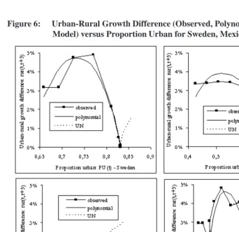
The Figure 6 illustrates for some countries – Sweden, Mexico, India, and China – how the polynomial model fits the historical trend (from left to right). The polynomial model adjusts thexuagainstPUbut the results are presented here asrurversusPUto facilitate
comparison between countries. The Figure also illustrates that the trend projected by the UN model (dotted curve) greatly departs from the trend projected by our model.
3.4 Corrections imposed on outliers
The Appendix 2 shows the importance of outliers identified after running the polynomial model. In this Appendix, the great outlying countries, for which we had to find specific solutions, are indicated. Other outliers were more easily dealt with and are also listed in the Appendix 2 along with the solution found to integrate them in the general model. We were not able to find any adjusting solution for only one small Caribbean island, Barbados (less than 270,000 inhabitants in 2000). For this country, we simply replicated the level of urbanisation attained in 1990, the year of the latest estimate, as the proportion urban did not vary much before.
Two cases are worth mentioning here. We had to run a specific model for Nigeria. In this country, hardly any data is available, except two unreliable censuses (1963 and 1991), to support any valuable projection on urbanisation. The projection using the standard polynomial model onxuproved unrealistic (leading to exponential urban growth from
2010: the proportion urban would reach about 80% in 2030 and would still increase after), because the population growth is probably overestimated for the whole country. Usingrur proved more realistic, but the projections thus obtained should not be taken
as very reliable either and are reported in the tables for the sake of offering a reasonable estimate for West Africa and for Africa as a whole. Another exception is Aruba Island in the Caribbean for which we run a simple regression model ofxuonPU, without the PU
2
component. Again, the projection should not be considered as very reliable for this country.
thorities instead, i.e. with no consideration of the size of the towns and of their limits. This undocumented change of definition led the UN to increase the estimates of the level of urbanisation at earlier dates (1995, 1990 and even 1985). Our correction for Kenya consisted in estimating the level of urbanisation in 1990 as per the published 1989 Cen-sus results and in discarding the UN estimates for 1995 and 2000. For Senegal, we used the latest 2002 Census results (not considered in the UN report) to estimate the level of urbanisation in 1990, 1995 and 2000, as the previous census was done long ago in 1987.
A last special case is with Colombia. In this country, the estimates for 1980 and 1985 looked inconsistent with the historical trend before 1980 and after 1985. We simply deleted those two observation points and found projections more compatible with the estimates for the years 1990 to 2000.
We had to adjust the model for 64 (i.e. 28%) out of 228 countries or territories of the UN database. The adjusted countries represent 43.2% of the world population en 2000 and China alone 21.0%. The adjustments were important in Southern Africa (affecting the estimates for 94% of the population of this region), Eastern Asia (86%, represent-ing China only), South Eastern Asia (77%), Western Africa (73%), Western Asia (62%), Western Europe (54%), Eastern Africa (36%) and Micronesia (32%). Two third of the adjustments (representing 30.8% of the world population) involved the removal of some early estimation of urbanisation, mostly the 1950s and 1960s estimates, i.e. applying the polynomial model on the most recent data. These corrections originate in absence of national data (i.e. estimation by the UN), poor quality of national data or in changes of definition of urban areas. The adjustments consisted for the remaining one third of correction cases (representing 12.4% of the world population) in removing the latest es-timations that appeared inconsistent with historical trends. This is where the adjustments are the most debatable. We would of course prefer to use recent estimates as they are supposed to reflect better the current level of urbanisation. However the latest estimates are subjected to definitional changes as much as the earliest estimates. Kenya is a good example where a change of definition led to an unexpectedly high growth in urban ar-eas. Because the author happened to live in Kenya at the time of writing, he was able to identify the definitional problem and make the necessary corrections. But certainly similar problems may arise for other countries identified as outliers, though it is not in the capacity of the author to document them all. For ease of interpretation of the results, the Appendix 2 is offering a correction score attached to the estimates depending on the extent of the corrections made on each outlier (score 1 for mild correction to score 5 for severe correction). A detailed examination of the countries identified as outliers is needed to produce better projection estimates in the future.
es-timates, from 1950 but no later than 1975, were removed), i.e. excluding the serious outliers with a correction score greater than 2 (see Appendix 2). Despite the variety of the definition of urban areas across countries and its occasional change over time in some countries, the results are certainly confirming the overall validity of the urban transition model for the estimation period. The complete urban projections up to 2030, by country and by regions, are available on the website http://www.demographic-research.org/, under the entry for publication 12-9 as an additional file in Excel format.
4. A comparison of the results obtained through the UN and the
poly-nomial models of projection
To confirm the validity of the model for the projection period, one needs to wait until estimates are produced for the year 2000 and more on the basis of country data. However it is possible to anticipate on the validity of the model in two ways, following the method proposed by N. Keyfitz (1981):
On past periods, by comparing the discrepancy measured by the Mean Percentage
Error (MPE) between the projections of the urban population obtained from the polynomial model from truncated data (e.g. 1950-1980) and the urban population as estimated by the UN (in 2000, for a 20-years projection period). We can then compare the results with the performance of the UN model over the same period. To assess this performance, we rely on the estimate of the MPE computed by B. Cohen (2004) by comparison of the projection made in the 1980 UN report with the estimates for 2000 made in the 2001 UN report, for 169 countries. For the sake of comparison with Cohen’s analyses, we also computed the Mean Absolute Percentage Error (MAPE) measuring the imprecision of the forecasts.
On future period, by comparing the MPE of UN past projections with the Mean
Percentage Difference (MPD) between UN future projections and the projections obtained from the polynomial model. If the UN model is overestimating the urban population in the same proportion for past and future forecasts and if the polyno-mial model better fits the historical trend, then the MPE and the MPD should give comparable results.
MAPE is high (27.0%) showing more imprecision than the UN projections (20.6%)4.
Removing 27 outliers (countries for which the projection of urban population was more than 1.5 times less or more than the estimation for the year 2000) improves considerably the precision, the estimate for the whole world becoming almost exact (MPE = 0.0%) with an imprecision divided by three (MAPE = 9.1%).
Table 1: Mean Percentage Error (MPE) and Mean Absolute Percentage Error (MAPE) in urban population polynomial projections by comparison with UN estimate for 2000 by level of development, size of the country and continent
MPE MAPE
Major Area or region 1980-2000 1980-2000 Number of (20-year projection) (20-year projection) countries
WORLD -1.1 % 27.0 % 209
World after eliminating 27 outliers 0.0 % 9.1 % 182
More developed countries 0.4 % 6.0 % 54
Less developed countries -1.4 % 32.1 % 155 LDC after eliminating 24 outliers -0.2 % 10.4 % 131 Size of the country:
0-2 million 2.1 % 26.8 % 76
2-10 million 5.8 % 19.1 % 59
10-50 million 14.9 % 27.9 % 54
50+ million -6.2 % 27.3 % 20
Continent:
Africa -3.7 % 23.3 % 51
Africa after eliminating 8 outliers -8.3 % 16.0 % 43
Asia -1.8 % 36.4 % 45
Asia after eliminating 6 outliers 2.3 % 9.1 % 39
Europe 4.2 % 6.6 % 46
South America 4.3 % 8.6 % 41
North America -6.3 % 6.3 % 5
Oceania -4.0 % 4.6 % 21
Source: our own computation by comparison of the projections obtained by the polynomial model with the UN estimation for 2000. MPE and MAPE are weighted by population size in 2000. Outliers are defined here as countries for which the projection of urban population was more than 1.5 times less or more than the estimation for the year 2000.
Countries 0% or 100% over the projection period are excluded from the computation.
4Part of this difference might be attributed to the choice of countries: Cohen used 169 countries “whose
boundaries have not change substantially” over the period while we used the whole UN data set on 209
The fit is actually better for MDC (MPE = 0.4%, MAPE = 6.0%) than for LDC (MPE = -1.5%, MAPE = 32.1%). The error in the projection is attributed mainly to some LDC. Removing 24 outliers (including China and Indonesia, two big outliers) from the compu-tation improves considerably the fit for LDC (MPE = -0.2%, MAPE = 10.4%). Africa and Asia show much higher variations (MAPE = 23.3% and 36.4% respectively) than other parts of the world (MAPE varying from 4.6% to 8.6%). Here again removing outliers improves the projections a lot (reducing the MAPE to 16.0% and 9.1% respectively for Africa and Asia). This is an indication that the quality of the data on urbanisation greatly affects the precision of the projections, a conclusion that converges with Cohen’s analysis of the bias in UN projections (Cohen 2004, p47).
The performance of the UN model over the past period 1980-2000, as measured by Cohen, is compared in Table 3 to the MPD measuring the difference between the UN projections and the polynomial projections for the 1995-2015 period. The Table 2 con-tains the detailed MPD by region of the world while the Table 3 compares the MPE and the MPD by country size for the 20-year projection period. Note that Cohen computed the MPE using the 2000 estimates from the 2001 UN report, nicknamed “ ’actual’ data” in his paper, which are not totally based on country data since not all countries had data available for this date. Even the 2003 UN report considers the 1995 data to be mostly based on country data whereas the 2000 estimates are said to be a mix of estimates and projections. Therefore for our computation of MPD, we considered the UN projections to be based on data up to 1995: the 20-year projection is for 2015 and the 35 year projection is for 2030. The 20-year projection period seems more reasonable to compare Cohen’s MPE and our own measure of MPD as the bias in measuring MPE will be minored by the difference due to the UN projection method.
The MPE is closer to zero in the polynomial projections (-1.1%, see Table 1) than it is in the UN projections (14.1%, see Table 3). The polynomial model would have performed much better on average than the UN model over the same period and using almost5the
same data. Also, the polynomial projections do not appear so biased for the LDC (MPE = -1.4%), contrary to the UN projections, which are higher in low income countries (MPE = 23.1%), and in lower middle income countries (MPE = 6.9%, but 25.6% when excluding China) and in upper middle income countries (MPE = 12.8%), compared to ‘only’ 6% in high income countries (Cohen 2004, Table 4)6.
If the polynomial model better fits the historical trend than the UN model, then the MPE for the past and MPD for the future should have comparable values, though the projections started from lower level of urbanisation in the case of MPE. The distribution of MPE and MPD are indeed strikingly similar for the 20-year projection period (Table 3).
5See note 4
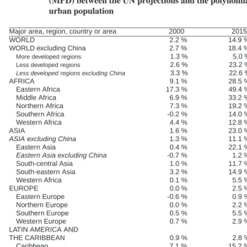
Table 2: Bias of UN model as measured by the Mean Percentage Difference (MPD) between the UN projections and the polynomial projections of urban population
Major area, region, country or area 2000 2015 2030
WORLD 2.2 % 14.9 % 34.5 %
WORLD excluding China 2.7 % 18.4 % 42.0 %
More developed regions 1.3 % 5.0 % 10.5 %
Less developed regions 2.6 % 23.2 % 51.0 %
Less developed regions excluding China 3.3 % 22.6 % 50.7 %
AFRICA 9.1 % 28.5 % 52.6 %
Eastern Africa 17.3 % 49.4 % 81.6 %
Middle Africa 6.9 % 33.2 % 66.0 %
Northern Africa 7.3 % 19.2 % 36.8 %
Southern Africa -0.2 % 14.0 % 29.0 %
Western Africa 4.4 % 12.8 % 28.0 %
ASIA 1.6 % 23.0 % 55.6 %
ASIA excluding China 1.3 % 11.1 % 33.7 %
Eastern Asia 0.4 % 22.1 % 46.4 %
Eastern Asia excluding China -0.7 % 1.2 % 7.7 %
South-central Asia 1.0 % 11.7 % 38.7 %
South-eastern Asia 3.2 % 14.9 % 33.4 %
Western Africa 0.1 % 5.5 % 16.9 %
EUROPE 0.0 % 2.5 % 8.0 %
Eastern Europe -0.6 % 0.9 % 7.0 %
Northern Europe 0.0 % 2.2 % 5.6 %
Southern Europe 0.5 % 5.5 % 14.6 %
Western Europe 0.7 % 2.9 % 5.7 %
LATIN AMERICA AND
THE CARIBBEAN 0.9 % 2.8 % 4.9 %
Caribbean 7.1 % 15.2 % 26.4 %
Central America 1.1 % 4.8 % 11.3 %
South America 0.2 % 0.7 % 0.2 %
NORTHERN AMERICA 4.8 % 10.8 % 15.2 %
OCEANIA 1.3 % 7.1 % 20.4 %
Australia/New Zealand 1.4 % 4.6 % 5.4 %
Melanesia 1.0 % 13.7 % 56.5 %
Micronesia 3.5 % 16.4 % 27.8 %
Polynesia -0.8 % 3.2 % 22.0 %
Less Developed Oceania 1.0 % 13.2 % 52.7 %
Source: our own computation by comparison of the UN projections and the polynomial regression model. MPD is
Table 3: Bias of UN projections as measured by the Mean Percentage Error (MPE) and the Mean Percentage Difference (MPD) in urban population projections
MPE MPD MPD
Major Area or region 1980-2000 1995-2015 1995-2030 (20-year projection) (20-year projection) (35-year projection)
WORLD 14.1 % 14.9 % 34.5 %
WORLD exluding China 19.0 % 18.4 % 42.0 %
Size of the country:
0-2 million 7.4 % 10.4 % 33.8 %
2-10 million 12.0 % 11.8 % 22.0 %
10-50 million 21.6 % 22.3 % 42.2 %
50+ million 12.4 % 13.1 % 33.4 %
50+ million exluding China 18.9 % 17.7 % 43.5 %
Source MPE: Table 4, Cohen (2004). 20 years: comparison of projection in 1991 UN report with estimates for 2000 as per 2001 UN report (169 countries).
Source MPD: our own computation by comparison of the projections obtained by the UN model and by the polynomial regression model (228 countries).
MPE is weighted by population size in 2000 whereas MPD is weighted by projected population size.
The overestimation of the urban population by the UN over the 1980-2000 period seems to replicate almost identically for the 1995-2015 period, for all country size, and looks worse when we exclude China. The difference between the UN model and the polynomial model is very high for the whole of Africa and for Eastern Africa and Middle Africa in particular. The difference is also substantial in Eastern Asia (mainly because of China), in South-Central Asia and South-Eastern Asia, as well as in the Caribbean, Melanesia and Micronesia. All these regions are notoriously less developed, but the difference is also observed for more developed regions such as Northern America. The fact that the analysis of the bias of UN projection tallies very closely with the analysis of the difference between the UN projection and our own projection seems to indicate that the polynomial model is well suited for projecting the historical urban trends. But of course, only the future will tell if our projections were right.
countries, United States of America are the main contributor to the difference in the world estimation (4.5%).
Obviously any projection will be sensitive to the estimation in these countries, which are also among the most populous in the world. Because they concentrate a large share of the world population, China (1.28 billion inhabitants in 2000, 1.45 projected in 2030) and India (1.02 billion in 2000, 1.42 in 2030) are of particular concern regarding urbanization. In the case of China, the Cultural Revolution led to a sharp slow-down in the late 1960s followed by a sharp rise in the urban growth in the late 1970s (Liang 2001). However our projections, which discarded the data prior to 1970, predict that the urban growth should start to decline at the end of the 20th century and that the proportion urban in China should stabilize at less than 40% from 2030. This departs largely from the UN projections predicting figures of 35.8% in 2000 and 60.5% in 2030, as illustrated in Figure 6. In our projection, the stabilization of the proportion urban at what would seem a low level is partly due to the definition of urban areas. China is using a very high threshold (100,000 inhabitants) combined with population density criteria together with a complex functionalist definition of smaller urban agglomeration using various criteria (majority of non-agriculture activities, percentage use of water, industrial output, GDP, etc.). To add on the difficulty, these criteria evolved significantly since the 1980s (Zhu 2003). The UN series up to 1995 seems to be consistent with the 1990 definition. The last, more internationally accepted change of definition was implemented in 2000 with the effect of increasing by about 6 points the level of urbanization, estimated at 36.1% in 2000, as compared to 30.9% in 1999. Using an even more standard definition of urban areas (e.g. agglomerations of 10,000 inhabitants or more) would obviously lead to a much higher level of urbanization, maybe adding up 10 percentage points to the figures published with the 1990 definition, which would make China 50% urban by the year 2030 according to our projection trends (instead of 40% using the 1990 definition).
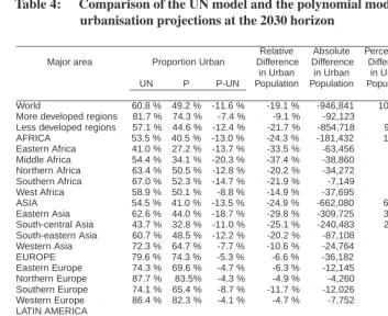
Table 4: Comparison of the UN model and the polynomial model (P) for urbanisation projections at the 2030 horizon
Relative Absolute Percentage Urban-Rural
Major area Proportion Urban Difference Difference Difference Growth
in Urban in Urban in Urban Difference
UN P P-UN Population Population Population (2025-2030)
UN P
World 60.8 % 49.2 % -11.6 % -19.1 % -946,841 100.0 % 2.08 % 0.13 %
More developed regions 81.7 % 74.3 % -7.4 % -9.1 % -92,123 9.7 % 1.93 % 0.16 %
Less developed regions 57.1 % 44.6 % -12.4 % -21.7 % -854,718 90.3 % 2.32 % 0.29 %
AFRICA 53.5 % 40.5 % -13.0 % -24.3 % -181,432 19.2 % 2.31 % 0.45 %
Eastern Africa 41.0 % 27.2 % -13.7 % -33.5 % -63,456 6.7 % 2.52 % 0.85 %
Middle Africa 54.4 % 34.1 % -20.3 % -37.4 % -38,860 4.1 % 2.80 % -0.02 %
Northern Africa 63.4 % 50.5 % -12.8 % -20.2 % -34,272 3.6 % 2.43 % 0.33%
Southern Africa 67.0 % 52.3 % -14.7 % -21.9 % -7,149 0.8 % 2.23 % 0.09 %
West Africa 58.9 % 50.1 % -8.8 % -14.9 % -37,695 4.0 % 2.41 % 0.83 %
ASIA 54.5 % 41.0 % -13.5 % -24.9 % -662,080 69.9 % 2.49 % 0.20 %
Eastern Asia 62.6 % 44.0 % -18.7 % -29.8 % -309,725 32.7 % 2.58 % 0.00 %
South-central Asia 43.7 % 32.8 % -11.0 % -25.1 % -240,483 25.4 % 2.93 % 0.35 %
South-eastern Asia 60.7 % 48.5 % -12.2 % -20.2 % -87,108 9.2 % 2.56 % 0.54 %
Western Asia 72.3 % 64.7 % -7.7 % -10.6 % -24,764 2.6 % 1.58 % -0.17 %
EUROPE 79.6 % 74.3 % -5.3 % -6.6 % -36,182 3.8 % 1.84 % 0.21 %
Eastern Europe 74.3 % 69.6 % -4.7 % -6.3 % -12,145 1.3 % 1.69 % 0.01 %
Northern Europe 87.7 % 83.5% -4.3 % -4.9 % -4,260 0.4 % 1.71 % 0.11 %
Southern Europe 74.1 % 65.4 % -8.7 % -11.7 % -12,026 1.3 % 2.03 % 0.01 %
Western Europe 86.4 % 82.3 % -4.1 % -4.7 % -7,752 0.8 % 1.68 % 0.43 %
LATIN AMERICA
and CARIBBEAN 84.6 % 82.1 % -2.0 % -3.0 % -17,976 1.9 % 1.67 % 1.08 %
Caribbean 73.3 % 60.4 % -12.9 % -17.6 % -5,857 0.6 % 1.87 % -0.06 %
Central America 77.5 % 70.9 % -6.6 % -8.5 % -12,730 1.3 % 1.82 % 0.21 %
South America 88.6 % 88.8 % 0.1 % 0.1 % 611 -0.1 % 1.60 % 2.13 %
NORTHERN AMERICA 86.9 % 75.4 % -11.4 % -13.2 % -46,611 4.9 % 1.70 % -0.01 %
OCEANIA 74.9 % 68.7 % -6.2 % -8.2 % -2,560 0.3 % 0.48 % -0.50 %
Australia/New Zealand 94.9 % 90.0 % -4.9 % -5.1 % -1,375 0.1 % 1.45 % 0.35 %
Melanesia 27.2 % 18.2 % -9.0 % -33.2 % -1,046 0.1 % 2.65 % -0.24 %
Micronesia 81.2 % 70.0 % -11.2 % -13.8 % -84 0.0 % 1.85 % 0.09 %
Polynesia 55.0 % 48.4 % -6.5 % -11.9 % -55 0.0 % 2.36 % 0.34 %
Less Developed Oceania 32.0 % 23.0 % -9.0 % -28.1 % -1,184 0.1 % 2.27 % -0.18 %
estimates and projections for China and Asia as a whole.
We don’t expect the same definitional problem with India because this country uses a much lower threshold (5,000 inhabitants), together with a functionalist approach (ad-ministrative centers, non-agricultural activities). According to our projections (illustrated in Figure 6), the level of urbanization in India would hardly reach 31% in 2030. This compares with 41.4% in the UN projection for 2030 but with persistent growth after this date. Here the difference in estimation is mainly attributed to the difference in modeling. If the polynomial model proved right, the majority of the developing world would not live in urban areas by 2030. The population would stay predominantly rural in Africa and in Asia (Table 4). Even more importantly, the potential for future urban growth is very much reduced in the projections based on the polynomial model. As an indication of this potential, the urban-rural growth difference (rur) for the period 2025-2030 is reported
in Table 4. In the UN projections therurranges in each region between 1.5% and 3%
whereas in the polynomial projections therurhovers around 0% and exceeds 2% only
in South America, while it is sometimes negative (as in Western Asia and Melanesia), indicating reverse urbanisation.
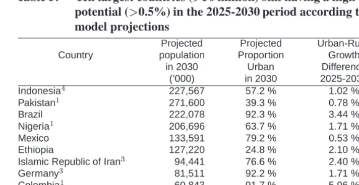
The UN methodology used for projection inevitably forecasts that the proportion ur-ban would one day reach 100%. On the contrary, the polynomial model indicates that urban saturation could be attained not long after 2030. Therefore, there is a huge dis-crepancy between the UN projections and our projections based on the historical patterns of urban transition. According to the polynomial model, very few countries would still have in 2030 a high potential for urban growth. The Table 5 indicates the most populous countries (with 50 million inhabitants or more in 2030) which would still have a highrur
(more than 0.5% a year in the 2025-2030 period). Quality of the projections notwithstand-ing (six of them were subjected to special corrections before projections, see Appendix 2), those large, mostly developing countries7representing 18.8% of the world population in 2030 would account for 38.1% of the urban population increase between 2025 and 2030. India with arurof only 0.26% a year would account for 12.3% of the world urban
pop-ulation increase. To summarize, ten developing countries would contribute to more than half of the world urban population increase in the 2025-2030 period. Many of the remain-ing countries would have reached their urban saturation level, contributremain-ing marginally to the world urban growth after 2030.
5. Conclusions: improving projection models
It is clear from our analysis that the UN projections are biased and lead to a gross over-estimation of urbanization trends. Contrary to the common belief, the UN projections are
Table 5: Ten largest countries (>50 million) still having a high urban growth potential (>0.5%) in the 2025-2030 period according to the polynomial model projections
Projected Projected Urban-Rural Additional Country population Proportion Growth urban
in 2030 Urban Difference population (’000) in 2030 2025-2030 2025-2030 Indonesia4
227,567 57.2 % 1.02 % 7,630
Pakistan1
271,600 39.3 % 0.78 % 10,906
Brazil 222,078 92.3 % 3.44 % 8,126
Nigeria1 206,696 63.7 % 1.71 % 13,117
Mexico 133,591 79.2 % 0.53 % 3,519
Ethiopia 127,220 24.8 % 2.10 % 4,995
Islamic Republic of Iran3
94,441 76.6 % 2.40 % 4,710
Germany3
81,511 92.2 % 1.71 % 110
Colombia1
60,843 91.7 % 5.96 % 3,952
Republic of Korea 50,042 90.2 % 0.85 % 79
Total 10 countries 1,525,588 - - 57,144
China 1,450,521 39.8 % 0.02 % 2,554
India 1,416,576 30.9 % 0.26 % 18,432
World 8,130,149 49.2 % 0.13 % 149,974
Note: Countries subjected to corrections in the polynomial model are indicated by their correction score: 1 (mild correction), 3 (high correction), 4 (very high correction). The projections for those countries are therefore to be cautiously interpreted.
not based on the extrapolation of historical trends. We proved that this can be attributed mainly to an inappropriate projection model that systematically biases the urban estimates upward, and also to the quality of the available data. The fairly simple polynomial model that we propose here as an alternative captures most of the historical trends (as reported by the UN) and projects them well in the future, country by country. We hope that the results presented here will extend the debate and that other models will be proposed to the users of world urban population projections. In particular, we should compare the results of the projections using the UN data with the multiregional projections obtained using more complex models (Rogers 1995) capable of offering better results albeit with more detailed data. Meanwhile, the polynomial model of urban transition has limitations that should be taken into account to refine the projections:
Our projections are based on the World Urbanization Prospects published by the
Results show that the information on urbanisation is better used at a country level
than at a sub-regional level or continental level. An improvement would be to work at a sub-country level for such countries as China, India, etc., where there are huge discrepancies between provinces or States.
Particular effort should be devoted at finding better estimations for the countries for
which we had to make specific corrections. In these countries the problem is more with the data that form the base for projection than with the model itself.
International comparisons become difficult when countries are using very different
urban definitions. Coordination is needed to evaluate the population in urban areas according to an internationally recognised definition. An alternative to the projec-tion of the overall urban populaprojec-tion would be the projecprojec-tion of the urban populaprojec-tion above high thresholds (e.g. agglomerations of more than 20,000, 50,000, 100,000 or 500,000 inhabitants) that could easily be computed using a list of towns and cities ranked by size in each country. A model relating the estimates obtained at each threshold could then be used to evaluate a standard urbanisation rate at a lower threshold (e.g. 10,000 inhabitants).
To improve the projections, it is however clear that the available data set is not satisfac-tory. As earlier recommended by an international panel of scientists (National Research Council 2003), considering the importance of urban projections for demographers and ge-ographers, and also for other scientists and policy makers, the UN’s Population Division would give everyone a great service in making the original data set available to the public so that projections and data from each country are put under the scrutiny they deserve by the scientific community.
6. Acknowledgements
References
Bairoch, P. (1985). De J ´ericho `a Mexico : villes et ´economie dans l’histoire. Paris: Gallimard.
Balk, D., F. Pozzi, G. Yetman, A. Nelson, and U. Deichmann. (2004). Methodologies to improve global population estimates in urban and rural areas. Presented at 68th Annual Meeting of the Population Association of America, April 1-3, 2004, Boston MA, USA.
Champion, A.G. (1989). Counterurbanization - The Changing Pace and Nature of Population Deconcentration. London: Edward Arnold.
Champion, T. (1989). Urbanization, suburbanization, counterurbanization and reurban-ization. Handbook of Urban Studies, edited by R. Paddison. London: Sage Publi-cations Ltd, 143-161.
Chandler, T. (1987). Four Thansand Years of Urban Growth: An Historical Census. Lampeter, Dyfed: Edwin Mellen Press.
Cohen, B. (2004). Urban growth in developing countries: A review of current trends and a caution regarding existing forecasts. World Development, 32(1), 23-51.
Davis, J.C. and J.V. Henderson. (2003). Evidence on the political economy of the urban-ization process. Journal of Urban Economics, 53, 98-125.
de Vries, J. (1984). Urban growth in developing countries: A review of current trends and a caution regarding existing forecasts. European Urbanization, 1500-1800, London: Methuen.
EIA. (2004). International Energy Outlook. Washington, D.C.: Energy Information Administration.
Hugo, G. and A. Champion. (2003). New Forms of Urbanisation. Aldershot: Ashgate.
IEA. (2004). World Energy Outlook. Paris, France: International Energy Agency.
Keyfitz, N. (1980). Do cities grow by natural increase or by migration? Geographical Analysis, 12(2), 142-156.
Liang, Z. (2001). The age of migration in china. Population and Development Review, 27(3), 499-524.
Moriconi-Ebrard, F. (1993). L’urbanisation du monde depuis 1950. Paris: Anthropos.
Moriconi-Ebrard, F. (1994). GEOPOLIS - Pour comparer les villes du monde. Paris: Anthropos.
National Research Council. (2003). Cities transformed - demographic change and its implications in the developing world. edited by National Research Council. Wash-ington D.C.: The National Academies Press, Pp. 529.
Njoh, A.J. (2003). Urbanization and development in sub-saharan africa. Cities, 20(3), 167-174.
Rogers, A. (1995). Multiregional Demography - Principles, Methods and Extensions. Chichester: John Wiley & Sons.
UN-Habitat. (2003). Slums of the world: The face of urban poverty in the new millenium? monitoring the millenium development goal, target 11 - world-wide slum: Dweller estimation. Nairobi: UN-Habitat.
UNDP, UNEP, World Bank, and World Resources Institute. (2003). World Resources 2002-2004: Decisions for the Earth: Balance, voice, and power. Washington, D.C.: United Nations Development Programme, United Nations Environment Pro-gramme, World Bank, World Resources Institute.
United Nations. (1997). World urbanization prospects: The 1996 revision. New York: United Nations Secretariat, Population Division.
United Nations. (2002). World urbanization prospects: The 2001 revision. data tables and highlights. New York: United Nations Secretariat, Population Division.
Woods, R. (2003). Urbanisation in europe and china during the second millenium: A review of urbanism and demography. International Journal of Population Geogra-phy, 9(3), 215-227.
World Bank. (2003). Global Economic Prospects and the Developing Countries 2004. Washington, D.C.: World Bank.
Zelinsky, W. (1983). The impasse in migration theory: a sketch map for potential es-capees. Population movements : their forms and functions in urbanization and development, edited by P.A. Morrison. Li`ege: Ordina - IUSSP, 19-46.
Appendix I
The relation between the Urban-Rural Growth Difference (rur) and the Excess In-crease in Urban Areas (xu)
Andrei Rogers (1995) noted that the urban-rural growth difference can be expressed using the migration and natural increases in urban and rural areas:8
rur t =u t r t =(n u m u;r + R t 1 U t 1 m r;u ) (n r m r;u + U t 1 R t 1 m u;r ) (1)
where all rates are computed in term of the population at timet 1:
natural rate in the urban population:
n u = N u U t 1
natural rate in the rural population:
n r = N r R t 1
migration rate from urban to rural areas, expressed per urban resident:
m u;r = M u;r U t 1
migration rate from rural to urban areas, expressed per rural resident:
m r;u = M r;u R t 1
whereNandMstand respectively for the natural and the migration increase.
Separating in equation (1) the natural rates from the migration rates and expanding gives: rur t = N u U t 1 N r R t 1 + M r;u R t 1 R t 1 U t 1 +1 M u;r U t 1 U t 1 R t 1 +1 = N u U t 1 N r R t 1 + M r;u U t 1 +R t 1 U t 1 R t 1 M u;r U t 1 +R t 1 U t 1 R t 1
8For convenience of demonstration, we will consider a one-year interval. The demonstration can easily be
In this last expression ofrur, one notices that apart from the natural and migration
in-creases, the right-hand side of the equation makes a repeated use of the population urban and rural known from the preceding periodt 1. It is actually possible to simplify the
equation by extracting from the righ-hand side the term U t 1 +R t 1 Ut 1Rt 1 : rur t = U t 1 +R t 1 U t 1 R t 1 + R t 1 U t 1 +R t 1 N u U t 1 U t 1 +R t 1 N r +M r;u M u;r rur t = U t 1 +R t 1 U t 1 R t 1 + + N u U t 1 U t 1 +R t 1 (N r +N u
)+M r;u
M u;r
(2)
By noticing that
Ut 1 Ut 1+Rt 1 (N r +N u
)is simply the theoretical natural increase in
urban areas if urban areas were to grow at the same natural rate than the total population, we can rearrange equation (2) so that:
rur t U t 1 R t 1 U t 1 +R t 1 =N u U t 1 U t 1 +R t 1 (N r +N u
)+M r;u
M u;r (3)
which is to be interpreted as, in the interval (t 1;t):
excess increase inU =excess natural increase inU+excess migration increase inU
The left-hand side of equation (3) now contains only known quantities based on the population estimates in urban and rural areas, whereas the right – hand side now contains unknown (to the urbanisation database) quantities – natural and migration balances.
We can verify that the left-hand side of equation (3) represents well the excess increase in urban areas by remembering that:
and rearranging from equation (3): rur t U t 1 R t 1 U t 1 +R t 1 = U t U t 1 U t 1 R t R t 1 R t 1 U t 1 R t 1 U t 1 +R t 1 = (U t R t 1 R t U t 1 ) 1 U t 1 +R t 1 = U t (U t 1 +R t 1 ) U t 1 (U t +R t ) U t 1 +R t 1
we finally obtain the excess total increase in urban areasxu:
xu t =rur t U t 1 R t 1 U t 1 +R t 1 =U t U t 1 U t +R t U t 1 +R t 1 =U t U t 1 p t (4) wherep
tis the total growth rate of the population and U
t 1 p
tthe hypothetical absolute