Print ISSN: 2383-451X Online ISSN: 2383-4501 Web Page: https://jpoll.ut.ac.ir, Email: [email protected]
Study of Solute Dispersion with Source/Sink Impact in
Semi-Infinite Porous Medium
Kumar, R.1, Chatterjee, A2., Singh, M. K.1* and Singh, V. P.3
1. Department of Mathematics and Computing, Indian Institute of Technology (Indian School of Mines), Dhanbad-826004, Jharkhand, India
2. Department of Mathematics, The Neotia University, Diamond Harbour, West Bengal, India
3. Department of Biological and Agricultural Engineering & Zachry Department Civil Engineering, Texas A and M University, 321 Scoates Hall, 2117 TAMU,
College Station Texas 77843-2117 USA
Received: 25.07.2019 Accepted: 19.11.2019
ABSTRACT: Mathematical models for pollutant transport in semi-infinite aquifers are based on the advection-dispersion equation (ADE) and its variants. This study employs the ADE incorporating time-dependent dispersion and velocity and space-time dependent source and sink, expressed by one function. The dispersion theory allows mechanical dispersion to be directly proportional to seepage velocity. Initially the aquifer is assumed contaminant free and an additional source term is considered at the inlet boundary. A flux type boundary condition is considered in the semi-infinite part of the domain. Laplace transform technique (LTT) is then applied to obtain a closed form analytical solution. The effect of source/sink term as a function in the one-dimensional advection-dispersion equation is explained through the graphical representation for the set of input data based on similar data available in hydrological literature. Matlab software is used to obtain the graphical representation of the obtained solution. The obtained analytical solution of the proposed model may be helpful in the groundwater hydrology areas.
Keywords: Aquifer; Advection; dispersion; Contamination; Source-Sink.
INTRODUCTION
Groundwater is a vital source of drinking water and agricultural irrigation in rural India. Unfortunately, groundwater has become highly polluted by municipal, commercial, residential, industrial, and agricultural activities. Examples include chemical fertilization, industrial waste storage or spills, hospital wastes, leakage from petrol pumps, septic systems, and wells. The literature on point and non-point source pollutant transport groundwater is
*
Corresponding Author, Email: [email protected]
damage of the system in a waste material depository or sewage sludge (Balla et al., 2002). Also, the periodic type boundary conditions were employed in a semi-infinite domain to obtain the solutions for ADE (Logan & Zlotnik, 1995). However, a solution of the ADE was developed to describe chemical transport with sorption and decay in a finite domain (Golz & Dorroh, 2001). An analytical solution was also presented for solute transport in rivers considering transient storage with instantaneous injection (Smedt et al., 2005). For a finite spatial domain, the 1-D ADE with an arbitrary time-dependent inlet boundary condition was solved analytically using LTT and Generalize Integral Transform Technique (GITT) (Chen & Liu, 2011). Also, Green’s function method was adopted to develop the analytical solution of ADE for steady 1 or 2-D flow in homogeneous porous media (Leij et al., 2000). Two different types of boundary conditions (Dirichlet and Cauchy) were used to obtain a general solution for a 1-D reactive transport model (Srinivasan & Clement, 2008). In the groundwater system, the interpolation polynomial method was employed to derive the higher order schemes of advection–diffusion (Tkalich, 2006). Considering the dispersion coefficient as a time-dependent function in 2-D ADE, the analytical solutions were developed for two-point sources i) instantaneous and ii) continuous in an infinite aquifer (Aral & Liao, 1996). Using LTT, an analytical solution was obtained for the ADE with the help of longitudinal dispersion along unsteady groundwater flow in the finite part of aquifer and an explicit finite difference scheme was used to obtain numerical solution (Singh et al., 2015). After that, the depth dependent variable source was considered at the inlet location of the model domain to solve the 2-D ADE by finite element method (Chatterjee & Singh, 2018). Two problems were discussed in the semi-infinite aquifer with exponentially spatially
dependent initial condition under the specific assumptions i) temporal dependent velocity in the part of homogeneous medium and ii) spatially and temporal dependent velocity in the part of heterogeneous medium (Thakur et al., 2019). A numerical model was presented for the multispecies contaminant transport problem in the porous medium (Natarajan & Kumar, 2017). With constant concentration source and flux type boundary source in the horizontal and vertical medium, the solution was obtained analytically using LTT for transient water and contaminant transport (Sander & Braddock, 2005).
Two solutions were presented for a solute transport modelling under the specific assumption i) distance-dependence dispersion and ii) time-dependence source of contaminant in the finite column (You & Zhan, 2013). For a saturated semi-infinite porous media, a general analytical solution was obtained for an instantaneous contaminant point source by using the method of source function (Bai et al., 2015). A boundary layer theory was used on convection–dispersion equation, to obtain the general polynomial solution (Wang et al., 2017). Moreover, two models of 1-D ADE were developed, where in the first model the diffusion coefficient was assumed as constant and flow velocity was variable and in the other model both were variables. Semi-analytical solutions were developed using the Laplace transformation and also using a special approximation scheme to the variable flow velocity and diffusion coefficient (Jia et al., 2013). Most of these studies were employed 1-D with time and space dependent velocity and dispersion coefficient. But our main concern in this study is to incorporate the source/sink term with the ADE. There have limited studies in this context, and some of them are pointed out below.
et al., 1999). Also, the density profile was calculated for vertical source/sink of ammonia within-canopy by using the inverse Lagrangian technique (Nemitz et al., 2000). Furthermore, the analytical solutions were developed for steady-state and transient, consisting of parallel discrete fractures and evenly spaced in a porous medium. The solutions, obtained by using Laplace and Fourier transforms, contained longitudinal and transverse dispersion; a strip source of finite width, aqueous and source decay (West et al., 2004). However, the arsenic in groundwater due to high carbonates wetland soils was observed (Bauer et al., 2008). The constructed wetland facilities discussed using simulation of flow and nitrogen transformation through the ADE with linear sink-source terms in horizontal subsurface flow (HSF) (Moutsopoulos et al., 2011). But on the regional scale for substance flows the sinks were assessed (Kral et al., 2014). The nonlinear wind input term was used to discuss the wind wave interaction and white capping dissipation depending on the growth of airflow separation, wave steepness and negative growth rate under adverse winds (Zieger et al., 2015). The hydrodynamic dispersion coefficients were used to characterize in a gravel layer for the prediction of nonpoint source pollutant migration in alpine watersheds by using an electrolyte tracer method (Shi et al., 2016). Using an eco-hydrological watershed model, an improve water quality for an efficient watershed management plan was developed (Amin et al., 2017). An integrated approach was presented to predict the current and future climatic changes for flow and salt concentration in the system of groundwater which is linked by the soil and water application tool (SWAT), MODFLOW, and 3-D groundwater variable-density flow that were coupled with the multi-species solute and heat transport models (Akbarpour & Niksokhan, 2018).
The main focus of the present study therefore is to derive a closed form solution
of 1-D ADE with source and sink term incorporated for solute transport in an aquifer of semi-infinite. This study also included the space and time dependent source term expressed in a functional form that influences pollution concentration, as well as a sink term as a remedial measure using the same function after a certain distance. This type of work has not been reported yet. In all previous studies the source/sink terms were presented as a function of time or space, but in this study we considered source or sink term as a function of space and time dependence in the form, g x t( , )h t( ) ( ) x , where the time dependent part is measured in general form.
MATHEMATICAL FORMULATION The groundwater pollutant concentration is investigated with the effect of source/sink term, and represented by some space and time dependent functions. Because source/sink term represents pollutant added to or removed from the medium (i.e., positive for source and negative for sink). Solute movement in the flow region occurs due to advection and dispersion. A point-source pollutant significantly reflects the higher concentration in the groundwater system and the pollutant spreads in the flow direction of groundwater in the aquifer. In this study, the aquifer domain is assumed to be homogeneous and the one-dimensional solute movement is investigated analytically by using ADE with time-dependent dispersion and velocity and space-time dependent source and sink term, mathematically expressed by single function in the form, g x t( , )h t( ) ( ) x .
The 1-D ADE with source and sink in a semi-infinite aquifer can be written as:
2 1 0
2 ( , )
C C C
u D c g x t
t x x
(1)
where, C denotes the pollutant
source-sink term as a function of space
x
and timet
, i.e. g x t( , )h t( ) ( ) x .The time-dependent Dirichlet type source of contaminant is considered at the upper end of the aquifer, i.e. x0and the concentration gradient at the downstream end of the aquifer (at infinite distance) is assumed to be zero. Initially the aquifer is considered to be pollutant free. Thus, the initial and boundary conditions can be written as:( , ) 0, 0
C x t t (2)
0
( , ) ( ), 0
C x t c f t x (3)
0 C x x (4)
We consider that f t( )is an exponentially decreasing function of time
t
, i.e.,2
( ) exp( )
f t k t , where k2 is a constant. The dispersion is considered to be directly proportional to seepage velocity (Freeze & Cherry, 1979). Hence, the dispersion and seepage velocity were expressed as follows:
0
( )
u u h t
and DD h t0 ( ) (5)where D0 and
u
0 are the initial dispersion and seepage velocity coefficient, respectively; and h t( ) is considered as a exponentially decreasing function of timet
i.e., h t( )exp(k t1 ).Now we use the following
transformation:
* *
0
( )
t
T
h t dt (6)and express Eq. (1) as
2 1
0 0 2 0 ( )
C C C
u D c x
T x x
(7)
where,
0
( ) ( )x s x
s
is the non-dimensional
function and the space dependent function
is ( )
0
( ) x a
s x b e and
s
0 is the function value at x=0.To remove the advection term from the Eq. (7) by using the following transformation
2
0 0
0 0
( , ) ( , ) exp
2 4
u x u T
C x T K x T
D D
(8)
Substitution of Eq. (8) in Eq. (7), we obtain
2 2
1 0 0
0 2 0
0 0
exp ( )
4 2
u T u x
K K
D c x
T x D D
(9)
Now the initial condition becomes
( , ) 0 0
K x T T (10)
and the boundary conditions become
0
( , ) ( ) 0
K x T c T x (11)
0 0 0 2 u K K x x D (12)
DERIVATION OF ANALYTICAL SOLUTION
Taking the Laplace transform of Eq. (9), we obtain
1 2
0 0 2
0 2
0 1
exp( ( ))
( )
c b A x a K
D p K
x s p B
(13)
where, 0
2 0 1 2 u A D
and 20
1 0 4 u B D
Also, taking the Laplace transform of Eq. (11) and Eq. (12), we get
0 2
( , ) 0
( )
c
K x p x
p B (14) 0 0 0 2 u K K x x D (15)
where, B2 B1 k2.
With the use of the boundary conditions given by Eqs. (14)-(15), the solution of Eq.
(13) in terms of K x p( , )
1
0 0 0
2
2 0 0 1 2 0 0
1
0 0 2
2
0 1 2 0
exp( )
( , ) exp exp
( ) ( )( )
exp( ( ))
( )( )
c p c b a p
K x p x x
p B D s p B p A D D
c b A x a
s p B p A D
(16)
Taking inverse Laplace transform of Eq. (16), we obtain the solution is as follows:
1 1
0 0 0 0 2
0 1 2 2 2 3 4
0 1 2 0 0 1 2 0
exp( ) exp( ( ))
( , ) ( )
( ) ( )
c b a c b A x a
K x T c I I I I
s B A D s B A D
(17)
where,
2
2
1 1 1 1 1 1 1
1
exp exp
2 2 2
X X
I a T a X erfc a T a T a X erfc a T
T T
2
2
21 2 2 2 2 2 2
1
exp exp
2 2 2
X X
I a T a X erfc a T a T a X erfc a T
T T
2
2
22 3 3 3 3 3 3
1
exp exp
2 2 2
X X
I a T a X erfc a T a T a X erfc a T
T T
2 21 22
I I I ,
0
x X
D
, I3 exp
a T22 ,
2 4 exp 3
I a T a1 B2, a2 B1 and a3A2 D0 .
Substituting the value of K x T( , ) in the Eq. (8), we get the solution of the
considered model as:
1 1 2
0 0 0 0 2 0 0
0 1 2 2 2 3 4
0 1 2 0 0 1 2 0 0 0
exp( ) exp( ( ))
( , ) ( ) exp
( ) ( ) 2 4
c b a c b A x a u x u T
C x T c I I I I
s B A D s B A D D D
(18)
In the special case, the analytical solution is obtained in the absence of
source/sink function i.e., g0 in Eq. (1) is as follows:
2
1 1 1 2
0 0 0
0 0
2
1 1 1
exp
2
( , ) exp
2 2 4
exp
2
X
a T a X erfc a T T
c u x u T
C x T
D D
X
a T a X erfc a T T (19)
RESULT AND DISCUSSIONS
For the computation we considered
1
0 1.0 / ( * )
c mg l year , c01.0mg l/ , k10.1/year,
2 0.01/
k year, 2
0 0.05 /
D km year, u00.2km year/ , 0 0 0.5
a b km in the reasonable range from
the existing literature (Singh & Kumari, 2014). It was assumed that the source of contamination originated below the water table which may occur in many situations, such as materials stored or disposed by
deep well injection, agricultural drainage wells, and industrial disposal sites, to name but a few.
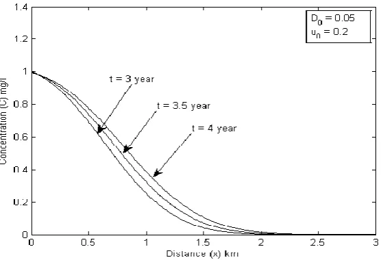
Fig. 1 plots the curves showing concentration in the aquifer at t = 3, 3.5
and 4 years. The contaminant
aquifer. The peak pollutant concentration moved from the additional source function; after x= 0.5 km the contaminant concentration decreased with distance and asymptotically approached zero. We observed form the Fig.1, the contaminant concentration increased sharply for all three different times at the inlet location of the modal domain. The concentration values is lower at each of the position in the aquifer as well as intermediate position
for the time period t = 3 year as compare to the long time period i.e., t = 3.5 and 4 years as shown in the Fig.1. Overall, we observed that the rate of increase of the pollutant concentration is slower for the small time period and the rate of decrease of the pollutant concentration is faster for the small time period along the flow direction as shown in the Fig.1 and towards the exit boundary.
Fig. 1. The pollutant concentration profile depicted for the solution of Eq. (18) with fixed dispersion and velocity at three different times.
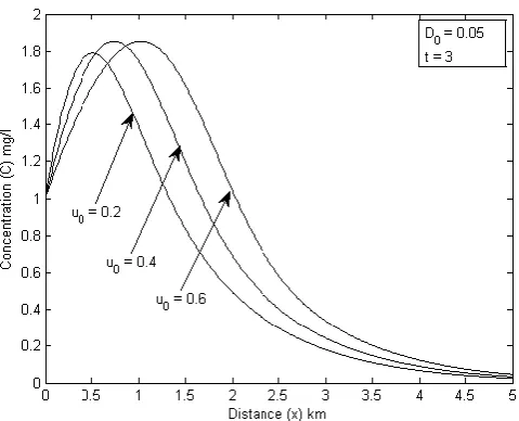
Fig. 3. The pollutant concentration profile depicted for the solution of Eq. (18) at three different velocities profiles with fixed dispersion and particular time.
Fig. 4. The pollutant concentration profile depicted for the solution of Eq. (18) at three different dispersions with fixed velocity and particular time.
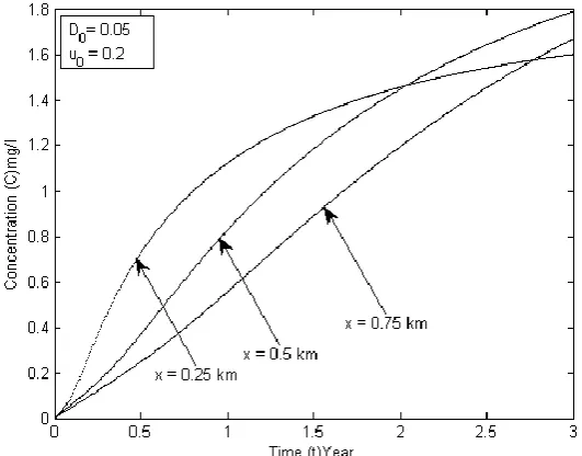
The pollutant concentration rapidly increases for all three fixed location in the aquifer with respect to time as shown in the Fig.2. From this Fig. we observed that the Pollutant concentration highly increased for the particular distance x = 0.25 km as compare to the other fixed distances x = 0.5 and 0.75 km from the beginning of the time i.e., 0 t 2 years after that time i.e., 2 t 2.7 years, the concentration values are higher for the fixed distance x = 0.5 km as compare to the fixed distance x = 0.25 km and 0.75 km.
location of the aquifer. For the distance 0 x 0.5 km, the concentration values are higher at each of the position for the low velocity profile other than high velocity profiles due to effect of the additional source function as shown in the Fig. 3 but after that distance i.e., 0.5 x 5km the concentration values are lower at each of the position as well as intermediate position in the aquifer domain for the low velocity profile as compare to the high velocity profiles and the peak contaminant concentration moved from additional function. Overall, it is quite clear that the rate of decrease of the pollutant concentration is faster for the low velocity profile along the flow direction as shown in the Fig.3.
The pollutant concentration profile is depicted for three different dispersion profiles with fixed velocity and particular time t = 3 year as shown in the Fig.4. From this Fig. it is clearly observed that the concentration values start from the inlet location of the aquifer domain and sharply increased from 0 x 0.5 km because of additional source function but the peak pollutant concentration moved from one source function, after x0.5 km the pollutant concentration decreases when distance increases and tends to zero for all different dispersion profiles. For the fixed
dispersion coefficient D0=0.05 km2/year, the concentration values are higher at each of the position for this domain i.e., 0 x 1 km but for the fixed dispersion coefficient
D0=0.07 km2/year, the concentration values are higher from the fixed dispersion D0=0.09 km2/year at each of the position for this domain i.e., 0 x 1 km but lower from the dispersion coefficient D0=0.05 km2/year. But after that distance 1 x 3 km, the pollutant concentration values for the dispersion coefficient D0=0.07 km2/year are higher from D0=0.09 km2/year and lower from D0=0.05 km2/year at each of the position for the same domain as shown in the Fig. 4. Overall, the peak pollutant concentration for all three profiles moved from one additional source function and decreases towards the exit boundary.
The three depicted Figs. 1, 3 and 4, clearly indicate that the effect of source-sink term in the aquifer domain. The contaminant concentration initially starts from the input value i.e., x = 0 in the aquifer and exponentially increased with distance because of the source but after the peak contaminant concentration level the concentration value decreases asymptotically and tends to zero (because of sink term) when distance increases of the aquifer domain.
We depicted the concentration profile in the absence of source-sink function of Eq. (19) in the Fig.5. From the Fig. 5, we observed that the contaminant concentration profile initially start from the input value i.e., x = 0, it means that the concentration value at the inlet location of the aquifer is highest but the concentration value decreases when distances increases at the three particular times. For the long time period the contaminant concentration values are higher at all position of the aquifer domain as well as intermediate position as compare to the small time period as shown in the Fig.5. It is observed from the Fig. 5 the rate of decrease of pollutant concentration level is faster than for the small time and towards the exit boundary.
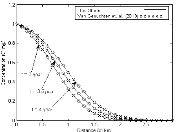
For the validation purpose, Van Genuchten et. al. (2013) obtained analytical solution for the case B1 considered as follows:
2 2
x
C C C
D u C
t x x
(20)
0
( , )t ( )
C x t f x (21)
0
0 ( )
x x
x
C
uC D ug t
x
(22)
0
x C
x
(23)
The analytical solution obtained with the conditionsf x( ) ci 0, 0 and g t( )c0 is as follows:
0
( , ) exp
2 2 x x 2 x
c x ut ux x ut C x t erfc erfc
D
tD tD
(24)
This is an identical solution when we put k1 0 k2 in Eq. (19).
Fig. 6. The comparison of pollutant concentration profile along the flow direction (x) (this study and Van Genuchten et. al. (2013)) at three different times.
Fig.6 plots the curves showing concentration between this study and Van Genuchten et. al. (2013) in the aquifer at t = 3, 3.5 and 4 years with constant dispersion and velocity along the flow direction. From this Fig. it is quite clear that the rate of decrease of pollutant concentration is faster for the small time
period as compare to the long time periods as shown in the Fig.6. The pollutant concentration decreases when distance increases and towards the exit boundary.
0 t 0.25 years for the particular distance x = 0.5 km and 0 t 0.45 years for the particular distance x = 0.75 km but after that times the pollutant concentration rapidly increases sharply with increasing
time. Overall, it is observed that the rate of increase of pollutant concentration is faster for the particular distance x = 0.25 km as compare to the long particular distances which is shown in Fig. 7.
Fig. 7. The comparison of pollutant concentration profile with increasing time (this study and Van Genuchten et. al. (2013)) at three fixed location of the model domain.
CONCLUSIONS
An analytical solution of 1-D ADE with time dependent dispersion and velocity coefficients in an aquifer of semi-infinite with an additional source-sink term is derived. The solution is illustrated with assumed values of dispersion coefficient and velocities. The following points of the conclusion are drawn from the solution and graphical representation:
1. Laplace transform is used to obtain the closed form analytical solution of the ADE.
2. The source-sink term incorporated in the system exhibits its effect after the concentration reaches the peak. Then, concentration decreases with distance rapidly and asymptotically tends to zero. This rapidly decreasing effect with distance is visible only for the additional sink term incorporated in the system.
3. The groundwater pollutant
concentration increasing with respect to time means that pollutant concentration
after some time increases for the value of dispersion and velocity. Since the additional function is a strictly increasing function with time, the graph is realistic with time. Also, the pollutant concentration is increasing with respect to aquifer distance but after some distance the peak contaminant concentration decreases as distance increases and asymptotically approaches zero for the remedial measure, namely, sink term.
4. The contaminant concentration profile is sensitive to dispersion and velocity coefficients, as for a small change in dispersion and velocity coefficient an abrupt change in the contaminant concentration profile is observed.
dispersion and velocity. But for the small particular distance the rate of increase of pollutant concentration is faster and sharply as compare to the other particular distances.
NOMENCLATURE Symbols Description
x Groundwater flow direction [L]
t Time [T]
C (x,t) Pollutant concentration in the liquid phase [ML-3]
D Dispersion coefficient [L2T -1]
u Seepage velocity coefficient [LT -1]
C0 Initial solute concentration [ML-3] 1
0
c
Concentration rate of fluid source [ML-3 T -1]D0 Initial dispersion coefficient [L2 T -1]
u0
Initial seepage velocity coefficient [LT -1]
k1, k2 Flow resistance coefficient [T -1]
a0, b0 Constant coefficients [L] ACKNOWLEDGMENT
The authors are thankful to the Indian Institute of Technology (Indian School of Mines), Dhanbad, India, for providing financial support for Ph.D. studies under the UGC-JRF scheme. This work is partially supported by the DST (SERB) Project EMR/2016/001628. The authors are thankful to the editor and reviewers for their constructive comments, which helped improve the quality of the paper.
GRANT SUPPORT DETAILS
The present research has been financially supported by Indian Institute of Technology (Indian School of Mines), Dhanbad, India, for Ph.D. studies under the University Grant Commission, New Delhi-JRF scheme. (Grant No.: June2014, 415611).
CONFLICT OF INTEREST
The authors declare that there is not any conflict of interests regarding the publication of this manuscript. In addition, the ethical issues, including plagiarism, informed consent, misconduct, data fabrication and/ or falsification, double publication and/or submission, and redundancy has been completely observed by the authors.
LIFE SCIENCE REPORTING
No life science threat was practiced in this research.
REFERENCES
Akbarpour, S., and Niksokhan, M.H. (2018). Investigating effects of climate change, urbanization, and sea level changes on groundwater resources in a coastal aquifer: an integrated assessment. Environ. Monit. Assess., 190(10); 579. Amin, M.M., Veith, T.L., Collick, A.S., Karsten, H.D. and Buda, A.R. (2017). Simulating hydrological and nonpoint source pollution processes in a karst watershed: A variable source area hydrology model evaluation. Agric. Water Management, 180; 212-223.
Aral, M.M. and Liao, B. (1996). Analytical solutions for two-dimensional transport equation with time-dependent dispersion coefficients. J. Hydrol. Eng., 1(1); 20-32.
Bai, B., Li, H., Xu, T. and Chen, X. (2015). Analytical solutions for contaminant transport in a semi-infinite porous medium using the source function method. Comput. Geotech., 69; 114-123. Balla, K., Kéri, G., and Rapcsák, T. (2002). Pollution of underground water: a computational case study using a transport model. J. Hydroinform., 4(4); 255-263.
Bauer, M., Fulda, B., and Blodau, C. (2008). Groundwater derived arsenic in high carbonate wetland soils: Sources, sinks, and mobility. Sci. Total Environ., 401(1); 109-120.
Chatterjee, A. and Singh, M.K (2018). Two-dimensional advection-dispersion equation with depth-dependent variable source concentration. Pollut., 4(1); 1-8.
Chen, J.S. and Liu, C.W. (2011). Generalized analytical solution for advection-dispersion equation in finite spatial domain with arbitrary time-dependent inlet boundary condition. Hydrol. Earth Syst. Sci., 15(8); 2471-2479.
De Smedt, F., Brevis, W. and Debels, P. (2005). Analytical solution for solute transport resulting from instantaneous injection in streams with transient storage. J. Hydrol., 315(1); 25-39.
Freeze, R.A. and Cherry, J.A. (1979). Groundwater Prentice-Hall International. New Jersey: Englewood Cliffs.
Jia, X., Zeng, F. and Gu, Y. (2013). Semi-analytical solutions to one-dimensional advection–diffusion equations with variable diffusion coefficient and variable flow velocity. App. Math. Comput., 221; 268-281.
Kral, U., Brunner, P.H., Chen, P.C. and Chen, S.R. (2014). Sinks as limited resources? A new indicator for evaluating anthropogenic material flows. Ecol. Indic., 46; 596-609.
Leij, F.J., Priesack, E. and Schaap, M.G. (2000). Solute transport modeled with Green's functions with application to persistent solute sources. J. Contam. Hydrol., 41(1); 155-173.
Logan, J.D. and Zlotnik, V. (1995). The convection-diffusion equation with periodic boundary conditions. App. Math. Letters, 8(3); 55-61.
Moutsopoulos, K.N., Poultsidis, V.G., Papaspyros, J.N. and Tsihrintzis, V.A. (2011). Simulation of hydrodynamics and nitrogen transformation processes in HSF constructed wetlands and porous media using the advection–dispersion-reaction equation with linear sink-source terms. Ecol. Eng., 37(9); 1407-1415. Natarajan, N. and Kumar, G.S. (2017). Spatial moment analysis of multispecies contaminant transport in porous media. Environ. Eng. Res., 23(1); 76-83.
Nemitz, E., Sutton, M.A., Gut, A., San José, R., Husted, S. and Schjoerring, J.K. (2000). Sources and sinks of ammonia within an oilseed rape canopy. Agric. For. Meteorol., 105(4); 385-404. Sander, G.C. and Braddock, R.D. (2005). Analytical solutions to the transient, unsaturated transport of water and contaminants through horizontal porous media. Adv. Water Resour., 28(10); 1102-1111. Shi, X., Lei, T., Yan, Y. and Zhang, F. (2016). Determination and impact factor analysis of hydrodynamic dispersion coefficient within a gravel layer using an electrolyte tracer method. Int. Soil and Water Conser. Res., 4(2); 87-92.
Singh, M.K. and Kumari, P. (2014). Contaminant concentration prediction along unsteady groundwater flow. Modelling and Simulation of Diffusive Processes, Series: Simulation Foundations, Methods and Applications. Springer. XII. 257-276.
Singh, M. K., Singh, V. P. and Das, P. (2015). Mathematical modeling for solute transport in aquifer. J. Hydroinform., 18(3), 481-499.
Srinivasan, V. and Clement, T.P. (2008). Analytical solutions for sequentially coupled one-dimensional
reactive transport problems–Part I: Mathematical derivations. Adv. Water Resour., 31(2); 203-218. Thakur, C.K., Chaudhary, M., van der Zee, S.E.A.T.M. and Singh, M.K. (2019). Two dimensional solute transport with exponential initial concentration distribution and varying flow velocity. Pollut., 5(4); 721-737.
Tkalich, P. (2006). Derivation of high-order advection-diffusion schemes. J. Hydroinform., 8(3); 149-164.
Van Genuchten, M.T. (1981). Analytical solutions for chemical transport with simultaneous adsorption, zero-order production and first-order decay. J. Hydrol., 49(3-4); 213-233.
Van Genuchten, M.T., Leij, F.J., Skaggs, T.H., Toride, N., Bradford, S.A. and Pontedeiro, E.M. (2013). Exact analytical solutions for contaminant transport in rivers 1. The equilibrium advection-dispersion equation. J. Hydrol. Hydromech., 61(2); 146-160.
Van Hecke, M., Storm, C. and van Saarloos, W. (1999). Sources, sinks and wavenumber selection in coupled CGL equations and experimental implications for counter-propagating wave systems. Physica D: Nonlinear Phenomena. 134(1); 1-47.
van Kooten, J.J. (1994). Groundwater contaminant transport including adsorption and first order decay. Stochastic Hydrol. and Hydraul., 8(3); 185-205.
Wang, J., Shao, M.A., Huang, L. and Jia, X. (2017). A general polynomial solution to convection– dispersion equation using boundary layer theory. J. Earth Syst. Sci., 126(3); 40.
West, M.R., Kueper, B.H. and Novakowski, K.S. (2004). Semi-analytical solutions for solute transport in fractured porous media using a strip source of finite width. Adv. Water Resour., 27(11); 1045-1059.
You, K. and Zhan, H. (2013). New solutions for solute transport in a finite column with distance-dependent dispersivities and time-distance-dependent solute sources. J. Hydrol., 487; 87-97.