The IUFP Algorithm for Generating Simulation Heart
Elham Shadkam
iand Abdollah Aghaie
iiReceived 04 Dec 2011; received in revised 08 May 2012; accepted 09 Dec 2012
ABSTRACT
In all systems simulation, random variates are considered as a main factor and based of simulation heart.
Actually, randomization is inducted by random variates in the simulation. Due to the importance of such a
problem, a new method for generation of random variates from continuous distributions is presented in this
paper. The proposed algorithm, called uniform fractional part (UFP) is simpler and more efficient compared
with other methods of random variates generation. Despite useful consequences, this algorithm has several
shortcomings such as 1) being approximate, 2) not accessibility of the inverse of cumulative density
function (CDF) for all distributions in order to determine the cut-off points and 3) truncating the tails of
infinite distributions, which all of the aforementioned shortcomings reduce the precision and speed of the
algorithm. The main goal of this research is proposing the improved version of this algorithm (IUFP)
through recognizing its deficiencies.
KEYWORDS
Random Variates generation, Simulation, Uniform Fractional Part (UFP)
i* Corresponding Author, E. Shadkam, PhD student, Department of Industrial Engineering, Isfahan University of Technology, Isfahan, Iran
ii A. Aghaie, Professor, Department of Industrial Engineering, K.N. Toosi University of Technology, Tehran, Iran ([email protected])
1. INTRODUCTION
Random variates are considered as the main factors in all systems simulation in as much as they are known as simulation heart. Most of computer languages have functions or sub-programs to generate random variates and similarly, simulation languages also employ the algorithms of random variates generation to derive time events and other random variables. By developing simulation and computer utilization, more attention is paid to various methods of random variates generation [1]. All of the books associated with discrete event simulation or Mont Carlo’s methods have at least one chapter concerning this field which shows the importance of this problem. Generation of random variates is one of the common research areas in statistics, operations research and computer science [2]. The random variates generation was paid attention as a research area when the feasibility of Mont Carlo’s tests was studied in the Second World War [3]. These are different Application of this area. As an instance, in Mont Carlo’s methods, to solve the various problems such as random optimization, Mont Carlo’s integration, solution of the linear equations and etc is applicable.
Random variates play a key role in the implementations of simulation techniques. During the past few years, there has been an increasing interest in developing new techniques based on random variates [4].
The generation of non-uniform random deviates has come a long way, from methods dating back to a time prior to the era of the computer to the latest novel methods, such as the Ziggurat and vertical strip. While some methods are general in nature, some others are intended for a particular distribution. Among the algorithms developed so far, some are widely used and/or are more efficient than others. The main classifications for these algorithms are:
1.The Inverse Transform methods 2. The Composition methods 3.The Acceptance Rejection methods
Among the presented algorithms, some of them are more useful and efficient than the others. The best one is presented by Izady and Mahlooji in 2005. This algorithm is simple, precise, efficient and quick. One may refer to [5] to see its superiority.
correlated deviates and being applicable to all density functions, regardless of their parameter values.
In spite of useful consequences, this algorithm has some shortcomings. In this paper, an improved version of this algorithm is proposed by corrective approaches through recognizing its deficiencies. By implementation of the proposed approaches, the outcomes of the improved algorithm are then compared with the original algorithm. As will be demonstrated in the next sections, our algorithm outperforms the original one. Since universal algorithms are applicable to all continuous distributions and the proposed algorithm has such a property, it will be applied on the normal and exponential distributions [6].
The main requirement component of all methods of random variates generation is existence of a random numbers generator, which is assumed such a generator is available. By random numbers, the author means generated uniform random variates on [0, 1] [7].
The rest of the paper is organized as follows. In Section 2, the UFP algorithm will be explained. Section 3 states the shortcomings of the original UFP algorithm in which the corrective approaches for 1) approximate form of the algorithm, 2) determining of cut-off points and 3) generating random variates from tails of unlimited distributions are fully presented. In Section 4 the improved UFP called IUFP is developed and Section 5 described how to implement the IUFP algorithm on various distributions, such as normal and exponential ones. Finally, Section 6 provides of conclusions and future work.
2. DESCRIPTION OF THE UNIFORM FRACTIONAL PART
(UFP) ALGORITHM
This algorithm is one of the latest presented methods proposed by Izady and Mahlooji. It is an approximate algorithm which is mainly used for continuous distributions and is appropriate for simulation of models which no change is made on distribution parameters during the simulation process, due to its short marginal time and large setup time.
Of other advantages of this algorithm is the need of only one random number for generating a random variate in the optimized status. The required calculations for random variate generation are linear. The volume of programming is little and the body of the algorithm is the same for all distributions. The only dissimilar step for the various distributions is the setup stage of the algorithm in which the cut-off points are determined based on the inverse of the desired cumulative distribution function (CDF). The algorithm is based on a theorem given in [8], page 72 and restated below.
Theorem 1: [8] Fractional part of sum of two independent random variables with uniform distribution on [0, 1], itself has uniform distribution on [0, 1].
In other words, if x and R1 are two independent random variates on U[0, 1] and R2 is defined as
R x
x R
R2 1 1 , then the variable R2 has a uniform distribution. The
denotes the biggest integer number less than or equal to . By generalizing this theorem, one can say that if x has any desired continuous distribution, random variable R2 has uniform distribution on [0,1]. Consequently, continuous random variable x can be generated using the above equation (namely by means of two random numbers such as R1 and R2). According to [9], the above equation then can be rewritten as:(1)
R x
R R
x 2 1 1
In fact, the UFP algorithm is summarized as:
1) Generate R1and R2 as two independent uniform random numbers.
2) Generate a value for
xIf R2R1then xR2R1
x ; otherwise,
12
1
R R x x
Figure 1: Probabilities concerning
x [5].Initially, an integer value in range of x is randomly selected (one of the separated columns in Fig. 1) and a value of R2−R1 is then added to such a random selected integer to make a random variate, where R1 and R2 are two independent uniform random variables on [0,1].
Some applications of the UFP algorithm are:
1.Generation of continuous random variates from the desired continuous distributions such as gamma, beta, normal and etc.
2.Generation of the correlated random variates [5]. 3.Generation of the random variates associated with ordering statistics [10].
4.Generation of random numbers [11].
arbitrary cut-off points, 3) equal area approach, 4) different approaches to determine the tails of the distribution, 5) reduction approach for the number of used random numbers, when d = 1, 6) reduction approach for the number of used random numbers with arbitrary values of d, 7) recycling uniform random number approach when d = 1, 8) recycling uniform random number approach with arbitrary values of d and finally 9) speeding up to generate Int (x). By Int (x), the author means the integer number of x.
It is noticeable that the main method (in this paper) is the latest aforementioned algorithm (Algorithm 9 in above) and our focus in this paper is on this algorithm. First of all, we survey the deficiencies of this algorithm and improvement approaches are then adapted to this algorithm. So, of presented algorithms in the UFP evolution, only the associated steps with algorithm 9 are
presented here as follows (called algorithm A in this paper):
1) Set uniform probability p and then generate the cut-off points a1, a2,..., anas well as di= ai+1− ai for i= 1, 2, ..., n−1.
2) Generate a random number u.
3) Determine the index i by calculating the value of
1
p u
and then identify a value for ai, i.e., Int(x) based on the value of i.
4) Generate a random number u’ . 5) Find x as x = ai+ u’ di
3. SHORTCOMINGS OF THE ORIGINAL UFP ALGORITHM Despite a large number of advantages, the UFP algorithm has several shortcomings listed in Table 1. TABLE 1
SHORTCOMINGS OF UFP ORIGINAL ALGORITHM
Expected results than algorithm A Algorithm
name Corrective approach
Shortcoming of the algorithm No.
Higher precision B
Using uniform hat and squeeze functions
Approximate form of the algorithm 1
Simplicity of the algorithm C&D
Using hat or squeeze function and estimate the area approximately Not accessibility to inverse CDF for
all distributions in order to determine the cut-off points
2
Higher precision E
Using hybrid approach Truncating the tails of infinite
distributions 3
A. Corrective approach for approximate form of the algorithm
Since the main method (Algorithm 9 called A method) is an approximate algorithm, it can be transformed to a near exact method by defining a hat function h(x) and using the acceptance-rejection logic [12],[13].
If for a random pair (x, y), in which x are generated from any method and y from a hat function, respectively, the inequality y ≤ f(x) is satisfied, the generated points are then scattered uniformly under the density function f(x) and consequently the points have f(x) distribution, since y values are uniformly under the density function f(x). This is the main purpose of using the hat function. Since the evaluation of the acceptance condition, i.e, y ≤ f(x) is a time consuming step for most of distributions, we can accelerate the algorithm by manipulating the squeeze function (S(x)). For example the lower bound of S(x) can be found in such a way that the inequality s(x) ≤ f(x) is satisfied. In this case, if (x, vh(x)) pair values (in which v is a random number and h(x) is the hat function) are under S(x), the random variate x could be accepted with no evaluation of the density function [14]. In fact, in algorithm B, local or piecewise hat and squeeze functions are employed. It is noticeable that the determination of hat
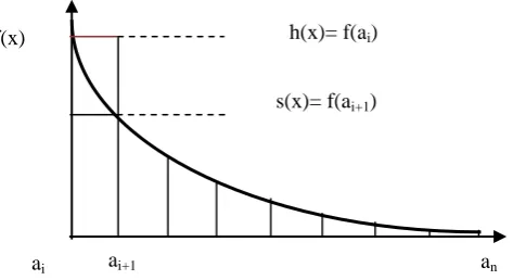
and squeeze functions depends on the form of the function. If the given function is descending (such as Fig. 2), hat and squeeze functions are considered uniformly on [0, f(ai)] and [0, f(ai+1)] for each interval, respectively, but
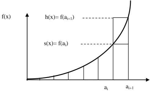
if the foresaid function is ascending, (Fig. 3), hat and squeeze functions are defined uniformly on [0, f(ai+1)] and
[0, f(ai)] intervals, respectively [15].
Figure 2: Hat and squeeze functions for descending given functions.
f(x) h(x)= f(ai)
s(x)= f(ai+1)
Figure 3: Hat and squeeze functions for ascending functions.
In this approach, the hat function defined for x is located in the interval (ai, ai+1) which is uniformly defined on [0,f(ai)] and also squeeze function uniformly on [0,f(ai+1)].
Steps of algorithm B (UFP algorithm with hat and squeeze functions) are as follows:
1) Generate x with algorithm A. 2) Generate a random number v. 3) Calculate the value of y = v f (ai ).
4) If y ≤ s(x) = f (ai+1), then, go to step (6) (the evaluation step for the squeeze function), otherwise; go to step (5)
5) If y ≤ f(x), then, go to step (6) (the evaluation step for f(x) function), otherwise; go to step (1).
6) return x.
If the given distribution function has a more complicated form, define hi and si as:
(2)
( ): 1
sup
i i
i f x a x a
h
(3)
( ): 1
inf
i i
i f x a x a
s
Inf and sup stand for infimum and supremum respectively. They are typically used on sets of real numbers. The infimum or the greatest lower bound of a set S is the lowest number of set S, Similarly, the supremum is the least upper bound of the set, or the largest number.
Therefore, hat and squeeze functions are generated uniformly on [0, hi] and [0, si], respectively. Since we
ignore many conditions by determining si and hi, the performance of the proposed method will be increased, which is notable as opposed to the large setup time. A.1. Validation of the corrective approach for the approximate form of the algorithm
In order to validate the proposed approaches, the improved algorithms obtained from these approaches (algorithm B) are compared to the original one. The exponential distribution has been used to do so. Of course, the algorithm B is applicable for all other continuous distributions. As pointed out earlier, the proposed
algorithm is a universal one and has no limitation of usage for any special distribution.
In order to validate, two criteria, i.e., speed and precision are employed in this research [16].
The main factors in the study of algorithms are: simplicity, speed, robustness and coverage, the number of used random numbers, and memory requirements. The most important parameters in the study of algorithms are speed and accuracy.
In this way, one million data have been generated to evaluate the speed criterion. The generation speed of a random variate has been calculated in micro seconds (µs). Also, the P-value parameter in Anderson-Darling test in 95% confidence level is used for the precision criterion.
The Anderson–Darling test is a statistical test of whether a given sample of data is drawn from a given probability distribution. The Anderson-Darling statistic Measures how well the data follow a particular distribution. The better the distribution fits the data, the smaller is this statistic. This given below:
))] 1 ( 1 ln( ) ( [ln 1(2 1) 1
2
n F xi F xn i
i i
n n A
The hypotheses for the Anderson-Darling test are: H0: The data follow a specified distribution
H1: The data does not follow a specified distribution
It is worth mentioning that the algorithms have been performed with Borland compiler of C++ 5.02 under 32-Bit platform and evaluation parameters have been calculated using Minitab 14.0 software. Generating time can greatly reduce via more professional coding. An example of generation time of random variates for beta distribution with other methods is presented in Table 2 with a more advanced coding program. Since our objective is comparison between the original and improved version of the UFP method, the coding has been simplified in this paper.
TABLE 2
COMPARISON BETWEEN UFP AND THE OTHER ONE FOR SPEED CRITERION (IZADY,2005)
Speed (µs) Algorithm
0.25 UFP
1.3 TDR
2.3 BPRB
1.85 BPRS
2.1 B4PE
2.7 Sakasegawa
3.3 Cheng
1.5 Strip
1.4 NI
6.62 Johnk
Table 3 shows the comparison results of various criteria for algorithms on exponential distribution with different parameters. In the following table, AD means the value of the Anderson-Darling statistics test and R is the average number of rejected values of 1000 generated ai ai+1
f(x) h(x)= f(ai+1)
random values. Finally, f means the number of times the density function is evaluated for generation of 1000 random variates. Number of cut-off points in Table 3 is equal to 128 sections, which are considered as power of two. We employ power of two owing to the capability of the programming in such a policy.
As could be seen in Table 3, a foresaid methods are robust and stable with respect to changes of distribution parameters, i.e., different β. Algorithm B yields higher P-values and lower Anderson-Darling coefficient than algorithm A, therefore, algorithm B is more precise than A.
The dissimilarities between the numbers of Tables 2 and 3 for the speed of the UFP algorithm are due to the different coding and run environment.
The results demonstrate that by increasing the number of cut-off points, the values of f and R decrease and consequently, the precision of the algorithm will increase. Therefore, whatever the value of these two parameters, i.e., f and R become low, the quality of outputs will increase. Increase in the number of divisions results in decreasing the value of p and consequently increasing the algorithm precision. Hens, if p goesto zero, the precision of algorithm B approaches to the other exact methods precision, such as inverse transformation method.
TABLE 3
COMPARISON OF ALGORITHMS FOR APPROXIMATE FORM
Β Algorithm p=1/128
n=128 Spee
d (μs) P-value
AD R F
2 A 28 0 1.494 0.182 27
B 28 15 0.373 >0.25 25
1 A 28 0 1.494 0.182 27
B 28 15 0.373 >0.25 25
0.5 A 28 0 1.494 0.182 27
B 28 15 0.373 >0.25 25
0.25 A 28 0 1.494 0.182 27
B 28 15 0.373 >0.25 25
0.1 A 28 0 1.494 0.182 27
B 28 15 0.373 >0.25 25
B. Corrective approach for determining the cut-off points
The most important step in implementing the UFP algorithm is concerned with the determination of cut-off points of a1, a2,..., an which is defined arbitrary on the x range. One of the main shortcomings of the original method is how to calculate pi which is used in
determination of the cut-off points. The method in the UFP algorithm used for the calculation of pi decreases the
speed of the algorithm and requires the inverse of CDF for each sub-interval. This matter is often difficult and unfeasible for some distribution such as normal distribution. The method used for the UFP algorithm (considering the equal area approach) acts as:
) ( ), ) ( ( , ) ( )
(a1 F a0 pa1 F 1 F a0 p a1 F 1 p
F
) 2 ( ) ) ( ( , ) ( )
(a2 F a1 p a2 F 1 F a1 p F 1 p
F
(4) ) ( 1 np F
an
As could be seen, in this approach CDF of the desired distribution is not only required, but also the inverse of CDF is needed whiles these calculations are very difficult for some distributions such as normal, gamma and etc. To solve such difficulty, the proposed approach is to use the approximate area of hat or squeeze functions instead of the precise area through the inverse of CDF. Calculations of this approach are as follows:
) 0 ( , ) )( ( , ) ( )
( 1 0 0 1 0 1
f p a p a a a f p a F a
F
1 1 2 2 1 1 2 1 ) ( , ) ) 0 ( )( ( , ) )( ( a a f p a p f p a a f p a a a
f
(5) 1 1) ( n n n a a f p a
In this approach, as could be seen, distributions CDF are not needed and the cut-off points can be determined only using the probability density function. In fact, the cut-off points can be determined through the hat or squeeze functions, instead of calculating
1 ) ( n n a a
n f xdx
p using a
simple linear equation instead of an integration equation. In algorithm C, the cut-off points are determined by means of the hat function as follows in which except the following step (first step), the rest of the algorithm is similar to the algorithm B.
1) Determine the cut-off points via equation 1 1 1 ) ( i i i i a a f p
a , (a1= 0)
Also, algorithm D uses the squeeze function to determine the cut-off points like the algorithm C, except the following step (first step), the rest of the algorithm is similar to algorithm B.
1) Determine the cut-off points by means of equation ) ( 1 1 1 i i i i a f p a a
Indeed, as pointed out earlier, the cut-off points in algorithm C are determined from the hat function but starting from the beginning of the range, unlike algorithm D, in which cut-off points are determined from the squeeze function starting from the end of the range. Figs. 4 to 6 show cut-off points and the specified areas of pi in
Figure 4: Method of determination of areas in algorithm A.
Figure 5: Method of determination of areas in algorithm C.
Figure 6: Method of determination of areas in algorithm D.
To determine the cut-off points, other approaches can be employed such as equal intervals using
i n
a a a
ai 0( n 0) . Equal intervals approach as algorithm J will be evaluated below.
B. 1. Validation of corrective approach for determining the cut-off points
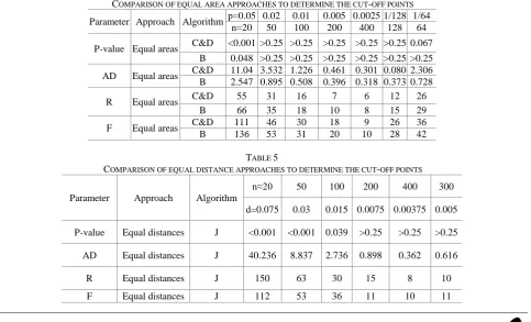
Tables 4 and 5 show the obtained results of the equal area and the equal distance approaches. . The exponential distribution has been used to do so. The approximate equal area approach (algorithm C & D) yields undesired results with lower number of divisions, whiles by increasing this divisions, the results will be improved, so that in n=128, the results of approximate area are much better than the exact area algorithm. Although the consequences of using equal distance approach (algorithm J) is to some extent desired, though equal area approach is preferred to use, since the calculation of
x is eliminated in this approach. Moreover, no explorer algorithms are needed to detect the interval which x is generated from.According to the aforementioned explanations, the approximate equal area obtained from hat function with a large number of divisions is the best approach (algorithm C & D).
TABLE 4
COMPARISON OF EQUAL AREA APPROACHES TO DETERMINE THE CUT-OFF POINTS 1/64 1/128 0.0025 0.005 0.01 0.02 p=0.05 Algorithm Approach
Parameter
64 128 400 200 100 50 n=20
0.067 >0.25 >0.25 >0.25 >0.25 >0.25 <0.001 C&D
Equal areas P-value
>0.25 >0.25 >0.25 >0.25 >0.25 >0.25 0.048 B
2.306 0.080 0.301 0.461 1.226 3.532 11.04 C&D
Equal areas AD
0.728 0.373 0.318 0.396 0.508 0.895 2.547 B
26 12 6 7 16 31 55 C&D Equal areas R
29 15 8 10 18 35 66 B
36 26 9 18 30 46 111 C&D Equal areas F
42 28 10 20 31 53 136 B
TABLE 5
COMPARISON OF EQUAL DISTANCE APPROACHES TO DETERMINE THE CUT-OFF POINTS
300 400 200
100 50
n≈20 Algorithm Approach
Parameter
0.005 0.00375 0.0075
0.015 0.03
d=0.075
>0.25 >0.25 >0.25
0.039 <0.001 <0.001
J Equal distances P-value
0.616 0.362 0.898
2.736 8.837 40.236 J
Equal distances AD
10 8
15 30 63 150 J
Equal distances R
11 10 11
36 53 112 J
Equal distances F
pi
pi
C. Corrective approach to generate random variates from unlimited tails distributions
Another main problem of the UFP algorithm is truncating the tails of distribution which extremely decreases algorithm precision. Hybrid algorithms can be applied to solve such a difficulty. To do so, initially the UFP algorithm is employed for body of distribution and an acceptance-rejection method with an exponential hat function will be then applied for the tails of distribution. Such an algorithm can be stated in terms of the following algorithm, i.e., algorithm E which is a hybrid approach for the tails of distribution as follows:
1) Select an interval randomly (i),
2) If i ≠ n, follow the UFP algorithm, otherwise follow the below algorithm:
2-1)Generate random numbers u and v 2-2)Calculate the value of x 1ln(u)
(inverse
transformation method is used to generate the random variates from the exponential hat function),
2-3)Compute the value of yv
ex.2-4)If y f(x) then go to step (3), otherwise; go to step (1).
3) Return x.
The above algorithm is a general one which can be
used for tails of all distributions, however if a higher precision is aimed, more specialized algorithms for tails of various distributions should be employed [17]. The CDF of truncated hat function can be calculated as follows:
, . 0 ) ( ) ( ) ( ) ( ) ( w o b x ifa u a F b F a F x F x F
) (x F e e e e b a x a
Therefore, the value of x is calculated based on Eq.6 .
)) 1 ( ln( 1 1 u e
x an
(6)C.1. Validation of corrective the approach for the distribution tails
As could be seen, the results of the algorithm E have been considerably improved as compared to the algorithm B without decreasing the algorithm speed. For this, the exponential distribution has been used. It is worth mentioning that the last row of Table 6 shows the number of generated values of distribution tails which are neglected in the UFP algorithm.
TABLE 6
COMPARISON OF ALGORITHMS FOR TAILS OF DISTRIBUTIONS
1/64 1/128 0.0025 0.005 0.01 0.02 p=0.05 Algorithm Parameter 64 128 400 200 100 50 n=20 >0.25 >0.25 >0.25 >0.25 >0.25 >0.25 0.048 B P-value 0.12 >0.25 >0.25 >0.25 >0.25 >0.25 0.115 E 0.728 0.373 0.318 0.396 0.508 0.895 2.547 B AD 1.801 0.318 0.261 0.379 0.221 1.084 1.834 E 29 15 8 10 18 35 66 B R 38 20 8 13 26 43 59 E 42 28 10 20 31 53 136 B f 41 21 10 14 16 48 67 E 25 25 28 28 28 28 28 B Speed (μs) 25 25 28 28 28 28 28 E 0 0 0 0 0 0 0 B Tail 15 8 5 8 12 22 69 E
4. THE IMPROVED UFP(IUFP)
All the proposed approaches are employed together in the final algorithm. In the improved version of UFP, called IUFP, the squeeze and the hat functions are employed, the determination method of cut-off points is changed and hybrid approach is applied for the tails of unlimited distributions. The IUFP algorithm is
implemented on normal and exponential distributions in this paper although it is applicable for all continuous distributions.
The general definition of squeeze and hat functions (Eqs. 7 and 8) are used for the IUFP algorithm.
(7)
( ):
min
( ), ( )
inf 1 1
i i i i
i f a a x a f a f a
s
(8)
( ):
max
( ), ( )
sup 1 1
i i i i
i f a a x a f a f a
1) Determine the cut-off points based on the approximate equal area approach (algorithm C & D) using
1 1 1
)
(
i
i i
i a
a f
p a
2) Specify the squeeze and the hat functions from Eqs. 7 and 8
3) Select one of random the interval based on the equal area approach using
1
p u i
4) If i ≠ n:
4-1) Return ai-1 from the selected interval as Int(x)
4-2) Generate random numbers u and v 4-3) Calculate xai1udi
4-4) Compute the value of y base on vh(i)
4-5) If ys(i), go to step 7), otherwise; go to (4-6)
4-6) If y f(x), go to step (4-7), otherwise; go to step (3)
4-7) Return x 5) If i = n:
5-1) Generate random numbers u and v 5-2) Calculate the value of x 1ln(u)
5-4) Calculate the value of y based on
) exp( x v
5-5) If y f(x) then return x, otherwise; go to step (3)
This algorithm is applicable for all continuous distributions, although we can use the limited definition for hat and squeeze functions (Eqs. 9 and 10). In the latter case, the algorithm is only applicable for the distributions of normal, exponential, gamma (α≤1), weibull (α≤1) and beta (α≤1), as well as all descending distributions.
(9)
( ):
( )inf 1 1
i i i
i f a a x a f a
s
(10)
( ):
( )sup i i 1 i
i f a a x a f a
h
5. IMPLEMENTATION OF IUFP ON VARIOUS
DISTRIBUTIONS
The results of applying the IUFP algorithm on normal and exponential distributions are summarized as follows: by means of random variates generation via the algorithm, the outputs will be tested by the Anderson-Darling test for fitness evaluation to the desired distribution. The corresponding plots are also presented in the following sub-section.
A. Normal distribution
Due to the key role of normal distribution in statistical applications, it is necessary to develop efficient and reliable methods for the random variate generation of this
distribution. To generate the random variates of normal distribution with parameters (μ,σ), firstly, standard normal variates should be generated and then replace the obtained values in xσ+μ. In this distribution, an extra random number is used to determine the sign of the random variate.
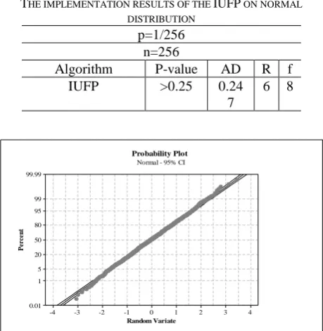
TABLE 7
THE IMPLEMENTATION RESULTS OF THE IUFP ON NORMAL DISTRIBUTION
p=1/256 n=256
f R AD P-value Algorithm
8 6 0.24
7 >0.25 IUFP
4 3 2 1 0 -1 -2 -3 -4 99.99
99
95
80
50
20
5
1
0.01
Random Variate
P
er
ce
n
t
Normal - 95% CI Probability Plot
Figure 7: Probability plot for normal distribution.
One thousand normal random variates are generated using the IUFP algorithm. The following parameters are averagely obtained considering the number of evaluations of objective function and the number of algorithm iterations:
006 . 1 ) ( , 0008 . 0 )
(#f E I
E
.According to the obtained parameters, it could be seen that applying this algorithm on normal distribution is very practical, since generation of a random variate needs 1.006 iterations of algorithm and 0.008 times to evaluate the density function, which is very desired.
B. Exponential distribution
Similar to the normal distribution, all the aforementioned steps are applied to the exponential distribution. The results of implementation of the IUFP algorithm on exponential distribution are shown in the Table 8.
TABLE 8
THE IMPLEMENTATION RESULTS OF THE IUFP ON EXPONENTIAL DISTRIBUTION
p=1/128 n=128
F R AD P-value
Β
Algorithm
21 20 0.237 >0.25
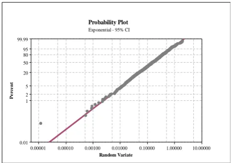
Figure 8: Probability plot for exponential distribution.
Similar to the previous section, 1000 random variates are generated and the following parameters are averagely obtained using the evaluation number of objective function as well as the numbers of algorithm iterations:
02 . 1 ) ( , 021 . 0 )
(#f E I
E
As could be seen, we need only one iteration of algorithm as well as a few number of density function evaluations to generate a random variate. According to the obtained results, the IUFP algorithm is very practical for
exponential distribution.
6. CONCLUSIONS AND FUTURE WORK
In this study, we presented the universal UFP algorithm to use for various distributions which are more efficient than the other algorithms in this context. Although the UFP algorithm has useful results, it has several shortcomings. In this paper, we tried to eliminate such shortcomings using the improved version of this algorithm (IUFP) through recognizing its deficiencies. The IUFP algorithm showed better results in comparison with the UFP algorithm. According to the results, IUFP algorithm almost covers all characteristics of an ideal random variate generation algorithm.
As a direction for future research, it would be interesting to study two various areas. The one is associated with further improvement of the algorithm, such as determining the cut-off points via other approaches or using the specialized algorithm for non-truncating tails of unlimited distributions, and the second one could be finding new applications for such an algorithm, such as random variate generation from discrete distributions.
7. REFERENCES
[1] Banks, J.; Handbook of simulation principle, methodology, advances, applications and practice, 3nd Edition, New York: John Wiley & Sons, 1998.
[2] Hung, Y. C.; Balakrishnan, N.; Cheng C. W.; “Evaluation of algorithms for generating Dirichlet random vectors”, Journal of Statistical Computation and Simulation, 2010.
[3] Banks, J.; Carson, J.S.; Nelson, B.L.; Nicol, D.M.; Discrete-event system simulation, 1nd Edition, Upper Saddle River: Pear-son Prentice Hall, 2005.
[4] Ormann, W.; Erflinger, G.; “The transformed rejection method for generating random variables, an alternative to the ratio of uniforms method” Communications in Statistics - Simulation and Computation, vol. 23, 3, p.p. 847 – 860, 1994.
[5] Mahlooji, H.; Jahromi, A.E.; Mehrizi, H.A.; Izady,N.; “Uniform Fractional Part: A simple fast method for generating continuous random variates”, Scientia Iranica, vol. 15,5, p.p. 613-622, 2008. [6] Jones, M. C A.; Lunn, D.; “Transformations and random variate
generation: generalised ratio-of-uniforms methods”, Journal of Statistical Computation and Simulation, vol. 55, 1, p.p. 49-55, 1996.
[7] Cheng, R. C. H.; Feast, G. M.; “Some simple gamma variate generators”, appl statist, vol. 28,3, p.p. 290-295, 1979.
[8] Morgan, B.J.T.; Elements of simulation, 1ed Edition, London: Chapman and Hall, 1984.
[9] Mahlooji, H.; Izady, N.; “Developing a Wide Easy-to-Generate Class of Bivariate Copulas”, Communications in Statistics -Theory and Methods, vol. 37, p.p. 1919–1929, 2008.
[10] Mahlooji, H.; Mehrizi, H.A.; Farzan, A.; “A fast method for generating continuous order statics based on uniform fractional part”, Proc. 35th International Conference on Computers and Industrial Engineering, p.p. 1355-1360, 2004.
[11] Mahlooji, H.; Mehrizi, H.; Sedghi, N.; “An efficient, fast and portable random number generator”, Proc.35th International Conference on Computers and Industrial Engineering, p.p. 1361-1366, 2004.
[12] Devroye, L.; “A note on approximations in random variate generation”, Journal of Statistical Computation and Simulation, vol. 14, 2, p.p. 149-158, 1982.
[13] Devroye, L.; “Random variate generation for the digamma and trigamma distributions”, Journal of Statistical Computation and Simulation, vol. 43, 3, p.p. 197-216, 1992.
[14] Ahrens, J.H.; Dieter, U.; “Generating gamma variates by a modified rejection technique”, Communications of the ACM, vol. 25, p.p. 47-54, 1982.
[15] Hormann, W.; Leydold, J.; Derflinger,G.; Automatic nonuniform random variate generation, 1nd Edition, New York: Speringer-Verlag, 2004.
[16] Franklin, M. A.; Sen, A.; “Comparison of exact and approximate variate generation methods for the erlang distribution”, Journal of Statistical Computation and Simulation, vol. 4, 1, p.p. 1-18, 1975. [17] Laud, P.W.; Damien, P.; Shively, T. S.; “Sampling Some
Truncated Distributions Via Rejection Algorithms”, Communications in Statistics - Simulation and Computation, vol. 39, 6, p.p. 1111-1121, 2010.
10.00000 1.00000 0.10000 0.01000 0.00100 0.00010 0.00001 99.99
95 80 50
20
5
2 1
0.01
Random Variate
P
e
rc
e
n
t
Exponential - 95% CI
![Figure 1: Probabilities concerning x [5].](https://thumb-us.123doks.com/thumbv2/123dok_us/8944712.1854080/2.595.305.529.265.503/figure-probabilities-concerning-x.webp)