When Decision Meets Estimation: Theory and Applications

(1)

University of New Orleans University of New Orleans

ScholarWorks@UNO

University of New Orleans Theses and

Dissertations Dissertations and Theses

12-15-2007

When Decision Meets Estimation: Theory and Applications

Ming Yang

University of New Orleans

Follow this and additional works at: https://scholarworks.uno.edu/td

Recommended Citation Recommended Citation

Yang, Ming, "When Decision Meets Estimation: Theory and Applications" (2007). University of New Orleans Theses and Dissertations. 627.

https://scholarworks.uno.edu/td/627

(2)

When Decision Meets Estimation: Theory and Applications

A Dissertation

Submitted to the Graduate Faculty of the University of New Orleans

in partial fulfillment of the requirement for the degree of

Doctor of Philosophy in

Engineering and Applied Science

by Ming Yang

B.S., Peking University, 1997

(3)

c

(4)

Acknowledgment

This research was supported in part by ARO grant W911NF-04-1-0274, NASA/LEQSF grant (2001-4)-01, Navy through Planning Systems Contract # N68335-05-C-0382, High-Performance Networking Program of the Office of Science, U. S. Department of Energy under Contract DE-AC05-00OR22725 with UT-Battelle, LLC. and DoD DURIP program via grant W911NF-05-1-0107.

I would like to offer my deepest gratitude to my major advisor, Dr. X. Rong Li, for his continuous encouragement, timely help, and insightful suggestions during the past more than five years.

I would also thank Dr. Huimin Chen, Dr. Jing Deng, Dr. Vesselin Jilkov, and Dr. Tumulesh K.S. Solanky for serving on my thesis committee, and for their constructive and valuable comments on the dissertation. I also appreciate Dr. Stephen Lipp and Dr. Dongmin Wei for serving on my doctoral qualifying exam. Special thanks go to Dr. Chen for his long-term collaboration, advice and friendship.

(5)

(6)

Abstract

In many practical problems, both decision and estimation are involved. This dissertation intends to study the relationship between decision and estimation in these problems, so that more accurate inference methods can be developed.

Hybrid estimation is an important formulation that deals with state estimation and model structure identification simultaneously. Multiple-model (MM) methods are the most widely-used tool for hybrid estimation. A novel approach to predict the Internet end-to-end delay using MM methods is proposed. Based on preliminary analysis of the collected end-to-end delay data, we propose an off-line model set design procedure using vector quantization (VQ) and short-term time series analysis so that MM methods can be applied to predict on-line measurement data. Experimental results show that the proposed MM predictor outperforms two widely used adaptive filters in terms of prediction accuracy and robustness.

(7)

At last, a surveillance testbed is being built for such purposes as algorithm development and performance evaluation. We try to use the testbed to bridge the gap between theory and practice. In the dissertation, an overview as well as the architecture of the testbed is given and one case study is presented. The testbed is capable to serve the tasks with decision and/or estimation aspects, and is helpful for the development of the JDE algorithms.

(8)

List of Figures

2.1 A logical network . . . 10

2.2 A typical queueing process . . . 15

2.3 A system - outputy, input u, disturbance w . . . 17

2.4 ARX model structure . . . 18

2.5 A set of end-to-end delay data: the RTT sequence collected at the same host from one particular destination . . . 25

2.6 The sample ACFs of an RTT time series for the whole sequence . . . 27

2.7 The sample ACFs of an RTT time series for a short time interval (60 samples) 28 2.8 A model selection example . . . 31

2.9 The histograms of model selection results . . . 33

2.10 General structure of multiple-model methods . . . 35

2.11 The block diagram of the IMM algorithm . . . 37

2.12 Codewords (clustering center) in 2-dimensional space, where the Voronoi re-gions (nearest neighbor rere-gions) are separated with boundary lines . . . 40

2.13 Model set design diagram . . . 41

(13)

2.15 Prediction using IMM with AR models of different orders . . . 44

2.16 Performance comparison between IMM and adaptive filters (synthetic data) . 45 2.17 Performance comparison between IMM and adaptive filters (measured data) 46 3.1 Joint tracking and recognition of crossing targets . . . 53

3.2 A general model of detection-estimation problem . . . 54

5.1 JDE with integrated target inference testbed . . . 97

5.2 A moving vehicle with motes on top . . . 100

5.3 A vehicle moves along a straight line . . . 101

5.4 A Micaz mote . . . 102

5.5 MTS310CA sensor board . . . 103

5.6 Micaz mote with sensor board attached . . . 104

5.7 MoteView GUI tool . . . 105

5.8 MoteConfig in MoteViewGUI tool . . . 106

5.9 MIB510 serial gateway . . . 107

5.10 BU 581SRW - SONY CCD bullet camera . . . 108

5.11 Sensor placement (units in feet) . . . 109

5.12 Vehicle passes by a mote node . . . 110

5.13 Measurements from a Light sensor for the entire experiment . . . 111

5.14 Plots of vehicle centroid as observed from three cameras . . . 112

5.15 Calibration results for each individual camera . . . 113

5.16 Calibration results for multiple cameras . . . 114

(14)

List of Tables

2.1 Packet loss rate . . . 26

2.2 Runs test in short time ranges . . . 29

2.3 Average RMSE comparison . . . 47

4.1 Simulation results in JDE solutions (truth isH0) . . . 88

4.2 Simulation results in JDE solutions (truth isH1) . . . 88

(15)

Chapter 1 Introduction

1.1 Motivation

Many statistical inference problems in engineering can be categorized into two classes: de-cision and estimation. Essentially, estimation is used to determine a point in a continuous

space whereas the selection of one from among discrete alternatives is the task of decision. In practice, plenty of problems in communications and radar systems have to face both as-pects. However, much of past work treated them as two independent events and handled separately.

(16)

more insights into the problem or directions of the research, which eventually will help the development of the testbed.

1.2 Hybrid Systems and Hybrid Estimation

1.2.1 Multiple-Model Methods

In the traditional viewpoint, estimation is concerned with theparameters of a mathematical model, or the state of a system, or a signal as a stochastic process, etc. In these cases, al-though the parameters/state/signal are uncertain, the structure of the model/system/process is always assumed known. If the estimation has to be done in the presence of structural un-certainty (unknown structure or random structural change), we may think the system to be estimated has both continuous- and discrete-valued state variables. Such a system is defined as a hybrid system [50]. Similarly, the associated estimation, e.g., the estimation subject to structural uncertainty, may be called hybrid estimation in the sense that it deals with continuous- and discrete-valued uncertainty simultaneously.

(17)

constructed from a set of candidate (linear or nonlinear) models.

1.2.2 Predicting Internet End-to-End Packet Delay

End-to-end packet delay of the Internet is the packet transmission delay along apath. An ac-curate end-to-end delay prediction is helpful for protocol design (e.g., [43]), network monitor-ing and tomography [83]. More specifically, the predicted delays can be used to dynamically determine the packet size and sending rate, to choose the optimal path (with minimal delay), and to ensure end-to-end quality of service (QoS) (e.g., [75]). Moreover, delay prediction is widely used in many realtime network applications, such as adaptive playout buffering for multimedia [32, 80], performance enhancement for VoIP applications [46], synchronization and delay deduction in video-conferencing [29], and distributed gaming.

The core work in a model-based approach to a prediction problem is to come up with the statistical relationship between the past/current and future observations. The Internet, with its distributed structure, is hard to be described by any single linear time invariant model due to its nonlinear and time varying nature, which is verified by our preliminary data analysis. Previous work based on system identification and time series analysis relies on the linear time invariance (LTI) assumption, which is not quite suitable for capturing the dynamics of the Internet. Considering the phenomena of path switching, traffic splitting and merging, etc. (for details, see [6, 18]), it is reasonable to use a set of models to represent the possible system structures due to different traffic behavior patterns and/or routing paths. In the MM framework, these system behavior patterns are referred to as system modes.

(18)

methods [91]. The MM approach was originally designed for state estimation. Here it is modified for time series prediction. The major task in application of the MM methods lies in the design of the model set, intended to cover all traffic delay patterns at different times. Two key techniques are employed in the proposed model set design procedure: (a) using

short-term time series analysis, various Auto-Regressive (AR) models are obtained; (b) via

vector quantization (VQ), quantized AR models are used to summarize the dynamics of the system in different modes. With such a model set, the MM methods can be applied to online delay prediction. Compared with two predictors using single model based adaptive filters, the proposed MM approach improves performance in both prediction accuracy and robustness.

1.3 Joint Decision and Estimation

Although hybrid estimation applies decision theory in the solution, it focuses on the esti-mation part. For the model identification part, as we mentioned above, it is more like a model average in the prevailing MM algorithms. In many practical problems, the “hard” decision has to be made, which means there is one and only one “correct” model (hypoth-esis). Other than the composite hypothesis testing, we are also interested in an accurate parameter estimation.

(19)

target inference problem such as track-to-track association (determine the originality of the track) and track-to-track fusion (obtain the estimate of the common origin based on data from multiple sources). In all of these problems, decision and/or estimation (filtering) are the key elements [11, 12]. They are usually coupled, e.g., local track estimates will affect the decision on whether they have a common origin; decision on target type will affect target motion model to estimate the position and velocity.

Conventional solutions to joint decision and estimation (JDE) problems mainly focus on solving the problem one at a time, viz., “decision-then-estimation” or “estimation-then-decision.” The “decision-then-estimation” strategy tries to first make the best decision and then do estimation based on the decision made as if it were always correct. It does not account for the possible decision errors in the estimation; on the other hand, decision is made regardless of the results of estimation. Alternatively, the problem can also be solved by “estimation-then-decision.” The idea has been widely used in composite hypothesis testing, leading to the so-called generalized likelihood ratio test (GLRT). The decision is made by replacing the uncertain term with the maximum likelihood estimate. Usually, the decision results using GLRT are suboptimal [25].

(20)

of its Bayes risk to make a tradeoff between decision and estimation errors. This approach is optimal in the sense that the cost of decision and estimation is minimized jointly.

Joint target tracking and classification is of great importance in both ground and airborne surveillance systems. Evidentally, in many situations, keeping the track and identifying the type of the target are fundamentally linked. While many attempts at this problem have been made, there is a lack of a systematic theory to handle the problem in an efficient and unified manner. In this dissertation, the target tracking problem is solved jointly with target ID classification via the above JDE framework and the results are compared with the conventional approaches.

1.4 Thesis Outline

This thesis contains six chapters that are organized as below:

Chapter 1 presents the motivation and background of this research work.

Chapter 2 studies the packet delay of Internet end-to-end delay. Based on the analysis of the Internet end-to-end behavior and properties, a multiple-model predictor is proposed and the performance is compared with two widely-used adaptive filters.

Chapter 3 presents a general formulation of the joint decision and estimation framework [54]. A solution based on a generalized Bayes decision and estimation cost is given. A comprehensive performance index [53] is employed to evaluate the performance of both operations at the same time.

(21)

sensors of different types are assumed. The performance of the JDE solution is compared with those of other strategies. Since there are two aspects involved, following the conventional idea, performance of decision is evaluated by probability of correct decision and estimation by root mean square errors, respectively. Meanwhile, to provide an overall impression of the performance, the comprehensive performance index is also applied in the comparison.

Chapter 5 presents the development of a ground vehicle surveillance testbed with different type of sensors. The sensors incorporated (and to be incorporated) include digital cameras, wireless cameras, Micaz motes from Crossbow, speed/range radars/scanners, and wired video cameras. The scenarios based on the testbed can be designed for different purposes, e.g., target localization/tracking, maneuver onset time detection, and image processing. One objective of the testbed is to help algorithm development in the JDE framework.

(22)

Chapter 2 MM Prediction of Internet

End-to-End Packet Delay

2.1 Introduction

(23)

of congestion, i.e., at least one resource within the network is overloaded if one or more packets are lost. As pointed out in [61], there is a key limitation of this approach: high utilization can be achieved only with full queues, i.e., when the network operates at the boundary of congestion. However, from statistical results (e.g., refer to www.caida.org), 90% of the Internet traffic is TCP based; and most TCP applications have short durations but require low latency, whereas a few long-duration TCP applications which can tolerate latency generate most of the traffic. By controlling the network around the status with full queues, short-duration connections (with low-latency tolerance) will suffer unnecessary losses and queueing delays. Moreover, using loss as a congestion indicator will bring unexpected performance degradation when losses are due to other reasons (e.g., power supply, receiver sensitivity). In wireless links, this is the most likely case. In view of the above limitations, delay is considered an important complementary measure.

2.2 Problem Description

(24)

1

2

3

4

5

6

7

8

10

9

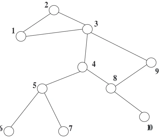
Figure 2.1: A logical network

(or intermediate) ones. For instance, in the path (1,2,3,4,5,6) of Figure 2.1, 1 and 6 are end nodes, whereas 2,3,4,5 are intermediate nodes. An end-to-end delay in the graph is the packet transmission delay over a path.

2.2.1 End-to-End Delay of the Internet

(25)

and queueing at the sender node. The propagation delay is the delay in transmitting the data packet along a physical link. In the literature, Round Trip Time (RTT) is often used to study the Internet dynamics (e.g., [70, 72]), which requires measurements only at one end. Alternatively, One-way Transmission Time (OTT) needs the collaboration at receiver to obtain the measurements. In [28] and [73], the authors found that the mean OTTs cannot be accurately approximated by dividing RTTs in half, i.e., the variations in the OTTs are often asymmetric. However because there is no guarantee to always find collaborative nodes on the Internet, RTT is still widely used in the experimental study.

2.2.2 Introduction to Prediction Theory

If a subspace M of a Hilbert space H is used to denote the information about the past of a system, a mapping that maps to an element of_Mis called apredictor [74]. Therefore _Mcan be viewed as the space of allowable predictors for the future among which we are to find the “best” one.

If ˆX is the predictor for a random variable X (X ∈_H) which represents the future, the prediction error is X−Xˆ, and it is desirable to make this error as small as possible using certain error metric. Since X−Xˆ is a random quantity and not observable in general, it is natural to pick ˆX so that X−Xˆ is small on the average. This can be done, for example, by choosing ˆX so that either Pr{|X−Xˆ| ≥ ǫ} or E[|X−Xˆ|p_{] is small, for an appropriate} value of ǫor p.

(26)

linear prediction or the Kolmogorov-Wiener prediction theory (refer to Chapter 12 of [52]) provides such a setting in which only the knowledge of the past and the first two moments of the distribution of the past are required. In fact for the normal (Gaussian) distribution, the first two moments can fully determine the distribution.

It is clear that such a prediction problem is closely related to a (quality) control problem because if we can predict how a process will behave, we can adjust the process so that the achieved values are, in some sense, as close to the target value as possible. In many applications, the purpose of predicting the Internet end-to-end packet delay is to design a working mechanism so that the Internet can work more stably and more efficiently. In particular, by more accurate prediction, delay-based bandwidth allocation and congestion control can provide further improvements to QoS in heterogeneous networks.

2.2.3 Internet End-to-End Delay Prediction: Relevant Issues

Probing Strategy

(27)

Many software tools for actively or passively measuring network performance have been developed by researchers in the fields of computer science and networking. For example,

netstat, being an important statistical tool for TCP/IP network connections, can give the current summary of the packets sent/received (with the -e option) for different protocols (with the -soption), e.g., IP, ICMP, TCP, UDP. For active probing tools,ping,pathchar [2],

NetDyn [4], traceroute are all widely used for different purposes. The CAIDA (Cooperative Association for Internet Data Analysis) website [2] provides a survey of available network measurements tools.

One important issue ought to be mentioned here is that these tools usually need cooper-ation along the routing path, e.g., response from the nodes among the path. Furthermore, several special assumptions have to hold, e.g., symmetric routing path (forward and re-verse), store-and-forward routers, nonexistence of firewalls. Being a decentralized system, the Internet has to face some uncooperative administrations and these tools might not be applicable. For example, after being attacked by the Internet worm MSBlast.D in August 2003, the servers at the University of New Orleans increased the security level of the firewall and disabled traceroute outside the firewall. In such cases, large-scale inference and Internet tomography methods [22, 30] have their special value since they can deal with uncooperative networks.

Network Tomography

(28)

Many network tomography problems can be roughly approximated by the following linear model [30]

y=Aθ+ε (2.1)

wherey is a vector of measurements, e.g., packet counts or end-to-end delays; Ais a routing matrix, θ is a vector of packet parameters, e.g., mean delays over a link, or the origin-destination traffic vector; ε is a noise term.

In the recent literature, network tomography has been divided into three classes: 1) the estimation of path-level network parameters from measurements made on individual links, which is so-called origin-destination (or source-destination) tomography (y in (2.1) is not known precisely), see, e.g., [84], 2) the estimation of link-level network parameters from path-level measurements (θ is not known precisely), see, e.g., [31, 83], and 3) topology identification (A is not known precisely), see, e.g., [33]. For the recent advanced topics in this area, see [22] for more details.

2.3 Existing Work

(29)

2.3.1 Queueing Network Modeling

A queueing system can be described as customers arriving for service, waiting for service if it is not available immediately, and leaving the system after being served [36]. The term

customer here is used in a general sense and does not imply necessarily a human customer. For example, in network modeling, a customer is a packet waiting in line to be processed. Such a basic system with a single queue can be illustrated by Figure 2.2. Using the shorthand notation introduced by Kendall (for details, refer to [36]), this is a G/G/1 queueing model.

Service facility Customers arriving

Discouraged customers leaving

Served customers leaving

Figure 2.2: A typical queueing process

Queueing theory was developed to provide models to predict the behavior of systems that attempt to provide service for randomly arising demands. Telephone traffic load analysis is one of the earliest problem studied by it.

(30)

distribution can be easily calculated.

Queueing network theory can be applied if the distribution at each individual link is known. This assumption might hold in a small-scale network with a few interconnected servers, but usually not for large-scale networks. Even though the distribution of each link is available, the computational cost will grow dramatically as the size of network increases. In addition, the product-form solution does not characterize some features of the real-life network such as the correlations introduced when traffic streams merge and split, the regu-lation of traffic by routing and flow control mechanisms, or the packet losses due to buffer overflow [18]. Due to these limitations to obtain the dynamic behavior of the networks by queueing theory, we will focus on simulation or measurement based approaches instead of such an analytical method.

2.3.2 System Identification Approach

System identification (SI) is used for building dynamic mathematical models based on the observations of the systems [60]. The three essentials in constructing models from data are: observations, candidate model sets and evaluation criteria.

Basically, for a dynamic system, we choose the observation signals we are interested in as

outputs, the external signals which can be controlled asinputs, and the others asdisturbances. Figure 2.3 is a general framework of a dynamic system [60], where y denotes the output, u

(31)

describes the effect of the probing packets. And the disturbance waccounts for effects from other traffic (i.e., packets coming from other hosts), usually modeled as white Gaussian noise (WGN).

y

u

w

Figure 2.3: A system - output y, input u, disturbance w

Then we select a candidate model set and we determine the “most” suitable one in the set for the system based on the observed data. By choosing a model fitting criterion, we can compare the models in the set to find the one that best fit the measured data. At last we do

model validation, usually based on “fresh” (new) data, to decide whether the “best” model is good enough for fitting the new observations for our purpose.

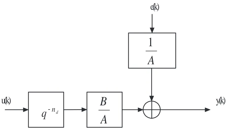
For either prediction or control purpose, the core work is to identify a model for the system (or process) given the observations on the input and output of the system. Although recently there has been an increased interest in time-varying and non-linear systems, much of the literature assumes that the system can be adequately approximated over the range of interest by a linear model whose parameters do not change with time. For instance, in [70] and [69], the authors used Auto-Regressive eXogenous (ARX) models for the delay dynamics.

As shown in Figure 2.4, a discrete-time ARX model is defined as

(32)

q

-A

1 A

B

u(k)

e(k)

y(k)

d

n

Figure 2.4: ARX model structure where A(q) and B(q) are given by

A(q) = 1 +a1q−1+· · ·+anaq

−na

B(q) = 1 +b1q−1+· · ·+bnbq

−nb

Here e(k) is unmeasurable disturbance (i.e., white noise), andq−1 _{is the delay operator;}

i.e., q−1_f₍_k_{) =}_f₍_k₋_{1). The numbers} _n

aand nb are the orders of polynomials. The number

nd corresponds to delays from the input to the output. In such a case, the adjustable parameter is

θ= [a1, a2, ..., anq, b1, b2, ..., bnb]

T _(2.3)

The “AR” in ARX models stands for the autoregressive partA(q) ande(k), and “X”denotes the external input B(q)u(k).

There are two basic methods for model fitting on observations [60]. One is the so-called

(33)

It contains famous methods such as Least Squares (LS), Maximum Likelihood Estimation (MLE), and Maximum A Posteriori (MAP) estimation, MMSE, etc. To implement these methods, adaptive filtering techniques can be applied. The other one is the Correlation Approach. Its major difference from PEM is that it does not assume prediction error is independent with the past data. Its typical methods include Instrumental-Variable method (IV) and rational transfer function model, etc. We can regard PEM as a special case of the Correlation Approach. For the problem addressed here, PEM will be emphasized.

2.3.3 Time Series Approach

A time series y(t) is a set of observations ordered sequentially in time [63]. A series of T

observations can be viewed as a random process of the variables y1, y2, ..., yT, sampled at equidistant time intervalst1, t2, ..., tT. In fact, a time series can also be treated as the output of a dynamic system whose external input cannot be observed [60].

There are two major aspects to the study of time series – analysis and modeling. The aim of analysis is to summarize the properties of a series and to characterize its salient features. This can be done either in time domain or in frequency domain. The two forms of analysis are complementary rather than competitive: The same information is processed in different ways, which provide different insights into the essence of the time series.

(34)

In time series approach, ARMA (Auto-Regressive Moving Average) models are widely used for prediction purpose. Most time series data of Internet end-to-end delay are non-stationary. However, ARMA models are used for stationary time series. This does not present an insolvable problem, since there are several methods which allow us to transform a non-stationary series into a stationary one. In most practical cases first and second-order differencings are sufficient to remove any kind of trend existing in a time series [63]. The ARIMA (Autoregressive Integrated Moving Average) methodology, developed by Box and Jenkins, is based on such an idea [19]. An ARMA model can be viewed as a special case of ARIMA models. From an engineer’s point of view, differencings in ARIMA models act as high-pass filters on the trended data.

In addition to non-stationarity in the mean of time series, we can also have non-stationarity in variance. The latter can become stationary by transforming the data into a logarithmic scale or a fraction of a power (e.g., square root).

Recent studies have revealed a fractal-like structure of delay sequences, which may not be well suited to ARMA models [49]. In [49], the authors propose a delay-boundary prediction algorithm based on a deviation-lag function (DLF) to characterize the end-to-end delay variations. Preliminary experiments show that it has an significantly increased prediction accuracy than Jacobson’s algorithm in [43], which is based on an ARMA model.

(35)

State-space models for a time series problem is usually arrived at through a structural analysis of its components that make up the series. These components may include trend, seasonal, cycle, together with explanatory variables, interventions, outliers and missing val-ues. By determining the state of the system, the useful information for prediction can be summarized efficiently. In contrast, the ARIMA modeling is a passive black box approach in which model identification relies solely on the data without prior information of the sys-tem that generated the data. Which tool is more suitable for our purpose? From a control engineer’s viewpoint, state-space models have more structural advantages than the ARIMA framework. But in the study of the Internet end-to-end delay, unfortunately, there is very little information to build up the state of the system due to the complexity of the net-works. A trade-off between these two schemes is to find the best fit time series model by the ARIMA methods first, and then convert to the state-space representation so that prediction and control can be done more efficiently.

2.3.4 Learning and Prediction

(36)

NNs are computing architectures that consist of massive parallel interconnections of simple neural processors. In fact, the NN is more like a computing technique than a new model.

The NN approach can be used in system identification and prediction, that is, we can use NNs to substitute for other forms of dynamic functions (e.g., time series). For a non-linear function, it is more useful: due to the strong adaptive learning ability of NNs, usually we can obtain a good result. NNs can also be used to construct an input-output structure. For the situation where suitable models are not available, the NN approach is invaluable since it performs a task that many other approaches can not. In such a sense, we can regard the NN method as a “blind” model.

In [72], Parlos presented an empirical approach for the identification of the end-to-end delay and round trip time dynamics using recurrent NNs. Similar to the SI approach in [70], by using the packet inter-departure time as the input and the end-to-end delay variation and round trip time variation as the output, a SISO system was built for the Internet delay dynamics. The predictors were designed for multi-step-ahead accuracy within a finite horizon.

(37)

2.4 Preliminary Data Analysis

In the literature, Round Trip Time (RTT) has often been used to study the Internet end-to-end delay dynamics (e.g., [70, 72]), which requires measurements only at one end. In [43], Jacobson designed his congestion avoidance algorithm by modeling each RTT sequence based on a certain ARMA model. Following a similar idea, we constructed an experiment to get the Internet end-to-end delay data (RTTs) and did some preliminary data analysis.

2.4.1 Data Collection

In this study we sent probing packets using Internet Control Message Protocol (ICMP) instead of TCP in [43]. More specifically, as in thepingprogram, the source host sends out a series of ICMP Echo Requests to the destination host, and the destination host returns ICMP Echo Reply messages. Here an ICMP Echo message is regarded as a probing packet. The originalpingprogram sends packets with fixed time interval (one second). We modified it so that variable inter-departure times can be obtained [88]. The reason that we chose ICMP rather than TCP is the following: TCP has an embedded congestion control mechanism so that the packet inter-departure time, which is usually considered as the system input, is not independent, identically distributed (i.i.d.) in time. However this independence assumption is required in most system identification techniques. On the other hand, User Datagram Protocol (UDP) and ICMP have no feedback-based control. The packet inter-departure time of UDP and ICMP can be freely adjusted by the end users.

(38)

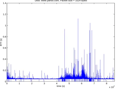
included 2 inside the LAN (without switch and with one single switch) and 6 outside the LAN (with multiple routers/switches). For each destination, we collected the RTTs as a time series using our modified ping program. Two different probing packet sizes (512 bytes and 1024 bytes) were used in the experiment, that is, for each destination there are two sets of time series data. The timeout as well as inter-departure time were set to 0.5 second. The data collection for each path lasted around 24 hours. Figure 2.5 shows one set of time series data collected from a remote destination (www.yahoo.com). Note that an RTT value of zero indicates where the packet was lost. The plot actually follows the people working pattern: the dark part (with longer delays by average) corresponds to the daytime; the flat part corresponds to the nighttime.

2.4.2 Packet Loss

(39)

0 1 2 3 4 5 6 7 8

x 104

0 0.2 0.4 0.6 0.8 1 1.2 1.4

time (s)

RTT (s)

Dest: www.yahoo.com, Packet size = 1024 bytes

Figure 2.5: A set of end-to-end delay data: the RTT sequence collected at the same host from one particular destination

about delay (RTT might not reflect traffic delay if the packet size is too small). On the other hand, the probing packets should not be too large, otherwise they may significantly affect the traffic.

2.4.3 Round Trip Times

(40)

Table 2.1: Packet loss rate

Index Target bytes= 512 bytes = 1024 A enee613-2000.uno.edu <0.0001 <0.0001

B www.sina.com 0.0273 0.0325

C www.utd.edu 0.0104 0.0112

D www.yahoo.com 0.0174 0.0176

E www.uno.edu 0.0020 0.0017

F www.google.com 0.1160 0.1698 G www.wenxuecity.com 0.0081 0.0080 H 216.107.90.145 0.0110 0.0111

Test for Stationarity

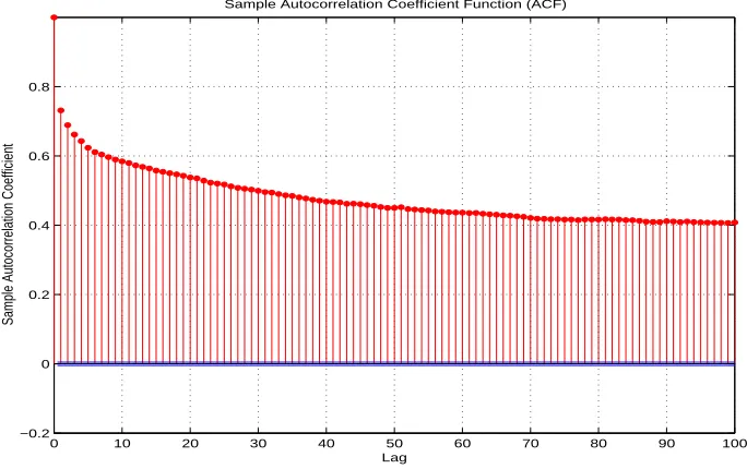
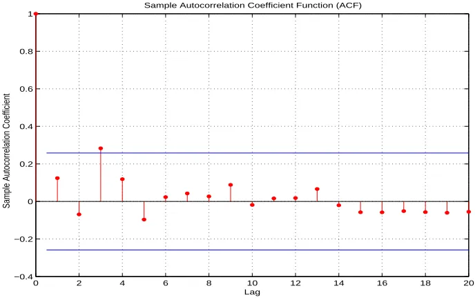
A random process is (wide sense)stationary if it has a constant mean and the autocorrelation coefficient Function (ACF) depends only on time differenceτ = ∆tbut not the absolute time

t. In time series analysis, the stationarity property leads to great simplification. Therefore the first step in time series analysis is to check whether the data are stationary or not. There are two general classes of approaches for stationarity testing, parametric and nonparametric. Being a class of totally data-driven approaches, nonparametric tests are more applicable for our case than parametric ones which often require certain model assumption. On the other hand, nonparametric tests require more data than parametric ones to achieve the same statistical decision at the same confidence level.

(41)

0 10 20 30 40 50 60 70 80 90 100 −0.2

0 0.2 0.4 0.6 0.8

Lag

Sample Autocorrelation Coefficient

Sample Autocorrelation Coefficient Function (ACF)

Figure 2.6: The sample ACFs of an RTT time series for the whole sequence The sample autocovariance function (ACVF) is given by

cτ = 1

K

K_X−τ

i=1

(zi−z¯)(zi+τ−z¯), τ = 1,2, ... (2.4) whereK is the length of the datahzki, ¯z is the sample mean of the hzki. The sample ACF is

rτ =cτ/c0 (2.5)

where c0 = _K1qPKi=1zi2·

PK−τ

(42)

0 2 4 6 8 10 12 14 16 18 20 −0.4

−0.2 0 0.2 0.4 0.6 0.8 1

Lag

Sample Autocorrelation Coefficient

Sample Autocorrelation Coefficient Function (ACF)

Figure 2.7: The sample ACFs of an RTT time series for a short time interval (60 samples)

However, such ACF analyses highly depend on experience. For example, under what rate the decay can be viewed as quick is not well defined. There is a lack of quantitative ways to make decision based on ACF plots. Therefore an alternative approach is preferred.

(43)

different observation sizes are given in Table A.6 of [15]. The runs test can be used to test stationarity as follows.

1. Divide the sequence into time intervals of equal length. 2. Compute a mean value for each interval.

3. Count the number of runs that the mean value in every interval is above (+) or below (−) the median of the whole sequence.

4. Compare the result to the known sample significance interval: if it is inside the interval, the time series is stationary; otherwise non-stationary.

When the runs test was applied to the whole sequence of a time series (e.g., data from

yahoo.com), we divided the sequence into 100 equal intervals and the number of runsr= 10. Since the 95% significance interval for 100 is [42,59], the time series isnon-stationary. To check the stationarity in shorter time ranges, we cut the whole sequence of the time series into segments with certain lengths K′_{, and treat them as different realizations of a random}

process to perform runs test one by one. When the frequency f with which the number of runs r falls inside the significance interval is high enough (say, over 90%), the time series is considered stationary with time rangeK′_.

Table 2.2: Runs test in short time ranges

Time range (samples) 30 60 90 120 · · ·

(44)

Table 2.2 shows the testing results in different time ranges. For each runs test, the data segment was divided into 10 equal length intervals and the corresponding 95% significance interval is [3,8]. From Table 2.2 we can see thatf increases as the time rangeK′ _decreases.

Although the time series is non-stationary in long-range, when the time range is smaller than 60 samples (i.e., half a minute), each data segment can be viewed as stationary sincef >90%. In other words, the time series is short-term stationary. Based on this understanding, the time series analysis will be performed in each segment with a time range around 60 samples.

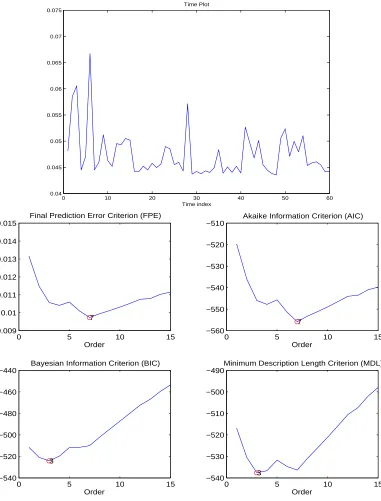
Model Order Selection in Short-Term Time Series Analysis

For the sake of the simplicity and extensity, we performed AR modeling for each data seg-ment. One primary work in AR modeling is order selection. This problem can be formulated as a testing problem of multiple composite hypotheses. Let Hn denote the hypothesis that the model order is n, where n is upper bounded by N, i.e., n ∈[1, N]. We assume that the hypotheses {Hn} are mutually exclusive meaning that only one of them can be true at one time. Note that the hypotheses {Hn} are nested since AR(n) includes AR(m) as a special case if n > m. If we only perform likelihood ratio test (or MAP with equiprobable prior), the trend of the order selection is to pick the one with the highest order, especially when the truth is not in the hypotheses. Hence there should be one penalty term which accounts for the model complexity in a “fair” model order selection rule.

LetzK _{denote a vector of} _K _{independent observations, and}_θ

n the AR parameter vector, i.e., θn = [ a₁ · · · a_n ]′. Most commonly used model selection criteria can be written in a general form

(45)

0 10 20 30 40 50 60 0.04 0.045 0.05 0.055 0.06 0.065 0.07 0.075 Time Plot Time index

0 5 10 15

0.009 0.01 0.011 0.012 0.013 0.014 0.015 7 Order

Final Prediction Error Criterion (FPE)

0 5 10 15

−560 −550 −540 −530 −520 −510 7 Order

Akaike Information Criterion (AIC)

0 5 10 15

−540 −520 −500 −480 −460 −440 3 Order

Bayesian Information Criterion (BIC)

0 5 10 15

−540 −530 −520 −510 −500 −490 3 Order

Minimum Description Length Criterion (MDL)

(46)

minimized among N hypotheses. Here log denotes the natural logarithm and ˆθn is the maximum likelihood (ML) estimate

ˆ

θn= arg max θn

fn(zK|θn) (2.7) The first term of ξn in (2.6) is a natural extension of the generalized likelihood test (GLRT) to deal with multiple hypotheses testing. The reason we add a multiplier 2 is to cancel the factor 1/2 under Gaussian assumption. Due to the limited data and the model nesting issue, if only this term is used for model selection, we will usually have an overfit. Thus the second term dn(zK) is used as a penalty function that varies for different criteria. The Akaike information criterion (AIC) usesdn(zK) = 2n[5]. The Bayesian information criterion (BIC, also known as SBC – Schwartz’s Bayesian Criterion) uses dn(zK) =nlogK [78]. The minimum description length (MDL) criterion uses dn(zK) = 2 log(

R

fn(zK|θˆn)dzK) which is interpreted as part of the normalized maximum likelihood (NML) [76]. Akaike’s final prediction error (FPE) criterion uses dn(zK) = 2Klog[(K+n)/(K−n)] [60] 1.

In general, the penalty terms have the order: FPE ≈ AIC <BIC ≈ MDL. When obser-vation numberK goes to infinity, BIC (and MDL) can select the best model asymptotically with probability 1 given that the truth is in the model set [78]. FPE and AIC do not have this asymptotic property; they always overfit the data, especially when the sample size is small. Figure 2.8 shows an example in which we used different criteria to decide the AR order of a segment from the time series data.

We applied the above model selection criteria to the whole time series data to take a glance at the model structure. To satisfy the stationarity constraint, the time series data

1_{Rigorously speaking, this is the form of log(FPE). Originally, FPE was defined using prediction error}

(47)

have to be segmented into small pieces to perform analysis. The segment size was chosen to have 60 samples (i.e., half a minute). Sliding windows were used in segmentation to reduce the impact due to high frequency components. A sliding window is like a stencil that you move along a data stream, exposing only a fixed number of data points at one time. Here the window size was 60 samples. The window moving step (sliding factor) was 30 samples, that is, there were 60−30 = 30 samples overlapping between the adjacent segments.

0 10 20 30

0 2000 4000 6000 8000 Order FPE

0 10 20 30

0 2000 4000 6000 8000 Order AIC

0 10 20 30

0 0.5 1 1.5 2 2.5x 10

4

Order BIC

0 5 10 15 20 25 0

0.5 1 1.5

2x 10

4

Order MDL

Figure 2.9: The histograms of model selection results

(48)

models with order 4 or lower. Therefore the orders of AR models in the short-term time series analysis were chosen as 4 or lower. For simplicity, the orders of all the AR models can be further approximated to be 4 (AR models of a lower order can be viewed as special cases of AR(4) models) to accomplish some batch work.

2.5 The Multiple-Model Approach

Based on the preliminary data analysis, we concluded that the Internet end-to-end data can be analyzed by AR modeling in each short data segment [90]. However, even though the structure (order) of each model can be chosen as the same, the parameters in different seg-ments are usually different. How to use these different AR models to do prediction? Bayesian framework is a natural choice. More specifically, the multiple-model (MM) approach is par-ticularly suitable to this situation since it could solve the model selection problem and parameter estimation problem jointly.

2.5.1 Multiple-Model Predictor

(49)

Model 1 Filter Model 1

Filter Model 2

Filter Model M

Filter Model M Filter

Cooperation

Filter Output Fusion (Combination)

Overall Estimate Data

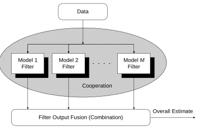
Figure 2.10: General structure of multiple-model methods

A general structure of multiple-model methods is given in Figure 2.10. Development of an MM predictor consists of the following steps: model set design, filter selection, cooperation strategy development, and estimate output fusion. Here “cooperation” means any actions taken among the filters to achieve better performance, such as individualized recondition-ing of each filter (e.g., in the interactrecondition-ing MM (IMM) algorithm), interactive iterations and competitions (e.g., in EM based algorithms), etc. The final step, estimate fusion, can be achieved by a procedure based on hard decision or soft decision (e.g, weighted sum). A more detailed description of the MM methods can be found in [51, 55].

(50)

lit-erature under various other names, such as “multiple model adaptive estimator/filter” [14], “multi-model partitioning algorithm” [47], etc. However, as a consequence of its underly-ing assumption, this method is not effective in handlunderly-ing systems with frequent mode jumps (which is likely in the Internet end-to-end measurements) because without any interaction among filters it will take a considerable amount of time for the overall estimate to converge to the true mode. Unlike AMM, the IMM estimator assumes that the system mode is a Markov (or semi-Markov) process and thus is allowed to jump between members of a set. In the IMM algorithm, each filter uses a weighted sum of the most recent estimates from every filter as its input which usually differs from one to another. By such a cooperation, IMM can capture the mode transition faster than AMM.

Most existing MM algorithms are built on state-space models and a Kalman filter (KF) is run for each model (for a nonlinear case, an extended KF (EKF) can be used). Note that based on the same idea MM algorithms can also be derived using filters in other forms (e.g., ARMA). The KF was picked mainly because of its simplicity among its peers and capability of on-line recursion.

We apply the IMM algorithm to predict the Internet end-to-end delay. Figure 2.11 shows the block diagram of the IMM algorithm. Note that each filter input matching the corresponding mode is obtained through a mixture of all filter estimates at the previous time. This operation is what “interacting” stands for. A complete cycle of the IMM scheme with Kalman filter as its mode-matched filter is summarized in Table II of [55]. The most widely used minimum mean square error (MMSE) linear predictor is applied in our approach. Let

zk _,_{_z

(51)

2 1 | 1 − − k k

x

Model 1 based filter

Model 2 based filter

Model M based filter

In

te

ra

c

tio

n

E

s

tim

a

tio

n

F

u

s

io

n

…

output

M k k

x

₋₁_| ₋₁

1 |

ˆ

_k_k

x

2 |

ˆ

_k_k

x

M k k

x

ˆ

_|

1 1 | 1 − − k k

x

k k

x

ˆ

_|

k

z

Figure 2.11: The block diagram of the IMM algorithm then the MMSE linear predictor is

ˆ

The model set is constructed from different AR models (to be presented later). We choose AR models since they have a simple structure and can approximate well a large class of short-term stationary data. To implement the IMM algorithm, the above models should be converted to the state-space representation [88]. Consider an AR(p) model

zk+a1zk−1+· · ·+apzk−p =b0ωk (2.9)

where hωkiis a white noise sequence. Let M denote the set of all M designed models andj a generic model in it. Then each AR(p) model can be represented by

xk+1 =F_kjxk+Gj_kω_kj (2.10)

(52)

where x is the state vector; z is the measurement vector; ωk ∼ N(0, Q) and υk ∼ N(0, R) are independent process and measurement noise, respectively; and the initial state x0 ∼

N(x0, P0) is independent ofωkandυk. The model matrices (F,GandH) can be determined in the observable canonical form:

F =                

−a1 1 0 · · · 0

−a2 0 1 · · · 0

..

. ... ... . .. ...

−ap−1 0 0 · · · 1

−ap 0 0 · · · 0

               

, G=−                 a1 a2 .. .

ap−1

ap                

b0 (2.12)

H =

1 0 0 · · · 0

It is assumed that the system mode sequence is a first order Markov chain with transition probabilities πij = P{mj_k₊₁|mik}, where mik denotes that the ith model is in effect at time

k. In MM, (posterior) model probabilities provide a meaningful measure of how likely each mode is at a given time. It can be used as a measure for detection of process jumps by comparing some preset thresholds. An l-step ahead end-to-end delay predictor is

b

zk+l|k = n

X

j=1

b

zj_k₊_l_|_kµj_k₊_l_|_k (2.13)

Pk+l|k= n

X

j=1

µj_k₊_η_|_k= n

X

i=1

πijµik+η−1|k (2.15) where bzj_k₊_l_|_k is the predicted delay estimate from thejth elemental filter,µj_k₊_l_|_k is the corre-sponding model probability which can be obtained by running (2.15) from η = 1 to l, µi

(53)

is the i-th model probability of the state estimate ˆxk, and n is the number of models in the model setin effect at timek. (2.13) uses the total expectation theorem to obtain the overall estimate bzk+l|k based on all predicted measurement estimates.

2.5.2 Model Set Design

Model set design is the most important part in the implementation of the MM methods. The performance of MM methods depends largely on the set of models chosen for the problem. A theoretical discussion of model set design can be found in [57, 55]. In this paper, based on preliminary data analysis, an off-line VQ-based method is proposed, which can be viewed as a special case of the clustering method in [57].

Vector Quantization and Clustering

Vector quantization (VQ) is a (usually lossy) data compression method based on the principle of block coding [62]. A VQ is nothing more than an approximator. The idea is similar to that of “rounding-off” (say, to the nearest integer). It is more effective than scalar quantization (can achieve less than 1 bit/parameter).

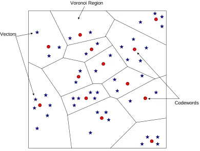
VQ has deep roots in the clustering algorithms. Clustering is an example of unsupervised learning. Usually, the number and form of classes {Ci} are unknown, and available data samples {xi} are unlabeled. VQ can be viewed as a special case of clustering (K-means [27] clustering). From this point of view, each individual cluster centroid in VQ is called a

(54)

Codewords Vectors

Voronoi Region

Figure 2.12: Codewords (clustering center) in 2-dimensional space, where the Voronoi regions (nearest neighbor regions) are separated with boundary lines

The LBG Algorithm

VQ can be formulated as an optimization problem. There are two optimality conditions that must be satisfied:

• Nearest neighbor condition: usually used with a Euclidean distance metric

d(x, y) =||x−y||2 _{= (}_x₋_y₎′

(x−y) (2.16)

(55)

In 1980, Linde, Buzo, and Gray (LBG) proposed a VQ design algorithm based on a training sequence [58]. The LBG VQ design algorithm is an iterative algorithm which alter-natively solves the above two optimality criteria. In this method, an initial codeword is set as the average of the entire training sequence. At the beginning, the initial codeword is split into two. The iterative algorithm is run with these two vectors as the initial codebook. After iteration, the two obtained codewords are splitted into four and the process is repeated until the desired number of codewords is obtained. Further details of the LBG algorithm can be found in [58].

Model Set Design Procedure

Time Series

AR( p) models Short-term

analysis Raw data

Quantized AR models Candidate

model set MM Approach

LBG Algorithm

Vector Quantizaion Skip missing

data

State-space representation

Figure 2.13: Model set design diagram

(56)

Raw data in the diagram were chosen from the training dataset with 8 different destinations. By the same segmentation scheme in the preliminary data analysis, the training data were segmented into equal-length (60 samples) pieces. After segmentation, we did short-term analysis for each segment to get an AR model. Since there are too many models of different parameters obtained from the training set, the VQ method was used to select the candidate models. As discussed in Section 2.4.1, the order of AR models was chosen fixed at 4. In fact, this setting is just for simplicity, since after clustering, there is no guarantee that lower order AR models can be obtained although they are more suitable in many segments (refer to Figure 2.9). The parameters of each AR(4) model can be viewed as a 5-dimensional vector to apply VQ techniques. The LBG algorithm was used here. The size of the model set, i.e., the size of the codebook, was chosen to be 8. To implement the existing MM algorithms, the quantized models are converted to the state space.

2.6 Numerical Results

(57)

Least Mean Square (LMS), Recursive Least Square (RLS) are two most widely used linear adaptive filters. Here they are used as the baseline solutions whose performance is compared with that of the MM methods. The root-mean-square error (RMSE) of the end-to-end delay prediction was used as the performance measure. It is defined as

RMSE(bzk+l|k) =

v u u

t 1

N

X

i=1

(zi

k+l−zbki+l|k)2 (2.17) where N is the number of Monte Carlo runs, k is the time index, l is the prediction steps, and the superscript i stands for quantities on the i-th run.

2.6.1 Synthetic Data

Figures 2.6.1 and 2.15 show the simulation results using AMM and IMM respectively. The time series in the simulation were made up of three different order AR models: AR(1), AR(2), and AR(3). More specifically, the data sequence was generated by five segments: AR(1)-AR(2)-AR(1)-AR(3)-AR(1) in order, which are shown in the figures. All data plots are averages over 100 Monte Carlo runs. The transition probabilities in the IMM were chosen as πii = 0.90, πij = 0.05, i, j = 1,2,3, i 6=j, which means each model was viewed equally. Comparing the results of the two methods, we found that using IMM the model switchings in the sequence can be accurately tracked, whereas using AMM the delays in time to catch the model changes are relatively long. This phenomenon will be more apparent when model switchings happen more often. In the real data we collected, abrupt peaks were observed very frequently, which suggests that IMM should be a better choice than AMM.

(58)

0 20 40 60 80 100 120 140 160 −1 −0.5 0 0.5 1 Data

0 20 40 60 80 100 120 140 160

0 1 2 3 4

One−step ahead prediction

Time index

RMSE

0 20 40 60 80 100 120 140 160

0 0.5 1 Model probabilities AR(1) AR(2) AR(3)

AR(1) AR(2) AR(1) AR(3) AR(1)

Figure 2.14: Prediction using AMM with AR models of different orders

0 20 40 60 80 100 120 140 160

−1 −0.5 0 0.5 1 Data

0 20 40 60 80 100 120 140 160

0 1 2 3 4

One−step ahead prediction

Time index

RMSE

0 20 40 60 80 100 120 140 160

0 0.2 0.4 0.6 0.8 Model probabilities AR(1) AR(2) AR(3)

AR(1) AR(2) AR(1) AR(3) AR(1)

(59)

20 40 60 80 100 120 140 0.8

1 1.2 1.4 1.6 1.8 2 2.2 2.4 2.6 2.8

Iteration number

RMSE

The Average Learning Curve of Predictor

LMS

RLS(λ=1)

IMM

RLS(λ=0.9)

Figure 2.16: Performance comparison between IMM and adaptive filters (synthetic data) size µ= 0.0035 (larger µ, e.g., 0.005, will make the filter diverge); For RLS, initial constant

δ = 0.1, forgetting factor λ≤1. Note that λ= 1 corresponds to infinite memory. In Figure 2.16, case λ = 0.9 (only 10 samples in memory) has also been checked. The performance of IMM is always better than that of LMS and RLS. A short memory will make the performance of RLS worse.

2.6.2 Measured Data

(60)

constant δ= 0.1, forgetting factor λ= 1. For IMM, the transition probabilities were simply designed as πii= 0.93,πij = 0.01,i6=j.

50 100 150 200 250 300 350 400 450 500

−0.02 0 0.02 0.04 0.06 0.08 0.1

Iteration number

RMSE

The Average Learning Curve of Predictor

LMS RLS IMM

Single AR(4) model

Figure 2.17: Performance comparison between IMM and adaptive filters (measured data) The prediction results by different predictors are compared in Figure 2.17, which was zoomed in to show the difference of the flat parts of the prediction errors. Note that for the peaks, the prediction errors has the order IMM < RLS < LMS on average. The prediction interval l was chosen as 5. The prediction errors of a single AR(4) model are also shown in the figure as a baseline solution. Table 2.3 gives the average RMSE over time for different prediction intervals l, which also shows that IMM significantly outperforms LMS and RLS on average.

(61)

Table 2.3: Average RMSE comparison

l = 1 l= 2 l = 5 l = 10

LMS 0.0657 0.0642 0.0647 0.0668 RLS 0.0584 0.0570 0.0562 0.0586 IMM 0.0458 0.0471 0.0422 0.0454

be chosen carefully; otherwise they could be much worse. For example, the learning curve of LMS here converges very slowly; however, a larger µ will make the prediction diverge, and a smaller µ will decrease the convergence rate further. IMM is not so sensitive to the parameter design. In this sense, IMM is more robust than LMS and RLS.

2.7 Discussion and Conclusions

In this chapter, a novel approach to model the Internet end-to-end delay dynamics using MM methods has been proposed. Although each model is LTI, the MM method provides a non-stationary, nonlinear solution. It turned out that the proposed MM method performs better for prediction, in a highly non-stationary and nonlinear case, than two well known adaptive filters, namely, LMS and RLS.

(62)

(63)

Chapter 3 Joint Decision and Estimation

3.1 Introduction

3.1.1 Statistical Decision

(64)

waveforms, to make a decision which speaker is among a group is also an important problem (speaker identification). All the above examples can be formulated within statistical decision theory.

3.1.2 Parameter Estimation

Literally, according to Wikipedia, “Estimation is the calculated approximation of a result which is usable even if input data may be incomplete, uncertain, or noisy.” In real engineering problems, if we consider the unknown quantity to be estimated, – let us call itestimatee [52], there are two types of estimatees involved in estimation. If the estimatee is time-invariant or slow-varying, it is usually called parameter estimation; if the estimatee is rapid-varying, it is called process (or state) estimation (since we are talking about statistical random process). Another widely-used alias for process estimation is “filtering.”

The applications of estimation are also ubiquitous. Let us consider the same areas in the previous examples: In radar systems, besides determining the presence/absence of the target, at most time we also want to know relatively precisely the location, velocity, acceleration, etc. and other parameters based the observed data. In digital communications, estimating channel parameters are very important to ensure the robustness and security. In speech processing, an accurate estimate of speaker’s pitch acts as the leading role in most tasks.

(65)

estimation. This scalability issue is important since in some areas, for instance, target tracking, process estimation is more important.

3.1.3 Joint Decision and Estimation

What is the difference and relationship between decision and estimation? Let us give a more rigorous definition firstly. Estimation is an operation to select a point from a continuous space. And decision is an operation to select one out of a set of discrete alternatives [12]. In other words, they both try to make the “best choice,” one in a continuous space and the other in a discrete space. Decision can be viewed as a special case of estimation since usually we may consider a discrete space as a subspace of a continuous space. Of course people can argue the other way around. In fact, the estimation can be done in a discrete valued-case, the output is not necessarily one of the candidate values but some of them with probabilities. From this point of view, these two operations are highly related and they have an overlap.

(66)

of the candidate values, which is so-called “hard decision,” but some values obtained from different candidate values with conditional probabilities (let us call it “soft decision”). What is the difference between these two concepts? Consider a binary case with two candidates “0” and “1”. In the hard decision, the decision output is either “0” or “1”; whereas in the soft decision, the output is some value in between. As we argued before, we can even think the soft decision as one possible way to achieve estimation. The soft decision is very important in the MM method, especially useful when the true model is not included in the candidate model set (for instance, in Internet end-to-end delay modeling, it might be the case). However, in some other engineering problems, the soft decision is unacceptable, and in this chapter we will concentrate on how to solve the problems with such requirement (hard decision) in an optimal way.

(67)

Comm. Tower Fusion Center

? ?

UAV

Cloud

Wireless Sensors

Figure 3.1: Joint tracking and recognition of crossing targets

(68)

uncertain term with the maximum likelihood estimate. Usually, the decision results using GLRT are suboptimal [25]. Due to the drawbacks in these two approaches, a joint solution is preferred.

3.1.4 Existing Work

In 1968, Middleton and Esposito [66] proposed an integrated framework to solve decision and estimation jointly. They called the approach “simultaneous signal detection and estimation.” In their terms, detection and estimation are both “decision” problems since they both try to make the right decision among their problem regions. Therefore they only talked about “decision theory” which emphasizes the connection between decision and estimation. We also want to highlight the difference of the two operations, unless stated otherwise, the word “decision” is reserved for the discrete case only. From this point of view, they were handling a JDE problem and the general model they considered (they called “signal extraction”) is shown in Figure 3.2.

+

Detector

Estimator

)

,

(

t

θ

S

V

=

S

⊕

N

)

(t

N

)

(V

i

γ

)

(V

s

γ

1 , 0

=

i

Figure 3.2: A general model of detection-estimation problem

(69)

In general, the purpose of the system depicted in Figure 3.2 is to provide a double judgement (or in their word, “decision”) at its output: a detection as to the presence or absence of the signal and, possibly, an estimate of the signal waveform S, or of the signal parameters θ. This model includes, among other cases: 1) the usual detection problem when the estimator is not present; 2) the usual estimation problem when the signal is present with probability 1 in the observation interval and, therefore, no detection is necessary; and 3) a new type of estimation problem when there is no detection operation involved, but an estimate has to be made without certainty as to the presence of the signal. The main purpose of their approach is to improve the estimate accuracy: comparing with conventional approach, it accounts for possible decision errors, and decision is also affected by estimation. Their solution is based on a Bayesian setting. Since they considered the two operations identical in principle, they used a unified Bayes risk or cost R(σ, δ) in their solution.

R(σ, δ) =

Z Ω       

σ(S)

σ(θ)        dS dθ Z Γ

Fn(V|S(θ))dV

Z

∆

δ(γ|V)

      

C(S,γ)

C(θ,γ)

      

dγ (3.1) whereσ is a priori PDF of Sorθ,Fn(V|S(θ)) conditional PDF of dataV givenS;C(S,γ),

C(θ,γ) are cost functions relating decisionsγ ,(γ1, γ2, ..., γM);γin detection is in a discrete set of values (e.g., 0,1 in ON-OFF case),γin estimation is in a continuum of values; δ(γ|V) is a decision rule; Ω, Γ, ∆, are spaces for (S or θ), data V, decisions γ, respectively (here the decision is following their definition). The optimization is done in a two-stage procedure: Initially they assume that the estimator γ is assigned and determine the best detection rule

δ∗ _{(as a function of} _γ_{); then find the best estimator} _γ∗ _{that further minimizes the average}

When Decision Meets Estimation: Theory and Applications

ScholarWorks@UNO

ScholarWorks@UNO

When Decision Meets Estimation: Theory and Applications

When Decision Meets Estimation: Theory and Applications

When Decision Meets Estimation: Theory and Applications

A Dissertation

Acknowledgment

Abstract

Contents

List of Figures

List of Tables

Chapter 1

Introduction

1.1

Motivation

1.2

Hybrid Systems and Hybrid Estimation

1.2.1

Multiple-Model Methods

1.2.2

Predicting Internet End-to-End Packet Delay

1.3

Joint Decision and Estimation

1.4

Thesis Outline

Chapter 2

MM Prediction of Internet

End-to-End Packet Delay

2.1

Introduction

2.2

Problem Description

1

2

3

4

5

6

7

8

10

9

2.2.1

End-to-End Delay of the Internet

2.2.2

Introduction to Prediction Theory

2.2.3

Internet End-to-End Delay Prediction: Relevant Issues

2.3

Existing Work

2.3.1

Queueing Network Modeling

2.3.2

System Identification Approach

y

u

w

q

-A

1

A

B

u(k)

e(k)

y(k)

n

2.3.3

Time Series Approach

2.3.4

Learning and Prediction

2.4

Preliminary Data Analysis

2.4.1

Data Collection

2.4.2

Packet Loss

2.4.3

Round Trip Times

2.5