Two Essays in Business Cycle Theory

University of New Orleans University of New Orleans

ScholarWorks@UNO

ScholarWorks@UNO

University of New Orleans Theses and

Dissertations Dissertations and Theses

8-10-2005

Two Essays in Business Cycle Theory

Two Essays in Business Cycle Theory

Nazneen Ahmad University of New Orleans

Follow this and additional works at: https://scholarworks.uno.edu/td

Recommended Citation Recommended Citation

Ahmad, Nazneen, "Two Essays in Business Cycle Theory" (2005). University of New Orleans Theses and Dissertations. 297.

https://scholarworks.uno.edu/td/297

This Thesis is protected by copyright and/or related rights. It has been brought to you by ScholarWorks@UNO with permission from the rights-holder(s). You are free to use this Thesis in any way that is permitted by the copyright and related rights legislation that applies to your use. For other uses you need to obtain permission from the rights-holder(s) directly, unless additional rights are indicated by a Creative Commons license in the record and/or on the work itself.

TWO ESSAYS IN BUSINESS CYCLE THEORY

A Dissertation

Submitted to the Graduate Faculty of the University of New Orleans in partial fulfillment of the requirements for the degree of

Doctor of Philosophy in

Financial Economics

by

Nazneen Ahmad

M.S., University of New Orleans, 2005 M.A., York University, 2000

Acknowledgment

I want to express my deepest appreciation to the Chairman of my dissertation committee, Dr. Wei Xiao, who not only provided excellent guidance but also served as a mentor and role model. He earned my special gratitude for his continuous support, patience and persistent optimism. He was always there to listen, to give advice and help me think through both analytical and

computational problems.

I would like to thank my dissertation committee members Drs. Michael Morris, Atsuyuki Naka, Arja Turunen-Red and Gerald Whitney for their valuable comments and encouragements.

Table of Contents

List of Tables ...v

List of Figures ... vi

Abstract... vii

Essay 1 End of Double Taxation and Economic Recovery 1. Introduction...1

2. The Model...3

2.1 The Economy ...3

3. Calibration and System Dynamics...5

4. Quantitative Results ...8

4.1. Economic Recovery from Permanent Reforms ...8

4.2. Economic Recovery from Temporary Reforms...15

4.3. The Growth Effects...18

5. Sensitivity Analysis ...20

6. Conclusion ...23

Essay 2 Prospect Theory and the Welfare Cost of Business Cycles 1. Introduction...24

2. The Prospect Theory and Consumer Preferences ...27

3. The Framework...29

3.1. Consumer Preferences ...29

3.2. Measuring Gains and Losses ...30

3.3. Utility from Gains and Losses ...30

3.4. Welfare Cost Estimation ...31

4. Computation and Quantitative Results ...33

5. Sensitivity Analysis ...36

6. Conclusion ...39

References...41

List of Tables

Table 1. Parameter Values of the Benchmark Model ...7

Table 2. Long Run Changes in the Levels...9

Table 3. Sensitivity Analysis ...21

Table 4. Welfare Costs of Fluctuations in Asset Returns ...35

Table 5. Welfare Costs with CRRA Prospective Utility Function ...38

List of Figures

Figure 1A. Transitional Dynamics of Output ...9

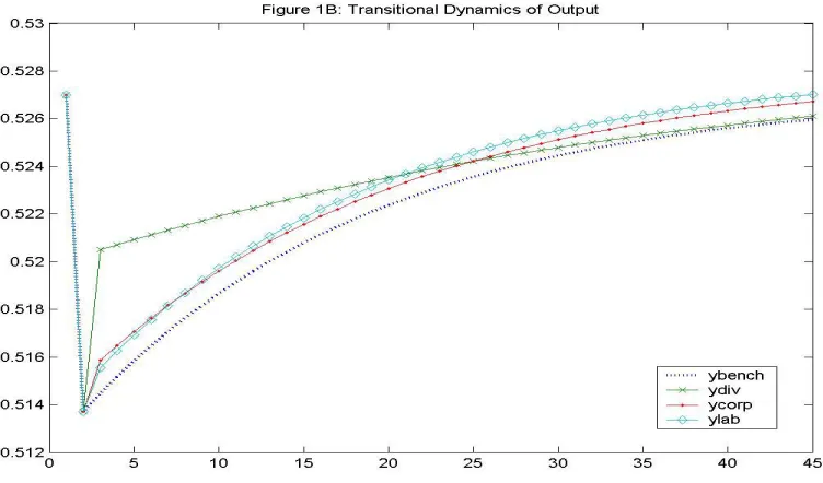
Figure 1B. Transitional Dynamics of Output ...10

Figure 2A. Transitional Dynamics of Investment...11

Figure 2B. Transitional Dynamics of Investment...12

Figure 3A. Transitional Dynamics of Employment...13

Figure 3B. Transitional Dynamics of Employment...13

Figure 4. Transitional Dynamics of Government Expenditure...14

Figure 5. Transitional Dynamics of Output ...15

Figure 6. Transitional Dynamics of Investment ...16

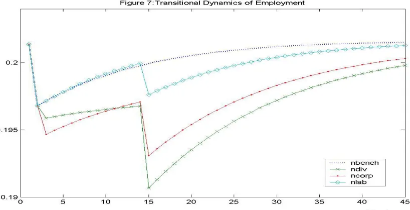
Figure 7. Transitional Dynamics of Employment...17

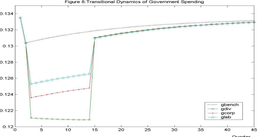
Figure 8. Transitional Dynamics of Government Expenditure...18

Figure 9. Growth Rate of Output ...19

Figure 10. Growth Rate of Output ...19

Figure 11. Real GDP and S & P 500 Composite Index...26

Figure 12. Utility Function Supported by the Prospect Theory...28

A

bstract

This dissertation studies two interesting business cycle issues. The first issue concerns the

effectiveness of tax policies in stimulating an economic recovery. The second issue concerns the

costs of business cycle fluctuations to an investor who chooses to invest in risky assets.

The first essay evaluates the effectiveness of the “end of double tax” policy in stimulating

an economic recovery by analyzing the transitional dynamics of the economy’s aggregates

toward the steady states. The effectiveness of this policy is compared with two alternative

policies that reduce corporate income or personal income taxes. Although all of these tax policies

are found to stimulate the economy’s levels of output and investment, the “end of double

taxation” appears to exert the most significant impact on the aggregate levels of these variables

in the short run. Based on this finding, we claim that the “end of double taxation” is an effective

policy for stimulating an economic recovery in the short-run.

In a thought-provoking exercise Lucas (1987 and 2003) argues that the welfare costs of

business cycles is negligible. The second essay follows up on this argument by incorporating

prospect theory into the formulation of individual preferences. Prospect theory proposes that

agents care about changes in their wealth level rather than the level of their final wealth, and

individuals are also taken to be more sensitive to losses than gains in their financial wealth.

According to the prospect theory, therefore, the agents take fluctuations in the asset returns

2.58-9.49% of the average returns, she receives from investing in the risky asset, in order to

eliminate all the fluctuations associated with her asset returns. This result is interpreted as an

Essay 1: End of Double Taxation and Economic Recovery

1. Introduction

The long-run impact of capital income taxation on the economy has been extensively studied in the literature. In Chamley (1986)’s seminal work, for example, the optimal rate of capital income tax is shown to be zero in the steady state of a general equilibrium model without uncertainty. Zhu (1992) and Chari et al. (1994) show that a similar conclusion holds for a

stochastic version of the economy. Lucas (1990), on the other hand, shows that if the capital income tax is eliminated and all the government revenues are raised from the labor income tax, the long-run growth rate of capital stock and output will increase significantly. Devereux and Love (1994) and I&mrohorog(lu(1998) present similar results for economies with human capital and with over-lapping generations.

Few researchers, however, have paid much attention to the short-run dynamics associated with the changes in the capital income tax rate. In particular, when the economy temporarily deviates from its long-run growth path and falls into a recession, can the capital income tax rate be used as an effective tool to speed up the economic recovery? How does it compare with other policy measures such as labor income taxes? This issue has become particularly interesting within the context of a recent policy change. In May 2003, the congress passed the “Jobs and Growth Tax Relief Reconciliation Act,” in which it promised to eliminate the tax on dividend income of the investors retroactive to January 1, 2003 through December 31, 2008. The declared goal of the act was to “speed up an economic recovery by encouraging consumer spending and promoting private sector investment.” Clearly, the law was very much focused on achieving short-term economic objectives.

reinvested in the firm. This cumulative tax on retained earnings is up to 48%. If the double taxation on capital income is eliminated, a company would pay tax on its profit at the statutory corporate tax rate, but there will be no tax on the investors’ dividends. Policy-makers expect that the “end of double taxation” on capital income would promote capital formation by encouraging the private sector to invest and in turn generate a fast economic expansion.

In this paper, we evaluate the effectiveness of the “end of double taxation” policy as a tool for stimulating economic recoveries. Specifically, we study a real business cycle model in which firms are subject to the double taxation system similar to the one we just described. In period one, a negative and persistent shock “drags” the economy into a temporary recession. Then, in an attempt to end the recession, the government eliminates the double taxation on capital income. We evaluate the impact of this policy by analyzing the transitional dynamics of the aggregate variables towards the steady states. We consider both a “temporary policy” that eliminates dividend taxes for only 3 years and a “permanent policy” that eliminates dividend taxes forever. We also compare the effectiveness of this policy with two alternative policies that reduce labor income and business income taxes. A policy is desirable if it leads to a fast

transition back to the steady state and causes the least loss of output in a given period of time. Lucas (1990), Devereux and Love (1994) and &Imrohorog(lu (1998) also study the quantitative effect of capital income taxes in general equilibrium models. Using endogenous growth models, they are able to identify the impact of this policy on the long-run growth rate of the economy. Therefore, their focus is on the “growth effect” of capital income taxes. The model environment we consider is a neo-classical economy where the growth rate of the economy is deterministic. Eliminating dividend taxes has no growth effect in this environment. Instead, there will be a “level effect” which is reflected by changes in steady state output and other aggregate variables. The transition dynamics from one steady state level to another is the focus of this study, since such dynamics shed light on how the economy recovers from a recession with the help of alternative tax policies.

compared to those for two other policy reforms. However, the economy’s long run employment is stimulated only when the personal income tax rate is reduced permanently.

The rest of the paper is organized as follows. The model is presented in section 2. Section 3 presents the parameter values of our benchmark economy and the mechanism that generates the transitional dynamics of the economy. Quantitative results are provided in section 4. Section 5 tests the robustness of our results. Section 6 concludes the paper.

2. The Model

We consider a decentralized neoclassical economy. The economy consists of three-sectors: households, firms and the government. The households own the firms and receive profit from the firms in the form of dividends. The firms produce a unique good, which can be either consumed in the current period or transformed to physical capital in the next period. The government taxes the private sector on their earnings from labor as well as capital services to finance its spending.

2.1 The Economy

There are a large number of infinitely lived identical individuals in the economy. The preferences of the representative household are of the following form:

lnl_t)

0

t (lnct t

max ∑∞ θ

=β + , (1)

where 0<β<1 is the discount factor, θ represents preference for leisure, and ct and lt are

consumption and leisure per capita. The utility function is strictly increasing, concave, and twice continuously differentiable.

The household splits total time between work and leisure activities. Normalizing the total time endowment to one, the time constraint takes the following form:

1

= + _t

t l

n (2)

The household receives wages at a rate wt for each unit of labor supplied and rent at a rate

rt for each unit of physical capital (kt) supplied to the firm. In addition, as the owner of the firm,

he receives dividend from the firm. The household pays taxes on all these incomes at three different rates. Thus the budget constraint of the household is

and the tax bill paid by the household at each period of time is as follows:

t_t =τ_pw_tn_t +ητ_d[(1−τ_b)(r_tk_t −φ_ki_t)]+τ_b(r_tk_t −φ_ki_t), (4)

Whereτ_p>0, τ_d>0 and τ_b>0 respectively are the rates at which wages, dividends and profits are

taxed. The index,η∈

[ ]

k

ϕ represents the fraction of investment that is deducted from the firm’s taxable income. This

fraction of deduction from the business taxable income represents an element of the U.S. tax code that provides incentive to the private sector to invest.

The firm combines physical capital and labor, to produce the final good, using the following production technology:

α − α =A_tk_t n1_t t

y , (5)

Where α represents the share of capital in total output. At represents the random productivity

shock variable, which follows AR(1) process, given by:

t t

t A

A₊₁ = ρ +ε , (6)

Where 0<ρ<1 is the persistence parameter and ε~ N(0, 2

ε

σ ).

The capital accumulation of the economy occurs through the following dynamic constraint: t k ) 1 ( 1 t k t

i = ₊ − −δ , (7)

where δ is the rate of capital depreciation.

In equilibrium, profit maximization by the firm implies that both factors are paid their marginal products. Thus we have the following:

t t t

k y

r =α , (8)

t t t

n y

w =(1−α) (9)

Given the associated constraints the household chooses consumption, leisure, and capital to maximize her lifetime utility, which yields the following necessary conditions for equilibrium:

_t

t

c =λ

1

(1 ) (1 ) 1 p t t t t n y

n λ α τ

θ _{= − −}

− , (11)

] ) 1 ( )][ ) 1 ( ( 1 [ )] ) 1 ( ( 1 [ k y t 1 t b b p k b b p 1 t 1 t 1

t − τ η −τ +τ = −φ τ η −τ +τ β −δ λ −λ

αβλ ₊

+ +

+ , (12)

Where λ is the Lagrange multiplier associated with the household’s budget constraint.

Equation (10) equates the marginal utility of consumption to its opportunity cost (λ_t). Equation (11) equates the marginal disutility of supplying labor to the after-tax real wage. Equation (12) equalizes the post-tax marginal costs and benefits of investing in future capital.

The government sets the tax code parametersτ_p,τ_d, τ_b,ηand ϕ_kto raise a specific level of per capita government revenue each period. Government revenue, gt, does not contribute to

either production or individual utility. For simplicity, we assume that the government budget is balanced each period. The budget constraint of the government is defined as follows:

) i k r ( ) i k r )( 1 ( n w

g_t =τ_{p t t} +ητ_d −τ_{b t t} −φ_{k t} +τ_{b t t} −φ_{k t} . (13)

A dynamic equilibrium of the economy consists of the sequences

{

}

The household’s budget constraint (3) and the government’s budget constraint (13) yield the following market clearing condition for the economy:

t g t i t c t

y = + + . (14)

3. Calibration and System Dynamics

Most parameters are calibrated to be consistent with existing findings in the literature. Sometimes we vary some parameters around our initial benchmark settings for robustness check purposes.

King and Rebelo (2000)[henceforth KR] set the value of labor’s share parameter as 2/3, which is a standard value for the long-run labor income share in the U.S. GNP. Following KR we set the value of capital’s share in total output, α equal to 0.33. The conventional annual

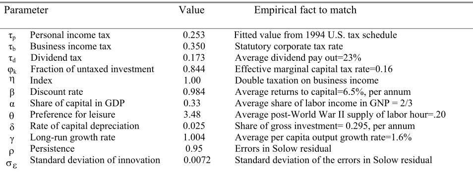
discount factor by setting the steady state interest equal to 6.5%, which is the average annual return to capital in the U.S.1 For our quarterly model we set β so that the quarterly interest rate is (0.065/4)%. In the neoclassical literature, the value of persistent parameter ranges between .9 and .979. We set ρ equal to .95. Following KR (1999) the standard deviation of innovation, σεis set

0.0072. KR chose the value of leisure preference parameter θ to match the steady state work hours, which is 0.20. Following them we set θ to be 3.48.

Personal income tax rate, τp, is set to 0.253, on the basis of the 1994 U.S. tax schedule for

married taxpayers with no children who file IRS form 1040 jointly. Corporate income tax rate, τb,

is set to 0.35, to match the statutory corporate tax rate. In the U.S. tax system, dividends received by a shareholder generally are taxed at the same rate that applies to the personal income tax; the capital gains, however, are taxed at a lower rate. The “Job and Growth Tax Relief Reconciliation Act of 2003”, reduces the 10- and 20-percent long-term capital gain taxes respectively to 5 and 15%. In our model, we do not specify the proportion of after-tax profit that is retained by the firm and that is distributed as dividends to the shareholders. As the dividend tax is generally higher than the tax on capital gains, if all the after-tax profit of the firm of our benchmark economy is taxed at the dividend tax rate, elimination of double taxation would generate an upward bias in our results. To avoid the bias, the after-tax profit of the firm is taxed at a rate equal to the weighted average of tax rates on retained earnings (capital gain) and tax rates on dividends. The average dividend pay out for all COMPUSTAT active firms for 1993-2003 was 17.62% and for 1983-1993 was 28.55%. The average retained earnings in these two periods respectively were 82.38% and 71.45%. Therefore, on average, in those 20 years the proportion of dividend paid out was 23% and the firms retained 77% of their after-tax profit. Based on these estimates, the tax rate on dividend (after-tax profit) for our benchmark model is calculated as follows: [average dividend pay out (23%)*tax rate on dividend (25%)+ average retained earning (77%)*capital gain tax rate (15%)]=17.3%.

To capture the double taxation of capital income the index η is set to 1. ϕ_k is set to 0.844 to match the effective marginal capital tax rate, which is 0.16.

Table 1: Parameter Values of Benchmark Model

Parameter Value Empirical fact to match

τp τb τd φk η β α θ δ γ ρ ε σ

Personal income tax Business income tax Dividend tax

Fraction of untaxed investment Index

Discount rate

Share of capital in GDP Preference for leisure Rate of capital depreciation Long-run growth rate Persistence

Standard deviation of innovation

0.253 0.350 0.173 0.844 1.00 0.984 0.33 3.48 0.025 1.004 0.95 0.0072

Fitted value from 1994 U.S. tax schedule Statutory corporate tax rate

Average dividend pay out=23% Effective marginal capital tax rate=0.16 Double taxation on business income Average returns to capital=6.5%, per annum Average share of labor income in GNP = 2/3 Average post-World War II supply of labor hour=.20 Share of gross investment= 0.295, per annum Average per capita output growth rate=1.6% Errors in Solow residual

Standard deviation of the errors in Solow residual

The long run growth rate of a neoclassical economy is determined by the exogenous rate of technological progress, γ. This long run rate remains unchanged in all the alternative tax policy regimes. Thus in the long run,

t y 1 t y t k 1 t k t c 1 t c ₊ = + = + = γ ,

Which is set to 1.004 in our model.

To analyze the short-run dynamics of the benchmark economy during different tax policy regimes, we linearize the first order conditions around the steady state as in King and Rebello (1988). The set of linearized equation yields the following law of motion for the state variables of our model:

1

1 +

+ = t + t

t ms

s ε .

The following equation specifies, given the initial capital stock and level of productivity, how consumption, work effort, investment, government expenditure, output and shadow prices are determined by the state variables, in response to a 1% negative productivity shock to the economy.

z_t =∏s_t,

4. Quantitative Results

We calculate the steady state value of output for our benchmark economy where individuals are taxed on their personal as well as corporate income and the firms are taxed on their profit. In period one, a negative and persistent shock hits the economy and drags output below its long run level temporarily. We solve the transitional dynamics of output, of the

benchmark economy, towards the steady state. In the next step, we assume a policy change in the economy that eliminates tax on dividend. The dynamics of output caused by this policy are solved and compared to the output dynamics in the benchmark economy. The difference between these two dynamics explains the effectiveness of the “end of double taxation” in stimulating the economy’s output level. We also evaluate the effectiveness of two other policies in reviving the economy from recession in the similar fashion. The first policy reduces the corporate income tax and the second policy reduces the tax on individual’s personal income. The impacts of the policies on the other variables of the economy, e.g. investment, employment, government

spending and welfare are also examined. Figures 1 through 10 plot the transition dynamics of the variables in alternative tax policy regimes. The quantitative results are presented in three

subsections. First, the impacts of permanent reforms in the tax policies are examined. Second, we solve the dynamics of the economy’s variables generated by temporary reforms in the policies. Third, the growth effects of both temporary and permanent policy reforms are briefly discussed.

4.1. Economic Recovery from the Permanent Reforms

The permanent tax policy reforms yield new steady state levels for the economy’s aggregates. The transitional dynamics from the original steady state levels to the new levels describes how the economy recovers from the recession with the help of alternative tax policies. The changes in the long run levels of the economy’s aggregates produced by the tax policies are reported in Table 2.

Table 2: Long Run Changes in the Levels

Tax Policy

Changes in Steady State Levels (in percentage) Output Investment Government Employment Welfare Spending

η=0

τb=0.27

τp=0.238

0.21 4.85

0.21 3.10 0.21 0.31

-8.89 -2.03 0.023

-5.26 -1.20 0.014 -3.92 0.16 0.009

Note: Row 1, 2 and 3 report the percentage changes in the steady state levels of the economy’s variables respectively generated by a permanent “end double taxation”, a permanent 8% reduction in the corporate income and a permanent 1.50% reduction in the personal income tax rate, compared to their steady state values in the benchmark economy with no reform. The percentage change in the steady state level of output

generated by a permanent “end of double taxation” is calculated using the following equation: _

    

 ₋

y y 1 y

,

where y is the steady state level of output in the benchmark economy with “double taxation” and y₁is the steady state level of output yielded by a permanent “end of double tax” policy.

As is clear, the level of output immediately shifts up following the “end of double taxation” and continues to move upward until it converges to its higher long run level. We calculate that the new steady state output produced by a permanent “end of double tax” policy is 0.21% higher compared to that in the benchmark economy.

In the next step, we examine whether the corporate or the personal income tax policy reforms can generate an equivalent increase in the long run output. Starting from the benchmark economy in which there is double taxation and the tax rates on personal and corporate incomes respectively are 25.3% and 35%, the tax on corporate income is varied. We find that a permanent 8% reduction in the corporate income tax yields a 0.21% increase in the long run output. From a similar exercise, we find that an equivalent increase in the long run output is produced when the personal income tax rate is permanently reduced to 23.8%. This rate is 1.2% lower than that in the benchmark economy. However, as dividend tax rate is calibrated as the weighted average of tax rates on dividend and capital gains and dividends are taxed at the same rate as the personal income, when the tax on personal income is reduced permanently, the tax on dividend is

essentially reduced permanently. This dividend tax rate is 17%, which is 0.3% lower than that in the benchmark economy.

Note: The dotted path describes the output dynamics in the benchmark economy. The ‘×’ path describes the output dynamics caused by a permanent “end double taxation”; the “•” path describes the dynamics generated by a permanent reform in the corporate tax and the‘◊’ path describes the dynamics generated by a permanent reform in the personal income tax policy.

income tax rate. In addition, the output trajectory in the “end of double tax” economy lies above those in the other economies for about 20 quarters.

A permanent “end of double taxation” also stimulates the economy’s long run investment level significantly. Figure 2A shows that this policy causes an immediate jump in the economy’s investment level; investment increases through time toward its new stationary level.

Note: The dotted path describes the output dynamics in the economy with “double taxation”. The ‘×’ path describes the output dynamics caused by a permanent “end double taxation”.

Investment dynamics produced by the alternative policy reforms are compared in Figure 2B. Although the corporate income tax policy reform initially exhibits an investment advantage over the “end of double tax” policy, the investment trajectory driven by the “end of double taxation” overtakes that driven by corporate tax policy reform approximately in one year and it eventually converges to a higher long run level.

In the long run, reductions in the corporate income or in the personal income tax that yield an equivalent “output effect” generate a relatively weak impact on the economy’s

Note: The dotted path describes the investment dynamics in the benchmark economy. The ‘×’ path describes the investment dynamics caused by a permanent “end double taxation”; the “•” path describes the dynamics generated by a permanent reform in the corporate tax and the‘◊’ path describes the dynamics generated by a permanent reform in the personal income tax policy.

The “end of double tax” policy produces a negative impact on the economy’s long run employment level. Figure 3A shows that the employment level drops immediately after imposition of this policy; it eventually converges to a new steady state level which is 2.03% lower than its benchmark level. It is to be noted that unemployment does not exist in our

Note: The dotted path describes the employment dynamics in the economy with “double taxation”. The ‘×’ path describes the employment dynamics caused by a permanent “end double taxation”.

A comparison of the employment dynamics produced by the alternative tax policy reforms are portrayed in Figure 3B. It appears that the economy’s long run employment is stimulated only when personal income tax is reduced. One possible explanation of this result hinges on the conflicting income and substitution effects of a change in the real wage. It follows from Equation (4) that a reduction in the personal income tax raises the real wage in the

economy. This encourages the individuals to work hard and produces a larger income effect. On the other hand, the “end of double tax” policy and a reduction in the corporate income tax induce the individuals to enjoy more leisure and produce larger substitution effects.

Note: The dotted path describes the government spending dynamics in the benchmark economy. The ‘×’ path describes the spending dynamics caused by a permanent “end double taxation”; the “•” path describes the dynamics generated by a permanent reform in the corporate tax and the‘◊’ path describes the dynamics generated by a permanent reform in the personal income tax policy.

government spending is significantly lower in the “end of double tax” regime compared to those in other policy regimes.

4.2. Economic Recovery from the Temporary Reforms

In this section, we assume that in the period immediately after the negative shock the government eliminates dividend taxes only for 12 quarters. In our set up, temporary reform in a tax policy is expected to have transitory impacts on the economy’s aggregates as the aggregates eventually converge to their original long run levels. Figures 5 through 8 plot the dynamics of the economy’s aggregates generated by temporary reforms in the tax policies.

The impacts of a temporary “end of double taxation” throughout the reform period are the same as those caused by the permanent “end of double tax” policy during the same span of time. For example, as Figure 5 shows, a temporary “end of double taxation” causes an immediate jump in output and the output trajectory lies above that in the benchmark economy throughout the reform period. We calculate that over these 12 quarters, the economy, on average, enjoys 0.38% higher level of output compared to the benchmark economy. But, immediately after the re-imposition of dividend tax, output drops by -1.81% relative to its benchmark level. After this massive decline, the output level increases slowly to catch up with its long run level.

While temporary reforms in the corporate tax and in the personal income tax policies stimulate the output level over the reform period, the impacts are much weaker than that generated by a temporary elimination of dividend tax. We find that over the reform period, on average, temporary reduction in the corporate tax or in the personal income tax, respectively yield a 0.056% and a 0.055% increase in the output level relative to that in the benchmark economy. While output exhibits a sharp drop immediately after the corporate or the personal income tax rates are raised back to their original rates, the magnitude of these drops are

considerably lower than that caused by the re-imposition of dividend tax. In addition, temporary reforms in the corporate or in the personal income tax policies cause a faster transition back to the steady state and also cause less loss of output relative to that caused by a temporary “end of double tax” policy during the transition towards the steady state.

Note: The dotted path describes the investment dynamics in the benchmark economy. The ‘×’ path describes the investment dynamics caused by a temporary “end double taxation”; the “•” path describes the dynamics generated by a temporary reform in the corporate tax and the‘◊’ path describes the dynamics generated by a temporary reform in the personal income tax policy.

transitional dynamics of investment generated by the temporary reforms in the tax policies. Termination of all the policy reforms after 12 quarters cause immediate decline in the economy’s investment level. However the magnitude of this downfall is greater for the re-imposition of dividend tax compared to those caused by the termination of other policy reforms. In addition, the investment trajectory generated by re-imposition of dividend tax lies below those generated by termination of the other policy reforms until it reaches the steady state. This implies that throughout the transition process, a temporary “end of double tax” policy causes greater loss of investment relative to that caused by the temporary reforms in the other tax policies.

Note: The dotted path describes the employment dynamics in the benchmark economy. The ‘×’ path describes the employment dynamics caused by a temporary “end double taxation”; the “•” path describes the dynamics generated by a temporary reform in the corporate tax and the‘◊’ path describes the dynamics generated by a temporary reform in the personal income tax policy.

Figure 7 shows that even during the reform periods a temporary “end of double taxation” or a temporary reduction in the corporate tax do not stimulate the economy’s employment level, which is consistent with the results for permanent policy reforms.

Note: The dotted path describes the spending dynamics in the benchmark economy. The ‘×’ path describes the spending dynamics caused by a temporary “end double taxation”; the “•” path describes the dynamics generated by a temporary reform in the corporate tax and the‘◊’ path describes the dynamics generated by a temporary reform in the personal income tax policy.

4.3. The “Growth Effects”

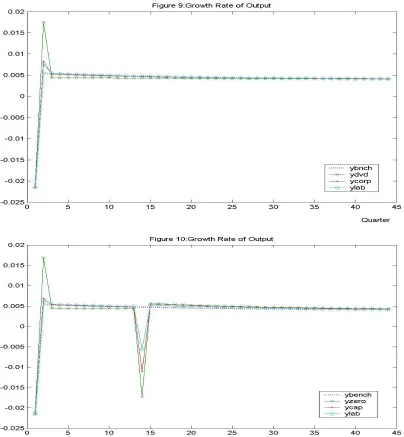
As the long run growth rate of our benchmark economy is determined exogenously, the tax policy reforms are expected to have only transitory effects on the economy’s growth rate. In this section, we analyze the effects of both “permanent” and “temporary” reforms in the tax policies on the short-run growth. The results are summarized in Figure 9 and 10.

Note: The dotted path describes the growth dynamics in the benchmark economy. The ‘×’ path describes the growth dynamics caused by the temporary “end double taxation”; the “•” path describes the dynamics generated by reform in the corporate tax and the‘◊’ path describes the dynamics generated by reform in the personal income tax policy.

The above results provide a few important messages regarding the impacts of the

alternative tax policies on the economy. For a quick economic recovery a temporary as well as a permanent reform in the policies appear to be useful. While the permanent reforms generate long run output advantages, the temporary reforms generate only temporary advantages. Therefore, the permanent reforms in the policies are preferable compared to the temporary reforms. While a permanent reduction in the corporate or in the personal income tax rate may yield the same “output effect” as that yielded by a permanent “end of double taxation”, initially the “end of double tax” policy exerts much stronger impact on output that lasts for a considerably long period (about 20 quarters). The permanent “end of double tax” policy also causes a faster transition back to the steady state output. The “investment effect” as well as the “welfare effect” of a permanent “end of double tax” policy appear to be stronger than those produced by the two other policy reforms. Thus as a tool for achieving quick economic recovery a permanent “end of double taxation” turns out to be more desirable than the two other policy reforms. On the other hand, when the reforms are adopted only for a short period, the transition period of output to its steady state is the longest for “end of double taxation”. In addition, the re-imposition of dividend tax causes greater output as well as investment losses compared to those caused by the

termination of two other policy reforms.

5. Sensitivity Analysis

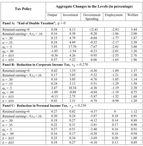
We perform some computational experiments with different choices for some parameter values to determine the robustness of the main quantitative results derived in the previous section. Table 3 reports the results of these experiments.

First two rows of Panel A in Table 3 reports the steady state impacts of a permanent “end of double tax” policy in an economy that departs from the benchmark economy only with respect to the firm’s decision regarding dividend pay out. In the pervious section, we used a tax rate of 17.3% on dividend based on the historic average of 77% earning retention rate of the firms. In this section, we re-calculate the impacts of the tax policies by changing the proportion of after-tax profit retained by the firms. First, we assume that the firms do not retain any earnings after paying tax on its profit. Hence, given that the “double taxation” prevails in the economy, the shareholders pay tax on their dividends at the rate that applies to personal income.

Table 3: Sensitivity Analysis

Note: In our benchmark economy, the share of capital in output, α=0.33, the fraction of deductible business taxable income, ϕk = 0.844, the capital depreciation rate, δ= 0.025, the double taxation index, η=1, the corporate income tax

rate, τb=0.35 and the personal income tax rate, τp=0.253.

The tax function takes the following form:

) i k r ( )] i k r )( 1 ( n w [

t_t =τ_{p t t} +η −τ_{b t t} −φ_{k t} +τ_{b t t} −φ_{k t} (15)

We find that when the firms distribute the entire after-tax profit as dividends, a permanent “end of double tax” policy exerts much stronger long run impacts on output as well as on

Aggregate Changes in the Levels (in percentage) Tax Policy

Output Investment Government Spending

Employment Welfare

Panel A: “End of Double Taxation”, η =0

Retained earning=0 0.58 8.13 -12.43 -2.93 3.44

Retained earning=. 9,τd = .16 0.16 4.38 -8.20 -1.86 2.08

α = .30 0.15 4.79 -8.04 -1.77 1.87

α = .35 0.24 4.89 -9.32 -2.17 2.58

ϕk = .5 3.93 17.70 -7.67 -2.01 3.88

ϕk = .99 -1.85 -1.54 -8.33 -2.01 1.26

δ = .015 -0.36 4.26 -9.95 -2.55 2.76

δ = .035 0.57 5.22 -8.06 -1.65 1.96

Panel B: Reduction in Corporate Income Tax, τ_b =0.270

Retained earning=0 0.42 3.55 -4.56 -1.09 1.37

Retained earning=. 9,τd =.16 0.17 3.03 -5.32 -1.21 1.38

α = .30 0.16 3.05 -4.76 -1.05 1.14

α = .35 0.24 3.13 -5.51 -1.29 1.58

ϕk = .5 2.47 10.34 -4.36 -1.19 2.38

ϕk = .99 -1.09 -0.89 -4.94 -1.19 0.75

δ = .015 -0.13 2.75 -5.87 -1.52 1.68

δ = .035 0.42 3.31 -4.78 -0.98 1.20

Panel C: Reduction in Personal Income Tax, τ_p =0.238

Retained earning=0 0.27 0.82 -4.37 0 1.12

Retained earning=. 9,τd =.16 0.20 0.24 -3.87 0.18 0.91

α = .30 0.18 0.27 -4.12 0.14 0.88

α = .35 0.22 0.31 -3.81 0.17 0.98

ϕk = .5 0.27 0.51 -3.40 0.16 0.92

ϕk = .99 0.16 0.17 -4.30 0.16 0.94

δ = .015 0.25 0.34 -3.69 0.20 1.00

investment than those in our original exercise. These long run impacts are also significantly greater than those produced by the other policy reforms. On the other hand, when the earning retention rate is high (90%), the impact of “end of double tax” policy on the long run output is a little weaker than those caused by the other policy reforms. The intuition of these results can be understood by comparing Equation (4) with Equation (15). It follows from Equation (4) that when the firms retain a proportion of after-tax earning, the shareholders pay tax on the dividends at a rate of τd, which is calibrated as 17.3%. On the other hand, Equation (15) shows that when

the firms distribute the entire after-tax profits as dividends and “double taxation” prevails, dividends are taxed at a higher rate (25.3%). Therefore when the dividend pay out ratio is high and the tax on dividend is eliminated, the shareholders receive higher returns on their investment compared to that when the dividend pay out is less. This encourages the shareholders to invest more.

We test the sensitivity of our results to capital’s share in total output by considering an increase in capital’s share (set α= .35) and also a decrease in capital’s share (set α= .30) in output relative to that in the benchmark economy. For a higher value of α, the impact of “end of double taxation” is stronger than that for its benchmark value; for a lower value, its impact appears to be considerable. In addition, for both values of α, the impact of this policy on the long run investment is significant. These results prove the robustness of our previous findings.

6. Conclusion

The paper evaluates the effectiveness of “end of double tax” policy in stimulating a quick economic recovery. We compare the impacts of this policy with those of two other policy

reforms that reduce personal income and business income taxes. We consider both “permanent” and “temporary’ reforms in these policies. A simple neoclassical model with exogenous growth is used as a benchmark economy.

We find that the tax policy reforms have considerable influence on the economy and that the transitional effects of different policy reforms on the economy’s variables play a useful role in evaluating the overall impact of the policies. Given that the temporary reforms only offer temporary benefits, the permanent reforms in the taxation policies are more useful for the long run economic well-being. While all the tax policy reforms considered in this study stimulate the long-run levels of output as well as investment of the economy, we find a significant quantitative difference. A permanent “end of double taxation” yields higher level of output compared to those yielded by permanent reforms in the other policies for a considerably long period; this policy also causes a faster transition back to the steady state output. The reforms in the corporate income or the personal income tax policies that yield an equivalent steady state “output effect” generate a relatively weak impact on the economy’s long run investment level. A sensitivity analysis performed in section 6 proves the robustness of our analysis and also gives us some additional insights regarding the effectiveness of the “end of double tax”. We find that eliminating dividend tax can actually reduce the steady state output if the firm’s investment expenditure is almost entirely deducted from their taxable income. On the other hand, when the firms are taxed on a significant proportion of their investment spending, eliminating dividend tax exerts significant output benefit. We also find that the higher is the dividend pay out, the greater is the impact of “end of double tax” policy on the long run output of the economy. Based on our findings we claim that a permanent “end of double taxation” is an effective fiscal tool for stimulating an economic recovery.

Essay 2: Prospect Theory and the Welfare Cost of Business Cycles

1. Introduction

According to Lucas (1987), the welfare cost of business cycles is small and negligible. Using a simple representative agent model where preferences of the agents are logarithmic, he estimates the welfare cost as the percentage of consumption the consumers would be willing to pay to switch from a fluctuating consumption path to a perfectly smooth consumption path. He finds that to have all the volatilities in consumption eliminated, the consumer would only give up less than one-tenth of one percent of consumption (about $8.5 per person per quarter).

Lucas’s provocative claim naturally stirs up a series of new attempts to re-examine the issue. Many of these efforts involve the relaxation of Lucas’ assumptions on consumer

preferences and the consumption processes. In a later survey paper, however, Lucas (2003) points out that these extensions mostly give rise to similar conclusions. For example, Otrok (2001) incorporates time-non-separabilities in consumer preferences in his welfare cost

calculation, and finds that the welfare cost is of the same magnitude as that estimated by Lucas. Dolmas (1998) estimates the potential welfare gains from eliminating consumption volatility using non-expected utility and finds that depending on parameter choices, the gains range from one to twenty percent of consumption. However, he concludes that for reasonable parameter choices the welfare cost of consumption volatility is always significantly below the welfare benefit of an additional percentage point of consumption growth in perpetuity. Campbell and Cochrane (1999) calculate the welfare cost by incorporating habit formation into the formulation of consumer preferences. They find that the cost of consumption volatility is significantly large. However, Lucas points out that the result largely hinges on the relaxation of the size of an extra parameter that does not exist in standard utility functions.

affected by the gains and losses in their wealth and not by the final state of their wealth. Second, when the agents experience an equal amount of gain and loss in their wealth, they are hurt significantly more by the loss than get pleasure from the gain. This attitude of the agents is termed as “loss aversion.” We believe these behavioral rules may turn out to be crucial in terms of measuring the cost of business cycles. For one thing, we concern about business cycles mainly because of the possible losses – either losses of consumption during a recession, or losses of wealth during inflation. For another, most would not deny that these losses concern us more than the gains during “good times.”

The prospect theory has been quite popular in economics and behavioral finance. In particular, it has been used to offer a solution for the “equity premium puzzle” in financial market studies. The equity premium puzzle refers to the abnormally high difference in the returns between a risky asset such as equity and a risk-free asset that cannot be explained by theories. Benartzi and Thaler (1995) argue that if an investor is loss averse and has the tendency to monitor changes in the value of his portfolio frequently, a high equity premium is required to compensate him for the volatilities in stock returns. Barberis, Huang, and Santos (2001) offer an explanation of the equity premium puzzle using the prospect theory preferences in a general equilibrium framework. They show that if the loss aversion attitude of an investor is combined with the tendency to become more risk-seeking after gains have occurred and more risk-averse after a sequence of losses, highly volatile stock returns and high equity premium might be generated in equilibrium.

investments to switch from the world with return fluctuations to the world of zero fluctuations. We believe that this indicates a welfare cost that is much larger than Lucas’s estimates.

Our study therefore relies heavily on the premises of the prospect theory that losses in financial returns are critical to consumers, and such losses occur during the course of business cycles and can be used to measure the cost of these cycles. A natural question, then, is how closely fluctuations in investment returns are related to business cycle fluctuations. Researchers have documented substantial linkages between an economy’s performance and the performance of financial markets, including the procyclical movements of stock prices. In fact, the positive correlation of stock price index and real economic activity over the course of many business cycles is one of the major empirical facts about the US economy. If the macroeconomic growth rises, demand for a typical company’s product rises and the revenue of the company should also increase. This leads to an appreciation of the company’s share price. Likewise, during a

marcoeconomic downfall the demand for a company’s product declines and this eventually results in a share price decline.

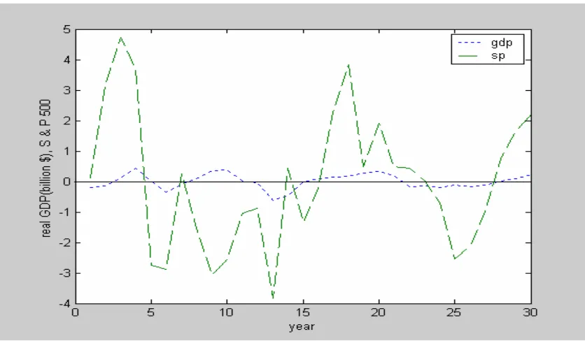
Figure 11: Real GDP and S & P 500 Composite Index

In Figure 11, we plot HP-filtered real GDP of the U.S. and the S&P 500 stock index. It is quite evident that, while the stock price index is much more volatile than GDP, it is strongly pro-cyclical. We calculate the contemporaneous correlation between the real GDP and stock price as 0.37. Our findings resemble the time series analysis of the major macro variables documented by King and Rebelo (2000).

Financial returns and business cycles are related in another important aspect. The stock market is forward-looking and responds to where the economy is going in the near future. If the economy is currently in a recession, the stock market will predict a recovery before it actually takes place and the stock price will rise before the recession ends. Pearce (1983) evidences that, with a very few exceptions, stock price movements have been a valuable leading indicator of the business cycles in the US economy. The traditional view as to why movements in stock prices generally precede the movements in real economic activity suggests that stock prices equal the present value of a company's expected future profits. If the investors lower their expectation of profits because of a prospective economic downturn, stock prices would fall immediately, i.e. before the actual fall in the company’s profit and economic activity. Another view of why stock prices may lead economic activity emphasizes investors' level of confidence about the economy. If investors are optimistic about the prospect of the economy, they would be willing to make investments and the stock prices would begin to rise. On the other hand, pessimism about the economy will drag stock prices down.

The rest of the paper is organized as follows. Section 2 offers a brief review of prospect theory preferences. Section 3 discusses the framework of our analysis and also outlines the methodology used to estimate the welfare cost. Section 4 presents the results. Section 5 tests the robustness of the results. Section 6 concludes the paper.

2. The Prospect Theory and Consumer Preferences

loss function is steeper than the slope of the gain function, implying that the agent weighs the disutility from a loss more strongly than the utility from the same magnitude of a gain. The ratio of the slopes at the origin is a measure of loss aversion. Kahneman and Tversky (1979) propose the following prospect utility function:

   

< −

−

≥ =

0 ,

) (

0 ,

) (

X if X

X if X X

v _β

α

λ , (1)

Where X is a change measured as the difference in wealth relative to the benchmark level of wealth. While Kahneman and Tversky use previous period’s wealth level as the benchmark, both the purchase price the investor pays for her wealth and the returns on wealth in the previous period are also reasonable benchmark levels of wealth. WhenX ≥0, the agent’s wealth level is higher than the benchmark, a gain is realized. According to equation (1), this yields utility from the gain in her wealth level. Otherwise, when X<0, the agent’s wealth level is lower than that at the benchmark level – a loss has occurred. As the agent is more sensitive to a loss realization, her level of disutility from a loss is higher than the utility from a gain by the degree of loss aversion

λ, which is set to be larger than 1. The parameters αand β are estimated to be 0.88.

Figure 12: Utility Function Supported by the Prospect Theory

Figure 12 displays the form of the prospect theory preferences. When the agent realizes the same amount of gain and loss is her wealth level, the disutility caused by the loss, AC is larger than the utility caused by the same amount of gain, AB.

3. The Framework

The framework of this paper is a simplified version of Barberis, Huang, and Santos (2001)’s consumption-based asset pricing model2. The agents of the economy invest in assets each period. There are two types of assets in the economy: a risky asset and a risk-free asset. Consumer preferences bear the same feature as the one presented in the previous section.

3.1. Consumer Preferences

The representative agent derives utility from the returns on her investments as well as from consumption. The preferences of the representative agent are of the following form:

max         + − ∑ ∞ = − 0 1 )) ( 1 ( t t t t t

t C _{b v X}

E ρ

δ

ρ δ (2)

Where the parameter 0<ρ<1 is the time discount factor and δ >0 controls the curvature of utility over consumption. The first term of the utility function represents the utility over consumption at period t. The second term of the utility function represents the agent’s utility from the returns on her investments. The variable Xt represents the returns the investor realizes at period t from her

investments at period (t-1). The utility she receives from Xt is given by the function v. This

implies that the agent cares about the returns on her investments and derives direct utility from the returns. The parameter, bt is the exogenously determined scaling factor that captures the

overall importance of utility from fluctuations in the returns relative to the utility from

consumption. bt is specified as follows:

γ

−

= t t b C

b ₀ , where C_t is the aggregate consumption at

period t. We assume that b0>0, as b0 = 0 reduces our framework to the consumption-based model

with power utility.

2 _{Barberis, Huang, and Santos assume that the degree of loss aversion depends on the prior investment performance.}

3.2. Measuring gains and losses

We consider the returns on the risk-free asset offered by the economy as the benchmark to which the agent compares gains and losses from her investments in the risky asset. In the beginning of each period the agent decides to invest in the risky asset. At the end of each period the agent compares the returns she receives from the risky assets to the risk-free rate offered by the economy in that period. The difference between the risky and the risk-free returns is referred to as the “excess return.” If in any period the excess returns turn out to be positive the agent has realized a gain on her investments in that period, while the negative excess returns imply that a loss has occurred. Specifically, if R_tis the return on the risky asset received by the agent at the

end of period t-1, i.e. at period t and R_ftis the risk-free rate offered by the economy at period t,

then, at the end of period t-1, the agent realizes a gain if:

t f t

t R R

X = − >0 and a loss: if

t f t

t R R

X = − <0.

The logic behind such a definition of gain or loss is that, the investor is likely to be disappointed with her decision to invest in the risky asset when the returns she receives from the risky asset is less than the risk-free rate offered by the economy. For example, if in any period the risk-free rate is 4% while the agent receives 3% from investing in the risky asset, she might regret her past decision to invest in the risky asset as she could have avoided the risk associated with the risky investments and realize higher returns by deciding to invest in the risk-free asset. On the other hand, when the returns on risky investments is higher than that from the risk-free asset the investor is likely to be happy about her decision of investing in the risky asset and consider the positive excess returns as a gain from her investments. This is a key feature of the prospect theory.

3.3. Utility from Gains and Losses

To define the investor’s utility from returns, we consider two separate cases. First, we consider a linear prospective function where the utility from returns depends only on the

investor’s degree of loss aversion. This is captured by the following prospective utility function:

   < ≥ = 0 , 0 , ) ( X if X X if X X v t t

This is a linear prospective utility function similar to that displayed in Figure 12. λ=1 corresponds to loss neutrality and loss aversion grows as λ increases. Thus the function allows us to investigate whether the agent’s perception about the fluctuations in the returns changes when her degree of loss aversion changes.

Our second prospective preference is the same as that proposed by Kahneman and Tversky, Equation (1). The function is similar to that shown in Figure 12, however, is slightly concave over gains and convex over losses.

3.4. Welfare Cost Estimation

We calculate the welfare cost of business cycles using Lucas’s method. Lucas’s method of welfare cost estimation is simple. He specifies a preference function for the representative consumer and a consumption process that resembles the actual aggregate consumption time series of the US economy. The expected utility the consumer receives from the fluctuating consumption stream is compared to the utility the consumer receives from the smooth consumption stream with the same average consumption growth rate. The welfare cost is the percent of consumption the consumer would pay, at every date and state, to switch from the fluctuating economy to the non-fluctuating economy. Specifically, Lucas calculates the percent of consumption, g, which satisfies the following:

∑

∑

0[ (1 ) ] [ ( )]

t s t t t t

t_{U g c E U c}

E ρ ρ (4)

The left-hand side represents expected utility the agent derives from the fluctuating consumption stream, 0

t

c and the right hand side is her expected utility from the smooth consumption

process s t

c . “g” is the percent of consumption the consumer would pay to move from the fluctuating consumption stream to the smooth consumption stream. According to Lucas’s definition, “g” represents the welfare cost of business cycles to the consumer. Using a constant relative risk aversion (CRRA) preference function and a consumption stream that includes a trend and also a cycle component, Lucas calculates “g” as follows:

2 z 2 z . 2 1 ) (

g σ ≅ σσ (5)

The complexity of our utility function in (2) makes this calculation less straightforward. However, a useful simplification makes this function more tractable. Note that the first part of our utility function is essentially identical to Lucas’s. Since he already concludes that the welfare cost of this part is negligible, we can ignore gains and losses resulted from it by setting c to be a constant for all t. Moreover, this also allows us to isolate the effect of loss aversion on the welfare cost of business cycles. Thus, we focus on the cost of fluctuations in the asset returns.

We need to define our new variables for the left-hand-side and the right-hand-side for (4). “Smooth returns” refer to the average excess returns the agent receives from her long-term investments in the risky asset. We put this on the right-hand-side. “Fluctuating returns” refers to the excess returns the agent receives each period from her investments in the risky asset. We put in on the left-hand-side. The "prospective utility" the agent receives from the fluctuating returns is computed by taking the expected value of utilities from gains and losses realized by the agent each year. Expected prospective utility the agent receives from the fluctuating returns is

compared to her utility over the smooth returns. The welfare cost of the fluctuating returns is the percent of the average excess returns the investor would give up at every period, to move from the world of the fluctuating returns to the world of smooth returns.

or,

∑

∑

= = = − n t t t t t t n t

t_{U E X g E U X}

0 0 )] ( [ ] ) ( [ ρ

ρ , (6)

Where n is the number of periods considered in this study. “g” is the percent of the excess returns required to leave the agent indifferent between the world of fluctuating returns and the world of smooth returns.

We assume that the agent’s expectations about the excess returns remain unchanged over the years, e.g. E_t =E. LetE_t(X_t)= X. As X is positive, Equation (6) can be written as

follows: ) X ( EU ) g X ( _t n 0 t

t _{− =}

ρ

∑

= (7)

From Equation (7), the welfare cost of volatility is calculated as follows:

)] X ( EU ) 1 1 [( X g _t n ρ − ρ − −

= (8)

) X ( EU ) g X ( _t n 0 t

t _{− =}

ρ α

∑

= (9)

From Equation (9), the welfare cost of volatility is calculated as follows:

α ρ − ρ − − = 1 t n)EU(X )] 1

1 [( X

g (10)

We estimate “g”, by substituting U(Xt) in the right-hand side of Equation (8) and (10) by

the appropriate prospective utility function for gains and losses realized by the investor each year.

Our assumptions about a constant long-term expected return and fluctuating annual returns map closely into the stylized facts of the financial market. In the time series, the annual returns on a typical risky asset such as stock has a high mean and excessive volatility, whereas the annual returns on a risk-free asset such as Treasury bills has a lower mean and very modest volatility. In the cross section there is a substantial premium, i.e., the average difference between the returns on a typical stock and Treasury bills is historically positive and very large.3

Therefore, in any specific year, the returns on investments in the risky assets are uncertain, but it is certain that the investor will realize a substantial gain from her long-term investments in the risky asset. The positive average excess returns the investor receives from her long-term

investments deliver positive utility. On the other hand, as the annual returns on the risky asset are volatile, the annual excess returns over the risk-free returns are also volatile. In some periods the excess return is positive, causing gains and delivering utility to the agent, while it is negative in other periods, causing losses and delivering disutility to the agent.

4. Computation and Quantitative Results

We need to calibrate two key parameters for calculating the welfare cost. The value of λ

determines how keenly an agent feels a loss relative to a gain. The higher the value of λ, the higher the degree of loss aversion of the investor, and her utility level will decline more rapidly when a loss occurs. Tversky and Kahneman (1992)’s estimate suggest that the disutility of a loss is twice as much as the utility of a gain of the same magnitude. They estimate λ=2.25. We use

3 _{Mehra (2003) reports that over the last century the average annual returns on the U.S. stock market has been 7.8%}

different values in the neighborhood of 2. In the standard literature the value of the parameter determining the curvature of the utility function usually ranges between 0 and 3. We assign different values of α that ranges between 0.05 and 3.

We calculate the value of g by using the financial market data. The annual returns on the S & P 500 index are obtained for the years 1962-2002 from the CRSP database to represent the returns on the risky asset. The returns on Treasury bills are obtained from the Federal Reserve Bank of St. Louis’s database for the same sample period. For our sample period, the average annual return on the S & P 500 is high (11.89%) and it is volatile with a standard deviation of 16.63%. The average annual return on Treasury bills is 5.97% with a standard deviation of 2.52%.

In the first step of the welfare cost estimation, we calculate the annual outcome of the agent’s investments in the risky asset by comparing the annual returns on the S & P 500 to those from the Treasury bills. It is to be noted that we do not distinguish between the total value of the investor’s holding of financial assets and the total value of financial asset she invests in the risky asset. Although there are two types of assets in the economy, we assume that the agent invests only in the risky asset and uses the returns on risk-free asset as a benchmark to evaluate the gains and losses on her investments. When the risk-free returns of the economy is considered as a benchmark, it is irrelevant whether gains and losses from investments are calculated over the total financial wealth of the agent or only over her total investments in the risky asset. The reason is as follows: if B and S represent the agent’s holdings of the risk-free asset and the risky asset, and she considers the risk-free rate as the benchmark, then at time t, the returns on investment = (BR_ft+SR_t)-(B+S) R_ft is the same as S(R_t −R_ft). Assuming that each year the agent invests $1

from the fluctuating returns to the expected utility she derives from the smooth returns to calculate the cost of fluctuating returns.

We calculate the costs of fluctuating returns for different values of loss aversion parameter using Equations (8) and (10). We also calculate the costs by substituting the

consumption volatility,σ_z, in Equation (5) with the returns volatility, i.e., we set σ_zto 0.1670, which is the standard deviation of excess returns. The costs calculated from Equations (8) & (10) and Equation (5) allow us to compare the costs of volatility produced by prospective preference with those produced by Lucas’s preference. Table 4 summarizes the results. The entries in the table are the percentage of the excess returns the investor is willing to give up to switch to a world of smooth returns from a world of volatile returns.

Table 4: Welfare Cost of Fluctuations in Asset Returns

Lucas

(return) λ =1 λ =1.5 λ =1.8 λ =2 λ =2.25 λ =2.5 λ =3

α= 1 1.39 0.28 2.58 3.97 4.89 6.04 7.19 9.49

α=. 05 .069 5.92 5.92 5.92 5.92 5.92 5.92 5.92

α=. 1 0.14 5.91 5.92 5.92 5.92 5.92 5.92 5.92

α=. 2 0.28 5.85 5.91 5.92 5.92 5.92 5.92 5.94

α=. 5 0.70 3.98 5.25 5.69 5.86 5.91 5.81 5.10 Note: The values of α represents the degree of risk aversion for Lucas preference. α=1 reduces the

Kahneman and Tversky utility function to a linear prospective utility function.

The welfare cost of fluctuating returns for prospective preference ranges from 2.58-9.49% of the average excess returns. In dollar terms, if in any year the investor receives 11.89% returns on the dollar she invested in the S & P 500 and the returns on Treasury bills in that year is 5.97%, she would be willing to pay $0.15 [(11.89-5.97)*2.58%]-$0.56[(11.89-5.97)*9.49%] to have all the fluctuations associated with the returns on the S & P 500 eliminated.

consumption4. The effect of loss aversion on the welfare costs of business cycles are revealed when we compare the costs produced by the prospective preference with those reported in column 2. The first row reports the costs associated with the linear prospective function. The results give two important insights regarding the impact of loss aversion on the welfare costs of volatility. First, expect for the case of loss neutrality, costs associated with the prospective utility are higher than those with Lucas preference. Second, as the degree of loss aversion grows, the welfare costs increases. These results suggest that while higher volatility in asset returns generates higher welfare costs, inclusion of loss aversion into the agents’ preferences also contributes to the higher welfare costs.

Rows (2)-(5) reports the costs calculated from Equation (10). As for the linear prospective preference, the welfare costs produced by the Kahneman and Tversky utility are significantly larger than those produced by Lucas’s preference. By comparing the costs produced by Kahneman and Tversky utility for loss neutrality (λ =1)with those reported in Column 2, it is confirmed that the specific form of the preference function also generates higher welfare costs. Our findings, therefore, suggest that both aspects of the prospect theory: the investors care about their asset returns and that they are loss averse generate higher welfare costs. However, it is also to be noted that, while inclusion of loss aversion contributes to the higher welfare costs,

estimates in rows 2, 3 and 5 imply that the costs do not necessarily increase with higher λ. This implies that while the investor has loss aversion attitude, the degree of loss aversion is limited.

5. Sensitivity Analysis

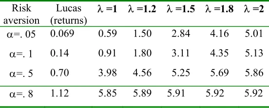
The welfare costs estimated for different values of risk aversion and loss aversion parameters in the previous section are large. In this section, we analyze whether these estimates change with alternative specification of prospective preferences and a different data set.

We consider an exponential prospective preference function where the utility of the investor depends on the degrees of both risk aversion and loss aversion. This is captured in the following utility function:

4 _{The standard deviation of the log of US real quarterly consumption reported in Lucas (1987) is 0.013. We find that}