Vol. 3, No. 1, (2013), 13-30
A level set moving mesh method in
static form for one dimensional PDEs
Maryam Arab Ameri
Abstract
In this paper, we propose an adaptive mesh approach for time dependent parial differential equations, based on a so-called moving mesh PDE(MMPDE) and level set method. It means that the velocity of mesh nodes is calculated by MMPDE and is employed as veocity in the level set equation. Then, at each time level, the mesh points are considered as the level contours of the level set function. Finally the method is merged with local time step technique.
Keywords: Adaptive grid; Level set function; Level contours; Moving mesh; Local time stepping refinement; MMPDE.
1 Introduction
In this paper, we discuss a class of adaptive mesh algorithms for solving time-dependent partial differential equations(PDEs) whose solutions have large variations over a given physical domain, such as shock waves, boundary layer and interior layer.
This method is based on the level set concept. the level set methods are powerful numerical techniques for tracking the evolution of interfaces moving in complex ways. The level set methods were used for the first time to repre-sent the evolution of surfaces implicity by Osher and Sethian [11]. Due to its many advantages, this approach has been used for many cases [1, 5, 9, 13, 19], for example, it has been used for mesh generation around a body(inside or outside) by the level set function [12]. Liao et al. presented some points about using the level set functions for moving grid based on deformation method [6]. In this paper, we also formulate an adaptive mesh method which is based on the level set method. This method is combined with a class of moving mesh methods which employs a moving mesh partial differential equation, MMPDE, to perform mesh adaptation. The MMPDE is formulated in terms of coordinate transformation or mapping,[3, 4, 8, 16, 17]. Several moving mesh equations(MMPDEs) based upon equidistribution principle have been
Maryam Arab Ameri
Department of Mathematics, University of Sistan and Baluchestan, Zahedan, Iran. e-mail: [email protected]
derived in [3], where in Section 2, we briefly review some of them. Finally after introducing the new method, we present local time stepping refinement technique based on the slope of the level set function for increasing the effi-ciency of the moving mesh method. The mentioned method is used to solve scalar field satisfying
ut(x, t) =L(u), (1)
where L is a differential operator defined on physical domainΩ,a≤x≤b
and 0≤t≤Tf.
2 Moving Mesh Methods
In this section, we develop a new moving mesh method based on the level set concept. We start with a review of the equidistribution principle(EP)[3, 15] and derive MMPDEs from that principle in subsection 2.1,then a description of adaptive grid based on level set method is given in the subsection 2.2.
2.1 MMPDE
The evolution of moving computational grid can be viewed as a discretiza-tion of a one-to-one time dependent coordinate mapping. Letxandξdenote the physical and computational coordinates, with domainsΩandΩc, respec-tively. Without loss of generality, both of them are assumed to be in [0,1]. Define a coordinate transformation by:
x=x(ξ, t), ξ∈[0,1], x(0, t) = 0, x(1, t) = 1. (2)
The computational coordinates is discretized on a uniform mesh given by
ξj= j
N, j= 0,1,· · ·, N,
whereNis a certain positive integer and the corresponding mesh inxdenoted by
0 =x0< x1(t)< x2(t)<· · ·< xN−1(t)< xN = 1.
A major factor of moving mesh approach is the monitor function, ρ(x, t), which is chosen to be somehow a measure of the solution error. For a given monitor function, the mesh point locations,xj(t), could be required to satisfy the following equidistribution principle (EP) for all the values of timet[3]:
xj(t)
xj−1(t)
ρ(x, t)dx= 1
N
1
0 ρ
(x, t)dx= 1
or equivalently xj(t)
0 ρ(x, t)dx=
j
Nθ(t) =ξjθ(t). (3)
By differentiating (3) with respect to ξ once and twice,, we obtain two dif-ferential forms of EP,
ρ(x(ξ, t))∂
∂ξx(ξ, t) =θ(t), (4)
∂
∂ξ(ρ(x(ξ, t), t) ∂
∂ξx(ξ, t)) = 0. (5)
These EPs,(3),(4) and (5), which do not contain the node speed ˙x(ξ, t),are called quasi-static EPs(QSEPs). Related to these QSEPs, various MMPDEs were derived in [3] by taking the mesh to satisfy the above EP (Eq. (5)) at a later timet+τ instead of att. In this case the mesh should satisfy
∂
∂ξρ(x(ξ, t+τ), t+τ) ∂
∂ξx(ξ, t+τ) = 0 (6)
where the parameter τ is called a relaxation time. By expanding the term ∂
∂ξx(ξ, t+τ) in Taylor series and dropping certain higher order terms, various MMPDEs can be obtained. Two of them which are used in our work are MMPDE5 and MMPDE6:
M M P DE5 : −x˙ =−1
τ ∂ ∂ξ(ρ
∂x
∂ξ), (7)
M M P DE6 : ∂
2x˙
∂ξ2 =−
1
τ ∂ ∂ξ(ρ
∂x
∂ξ). (8)
These MMPDEs and also the rest of them not only force the mesh ,x(ξ, t), toward equidistribution principle but also prevent the mesh from crossing. More specifically, the term −(1τ)(∂ξ∂(ρ∂∂ξx)) plays the fundamental role of a correction term to make the mesh equidistribute the monitor function and it is stabilizing term for the mesh trajectories.
The monitor function,ρ, is chosen such that the mesh points are concentrated in regions where more accuracy is needed, and so ρ is usually taken to be some measure of the solution error estimated from discrete solution values. A commonly used monitor function isρ=1 +αu2x (αis regularizing factor), which equidistributes the arclength of the solution u.
In this work, we discretize MMPDE5 and MMPDE6 by centered finite dif-ference in space, which yields for MMPDE5
˙
xj =Ej
τ , j= 0,1, . . . , N
˙
xj+1−2 ˙xj+ ˙xj−1=−Ej
τ , j= 0,1, . . . , N.
The quantityEjrepresents a centered approximation to the term on the right hand side of MMPDE5 and MMPDE6 given by
Ej=Mj+1/2(xj+1−xj)−Mj−1/2(xj−xj−1), j= 0,1, . . . , N
where Mj+1/2 = 21(Mj+Mj+1), Mj = M(uj), and uj ≈ u(xj, t) is an ap-proximation of the solution at grid pointxj.
2.2 Moving Mesh Based on Level Set Approach
In this section, at first a new moving grid method is formulated, and then the algorithm of this method is presented.
Essential point in all applications of the level set method is using the implicit representation. This point is also used in grid generation in such a way that the mesh nodes are represented implicitly by the level contours of the level set function. In this method, at each time level we construct the level set function,ψ(x, t), and the mesh pointsxj, j= 0,1, . . . , N, are obtained by the level contours of ψ(x, t), that means the mesh points are:
{xj |ψ(x, t) =cj, j= 1,2, . . . , N} (9)
wherecj isj-th component of a constant vectorC= (0,N1,N2, . . . ,1) andN is the number of mesh points.
In fact, in each time, we seek a level set function, ξ = ψ(x, t) : Ω → Ωc , which maps xj to cj = Nj, j = 0,1, . . . , N and satisfies the well-known equidistribution principle
Jρ=|Ωσ
c|, (10)
where J is the Jacobian of the coordinate transformation x = ψ−1(ξ, t) :
Ωc → Ω, and ρ = ρ(x, t) is a given monitor function, and σ = σ(t) =
Ωρ(x, t)dx.
For updating the level set function or equivalently for updating the position of mesh nodes, the well-known level set equation is applied,
ψt(x, t) +vψx(x, t) = 0. (11)
ψ(0, t) = 0, ψ(1, t) = 1.
As we mentioned at each time level, any
ψ(x, t) =a (12)
has a correspondence point on x-axis which is one of the new mesh nodes. By differentiating (12) with respect tot, we get
ψt(x, t) +ψx(x, t) ˙x= 0, (13)
and when compared with (11) and (13), we get
˙
x=v, (14)
that means, the nodes velocity is equal tov.
So for calculating the nodes velocity in the level set equation, the MMPDE5 or MMPDE6 should be applied which generates an equidistributed mesh through this algorithm.
At each time level, after determining new nodes, the solution of PDE should be determined. For this purpose, let
˜
U(ψ(x, t), t) =u(x, t), (15)
then
˜
Ut=uxx˙+ut
where ut=L(u) by (1) and ˙x=v by (14). The derivatives in L(u), such as
ux, uxx are also transformed. For example, from (15), we have
˜
Uψ=uxxψ ⇒ux= ˜
Uψ
xψ = ˜
Uψ σ ρ|Ωc|
=ρ|Ωc|
σ U˜ψ,
˜
Uψψ =uxx(xψ)2+uxxψψ⇒uxx= ˜
Uψψ−uxxψψ (xψ)2 = (
ρ|Ωc|
σ )
2( ˜U
ψψ−uxxψψ).
The higher derivatives can be derived similarly. The transformed equation for ˜U(ψ, t) takes the form of
˜
Ut= ˜L( ˜U), (16)
2.3 Algorithm of Adaptive Level Set Method(ALSM)
In this section, we provide an algorithm to solve the given PDE (1) in a moving grid based on the level set function.
Step1:Enter the initial time, t0, the final time,Tf, the length of time step,
Δt, and the number of mesh points,N.
Step2:Seti= 0.
Step3:Ift0= 0, set
X(t0)={x0j = j
N, j= 0,1, . . . , N}, ψ(t0)=X(t0),
U(t0)=u(t0)=u(X(t0), t0),
˜
U(t0)=U(t0)
Step4:Determineρ(u(x, ti)) by the solutionubeing calculated.
Step5:Compute mesh velocity,v= ˙x, either by MMPDE5:
˙
xj =Ej
τ , j= 0,1, . . . , N
or by MMPDE6:
˙
xj+1−2 ˙xj+ ˙xj−1=−Ej
τ . j = 0,1, . . . , N
Step6:Update the level set function by the following equation:
ψt(x, t) +ψx(x, t).v= 0,
which by forward finite difference discretization in time converts to:
ψ(ti+1) =ψ(ti) +Δt(vψx)ti,
with the boundary conditionsψ0(ti+ 1) = 0 andψN(ti+ 1) = 1.
Step7:Define the inverse ofψ(x, t) for updating the new nodes,X(ti+1), in
current time.
Step8:Determine the values ofuon the current time level by the described procedure in previous subsection and solve (16) or
˜
U(ti+1) = ˜U(ti) +Δt.L˜( ˜U(ti)),
Step9:Seti=i+ 1.
3 Local Time Step Refinement
Local time stepping for one-dimensional conservation laws was first proposed by Osher and Sanders [10]. Tan et. al. proposed variable time stepping for one and two dimension for conservation laws, which uses semi-dynamic moving mesh method such that the CFL condition is used to obtain time interval refinement to compute the solution [18]. Also, Soheili and Salahshour used this approach for the blow-up problems [14].
In this section, we also present the details of the local time stepping refine-ment(LTSR) which is performed based on the level set function.
Let initial time steps of the problem have the form
t0= 0→t1=t0+Δt→. . .→tn=t0+nΔt→tn+1=t0+(n+1)Δt→. . .→Tf,
whereΔtis a specified value for the time step and is constant through using this procedure. On the first interval [t0, t1], setΔt0=t1k−0t0 wherek0∈N is
constant and depends on the slope of the level set function, (the method of determiningk0 will be described). We have
t0+(k0−i)Δt0 =t0+ (k0−i)Δt0, i=k0, k0−1, . . . ,0
so the time integration on [t0, t1] involvesk0 sub-steps such that
t0= 0→t0+Δt0→. . .→t0+k0Δt0=t1.
Generally, suppose that we are at time level t = tn and we want to move towardst=tn+1. Similarly considerΔtn= tn+1kn−tn such that
tn+(kn−i)Δtn =tn+ (kn−i)Δtn, i=kn, kn−1, . . . ,0
that means, on interval [tn, tn+1], we have
tn→tn+Δtn→. . .→tn+knΔtn =tn+1.
This process continues up to Tf. Now, k0, k1, . . . , kn, . . . are determined by the following process. At the first step, we start integrate the problem from
t0 to t1 =t0+Δtwithout any LTSR, we call this process prediction step,
then we determine the level set function, the new mesh nodes of adaptive mesh and solution of PDE att1. According to the property of the mentioned
adaptive mesh method in previous section, ”for larger slope of the level set function, more mesh nodes are concentrated”. Thus according to slope of the level set function, we define the interval [t0, t1]. So the slope of ψj(1) on [xj, xj+1], j = 0,1, . . . , N is calculated, then for having more efficient
solution, [t0, t1] is subdivided tok0parts. Judicious choice fork0can be
and the time integration is done on this sub-interval again but with Δt0 =
t1−t0
k0 . After obtaining the solution att1 we act on [t1, t2] similarly and
de-termine the solution at t2.
Generally, after calculating the solution at tn, at first we have a prediction process concluding time integration from tn to tn+1 with pre-determined
value of Δt as time step for knowing the slope of ψ(jn+1) on [xj, xj+1], j =
0,1, . . . , N and subsequently kn = min{maxj [slope(ψ(jn+1))],10}. Then the
time integration is performed on this sub-interval kn times with local time stepΔtn.
3.1 Algorithm of Adaptive Level Set Method with LTSR
Step1:Enter the initial time, t0, the final time,Tf, the length of time step,
Δt, and the number of mesh points,N.
Step2:Seti= 0.
Step3:Ift0= 0, set
X(t0)={x0j = j
N, j= 0,1, . . . , N},
ψ(t0)=X(t0),
˜
U(t0)=U(t0)=u(t0)=u(X(t0), t0).
Step4: Run ALSM one time witht0=ti, Tf =ti+1 and Δt, then calculate
ψ(ti+1), X(ti+1) and ˜U(ti+1).
Step5:Calculate the slope ofψ(i+1)=ψ(ti+1)on [xj, xj+1], j= 0,1, . . . , N
and subsequentlyki= min{max
j [slope(ψ
(i+1)
j )],10}.
Step6:SetΔti=ti+1k−i ti.
Step7: Run ALSM ki times with t0 = ti, Tf = ti+1, and Δt =Δti, then again calculateψ(ti+1), X(ti+1)and ˜U(ti+1).
Step8:Seti=i+ 1.
Step9:Ifti≤Tf go to step4, else break.
4 Numerical Experiment
˜
ρi= i+ip
k=i−ipρk(γ+1γ )|k−i|
i+ip
k=i−ip(γ+1γ )|k−i|
,
where ipis a nonnegative integer andγ is a positive constant. In this paper we select the mentioned formula for smoothing monitor function withip= 1 andγ = 1. We apply MMPDE5 and MMPDE6 in the evolution equation of the level set function for obtaining nodes velocity.
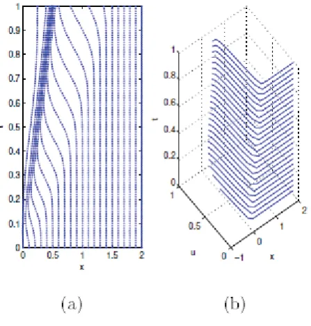
Fig. 1:The mesh trajectory and solution of the first example for 0≤t≤1.0 with adaptive level set method(MMPDE5) of 21 mesh point,(μ= 0.5, λ= 0.4, ε= 0.01, β= 0).
Example 4.1.Consider the Burger’s equation as first example,
ut+uux−εuxx= 0,
where its exact solution is:
u(x, t) = μ+λ+ (μ−λ)e
λ
ε(x−μt−β)
1 +eλε(x−μt−β) .
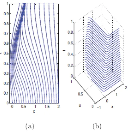
Fig. 2:The mesh trajectory and solution of the first example for 0≤t≤1.0 with adaptive level set method(MMPDE6) of 21 mesh point,(μ= 0.5, λ= 0.4, ε= 0.01, β= 0).
Table 1: The error of ALSM(with MMPDE5) for the first example att= 1.0, obtained by the arclength monitor function withα= 0(uniform mesh) andα= 2(moving mesh)without LTSR and with LTSR, (μ= 0.5, λ= 0.4, ε= 0.01 andβ= 0).
MMPDE Time stepping Type of mesh N L∞-error CPU time 21 0.1924 0.504 5 without LTSR fixed mesh 31 0.0782 0.612 (α= 0) 41 0.0564 0.8807
21 0.0711 0.7548 5 without LTSR Moving mesh 31 0.0602 0.8315 (α= 2) 41 0.0587 0.9812
21 0.0510 0.917 5 with LTSR Moving mesh 31 0.0347 1.019 (α= 2) 41 0.0298 1.079
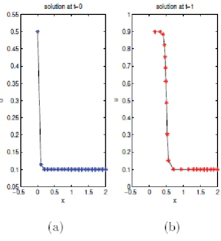
Fig. 3: The solution att= 0 with uniform mesh and att= 1 with adaptive level set method(MMPDE5) of 21 mesh point for the first example, (μ= 0.5, λ= 0.4, ε= 0.01, β= 0).
Table 2: The error of ALSM(with MMPDE6) for the first example at t = 1.0, ob-tained by the arclength monitor function withα= 0 (uniform mesh) andα= 2(moving mesh)without LTSR and with LTSR, (μ= 0.5, λ= 0.4, ε= 0.01 andβ= 0).
MMPDE Time stepping Type of mesh N L∞-error CPU time 21 0.0645 0.8815 6 without LTSR fixed mesh 31 0.0578 0.9205 (α= 0) 41 0.0512 0.9876
21 0.0441 0.031 6 without LTSR Moving mesh 31 0.0315 1.108 (α= 2) 41 0.0274 1.230
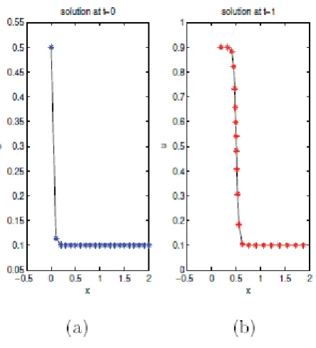
Fig. 4: The solution att= 0 with uniform mesh and att= 1 with adaptive level set method(MMPDE6) of 21 mesh point for the first example, (μ= 0.5, λ= 0.4, ε= 0.01, β= 0).
with LTSR gives better results. Similar information, are given in Table 2 when the MMPDE6 is applied for calculating nodes velocity. Figure 1(a) shows mesh trajectories for 0≤x≤2,0≤t≤1.0 which has been derived by using the new method with MMPDE5, also the solution of PDE,u, has been plotted on the moving mesh for 0≤t≤1.0 in Figure 1(b). The spatial do-main is divide into 21 mesh points. Like above, mesh trajectories and solution of Example 4.1 have been plotted by using the new method with MMPDE6 in Figure 2. Also in Figure 3 we plotted the solution of PDE at t = 0 on a uniform initial mesh and at t= 1 on a moving mesh with MMPDE5 and similarly, the solution att= 0 andt= 1 has been plotted with MMPDE6 in Figure 4.
For demonstrating the efficiency of our method we compare this method with another moving mesh method. For this purpose, we consider moving element free Petrov-Galerkin viscous method, MEFP-GVP, where introduced in [2], for comparing under equal conditions we consider the parametersμ, λ, εand
β in the Burger’s equation according to [2], (μ= 0.5, λ = 0.4, ε= 1/15 and
Fig. 5: The mesh trajectory and solution of the first example for 0 ≤ t ≤ 1.0 with adaptive level set method(MMPDE5) of 21 mesh point,(μ= 0.5, λ= 0.4, ε= 1/15, β= 0).
MEFP-GVM but in ALSM we have L∞- error= 0.01. This result shows the preference of our method. In addition, the CPU time in our method is very smaller than the MEFP-GVM. Also we plotted grid motion and the solution for new conditions for 21 grid points in Figure 5.
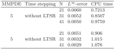
Table 3:The error of ALSM(with MMPDE5) for the second example att= 1.0, obtained by the arclength monitor function (α= 2) without LTSR and with LTSR.
MMPDE Time stepping N L∞-error CPU time 21 0.0060 0.7213 5 without LTSR 31 0.0052 0.8507 41 0.0050 0.9759
21 0.0051 0.906 5 without LTSR 31 0.0032 1.015 41 0.0029 1.076
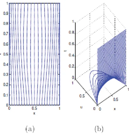
Fig. 6: The mesh trajectory and solution of the second problem for 0 ≤ x ≤ 1 and 0≤t≤1.0 with adaptive level set method(MMPDE5) of 21 mesh point.
Table 4:The error of ALSM(with MMPDE6) for the second example att= 1.0, obtained by the arclength monitor function (α= 2) without LTSR and with LTSR.
MMPDE Time stepping N L∞-error CPU time 21 0.0023 0.8706 6 without LTSR 31 0.0015 0.9844 41 0.0009 1.029
21 0.0048 1.025 6 without LTSR 31 0.0030 1.098 41 0.0024 1.221
ut=uxx,
with the exact solution:
u(x, t) =e−π2tsinπx
This problem has been used in [3] as a numerical example and also in [15] to study the moving mesh with variable relaxation time.
Fig. 7: The mesh trajectory and solution of the second problem for 0 ≤ x ≤ 1 and 0≤t≤1.0 with adaptive level set method(MMPDE6) of 21 mesh point.
M =1 +αu2x
we have M(x, t) → 1 as t → +∞ and so the equidistributed mesh should tend to a uniform mesh in space.
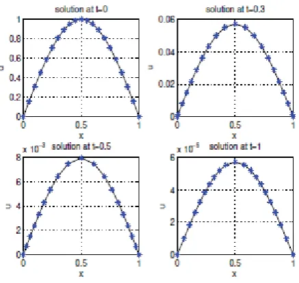
Similar to Tables 1 and 2, some results about the second example are given in Tables 3 and 4 which certify the quality of the new mesh adaptive algorithm. Figure 6(a) shows the mesh trajectories for the above problem using adaptive level set method with MMPDE5 and in Figure 6(b), the numerical solution of PDE is plotted for 0 ≤t≤1.0 by the new method with MMPDE6 have been plotted. We also plotted the solution at t= 0 on uniform initial mesh and at the timest = 0.3,0.5 andt = 1 on moving mesh in Figure 8. As we expect, the adaptive mesh at t= 1 tends towards uniform mesh.
In the second example, because of the smoothness of the solution there is not any major difference between the uniform and the adaptive mesh and also between the adaptive mesh with MMPDE5 and MMPDE6. In this example, ALSM with LTSR does not yield any different result from ALSM without LTSR.
Example 4.3.We use the following Burger’s equation as the third example,
Fig. 8:The solution of the second PDE att= 0,0.3,0.5 andt= 1 with its corresponding mesh nodes.
The initial condition is considered as follows [7]:
u(x,0) =|sin(2πx
xR )|.
The boundary conditions are chosen in the form
u(0, t) =u(xR, t) = 0.
We select ε = 10−5 and xR = 2 in this example. This example has been solved by the presented method up tot= 1.
The mesh trajectory has been plotted along with the nodes of moving grid with N = 21 mesh points in different times in Figure 9. Also the computed solution of the third example has been plotted in Figure 9. It is clear that the mesh moves correctly, because the solution has large variations aboutx= 0.5 andx= 2 and the mesh also concentrates around these areas.
5 Conclusion
In this paper, we have developed a static moving mesh method based on the level set approach for solving one dimensional time dependent PDEs, such that for representing the nodes of adaptive mesh, the level set equation is used. Also, we proposed a strategy for local time step refinement where the local time step is selected by the level set function. This adaptive method is among the static moving mesh. We plan to investigate the dynamical moving mesh method based on the level set function.
References
1. Aslam, T.,A level set algorithm for tracking discontinuities in hyperbolic conservation laws,I:Scalar equations, J. Comput. Phys.167, (2001), 413-438.
2. Ghorbani, M. and Soheili, A.R.,Moving element free Petrov Galerkian viscous method,special issue on meshless methodes, Journal of the Chinese Institue of en-gineers,27, (2004), 473-479.
3. Huang, W., Ren, Y. and Russell, R., Moving mesh partial differential equa-tions(MMPDEs)based on the equiditribution principle, SIAM J.Number. Anal.31, (1994), 709-730.
4. Huang, W., Ren, Y. and Russell, R.,Moving mesh methods based on moving mesh partial differential equations, J. Compute. Phys.,113, (1994), 279-290.
5. Jin, S. and Osher, S.,A level set method for the computation of multivalued solutions to quasi-linear hyperbolic PDEs and Hamilton-Jacobi equations, SIAM .Numer. Analys.
28, (1991), 907-921.
7. Mazhukin, A.V., Dynamic adaptation in convection-diffusion equations, Comput. method. Appl. Math,8, (2008), 171-186.
8. Mazhukin, A.V. and Chuiko, M.M.,Solution of the multi-interface Stefan problem by the method of dynamic adaptation, Compute. method. Appl. Math,2, (2002), 283-294. 9. Osher, S. and Fedkiw, R.,Level set methods and dynamic implicit surfaces,
Springer-Verlag, NY, (2002)
10. Osher, S. and Sanders, R.,Numerical approxiamtion to nonlinear conservation laws with locally varying time and spaces grid , Math. Compute.41, (1983), 321-336. 11. Osher, S. and Sethian, J., Front propagating with curvature dependent speed:
Algo-rithms based on Hamilton-Jacobi formulations, J. Compute. Phys.79, 12 (1988). 12. Sethian, J.A.Level set methods and fast marching methods, New York: Cambridge
University Press,(1999).
13. Soheili, A.R. and Ameri, M.A., Adaptive grid based on geometric conservation law level set method for time dependent PDE, Numerical methods for PDEs,25, (2009), 582-597.
14. Soheili, A.R. and Salahshour, S.,Moving mesh methods with local time step refinement for blow-up problems, Appl.Math.Copmpute.195, (2008), 76-85.
15. Soheili, A.R. and Stockie, J.M.,A moving mesh method with variable mesh relaxation time, Appl.Number.Math.58, (2008), 249-263.
16. Stockie, J.M., Mackenzie, J.A. and Russell, R.,A moving mesh method for one di-mensional hyperbolic conservation laws, SIAM. J.S.Compute.22, (2001), 1791-1831. 17. Tan, H.Z. and Tang, T.,Adaptive mesh methods for one- and two-dimensional
hyper-bolic conservation laws, SIAM. J.Numer. Anal.41, (2003), 487-515.
18. Tan, Z., Zhang, Z., Huang, Y. and Tang, T.,Moving mesh methods with locally varying time step, J. Comp. Phys.200, (2004), 347-367.