Galley
Pro
of
Vol. 9, No. 1, (2019), pp 127–150 DOI:10.22067/ijnao.v9i1.63182
Regularization technique and
numerical analysis of the mixed system
of first and second-kind
Volterra–Fredholm integral equations
S. Pishbin∗ and J. Shokri
Abstract
It is important to note that mixed systems of first and second-kind Volterra–Fredholm integral equations are ill-posed problems, so that solving discretized system of such problems has a lot of difficulties. We will apply the regularization method to convert this mixed system (ill-posed problem) to system of the second kind Volterra–Fredholm integral equations (well-posed problem). A numerical method based on Chebyshev wavelets is suggested for solving the obtained well-posed problem, and convergence analysis of the method is discussed. For showing efficiency of the method, some test prob-lems, for which the exact solution is known, are considered.
Keywords: Mixed systems of first and second-kind Volterra–Fredholm in-tegral equations; Regularization method; Chebyshev wavelets; Convergence analysis.
1 Introduction
The Volterra–Fredholm integral equations [4,5,7,13] arise from parabolic boundary value problems, from the mathematical modeling of the spatiotem-poral development of an epidemic, mathematical population dynamics, and from various physical and biological models.
∗Corresponding author
Received 8 March 2017; revised 29 August 2018; accepted 15 October 2018 S. Pishbin
Department of Mathematics, Faculty of Sciences, Urmia University, Urmia, P. O. Box 165, Iran. e-mail: [email protected]
J. Shokri
Department of Mathematics, Faculty of Sciences, Urmia University, Urmia, P. O. Box 165, Iran. [email protected]
Galley
Pro
of
In this paper, we consider mixed system of Volterra–Fredholm integral equations (VFIEs) consisting of first and second-kind VFIEs as follows:F(t, x) =AU(t, x) +
∫ t
0
∫
Ω
K(t, η, x, s)U(η, s)dsdη, t∈I= [0, T], x∈Ω,
(1) whereF(t, x) = [f(t, x), g(t, x)]T, U(t, x) = [u
1(t, x), u2(t, x)]T and
A=
[
1 0 0 0
]
, K(t, η, x, s) =
[
k11(t, η, x, s)k12(t, η, x, s)
k21(t, η, x, s)k22(t, η, x, s)
] .
Here, Ω denotes a (closed) bounded region in Rd (d= 1,2,3) with the
(piecewise) smooth boundary∂Ω.
The reformulation of the initial-boundary-value problem for the linear heat equation in a two-dimensional spatial domain Ω with the boundary∂Ω by single-layer techniques leads to a mixed system of Volterra–Fredholm in-tegral equations. Mixed systems of VFIEs are considered as the ill-posed problems. However, we will first apply the method of regularization that received a considerable amount of interest, especially in solving first kind integral equations. The method transforms mixed system to the system of second kind integral equations. The method of regularization was established independently by Phillips [12] and Tikhonov [14]. The method of regular-ization consists of replacing ill-posed problem by well-posed problem. Some numerical methods have been proposed for solving Volterra–Fredholm inte-gral equations of the second kind; see, for example, [2,6,8,10,11,15,16]. In this paper, the wavelet collocation method is developed for a mixed system of first and second kind Volterra–Fredholm integral equations.
The paper is organized as follows. In Section 2, we consider some applica-tions of Volterra–Fredholm integral equation and in Section 3, we introduce regularization technique to transform mixed system (1) into the system of second kind integral equations. In Section 4, a numerical method based on Chebyshev wavelets is applied for solving the obtained well-posed problem. The convergence analysis is given in Section 5 and the numerical experiments are carried out in Section 6, which will be used to verify the theoretical re-sults.
2 Some applications
We can consider Volterra–Fredholm integral equation of the first kind as a spacial case of system (1)(let u1 = 0, k12 = 0). The reformulation of
follow-Galley
Pro
of
ing form [3]:gΓ(t, θ) =
∫ t
0
∫ 1 0
K(t−s, X(θ)−X(s))U(s, ϕ)dϕds,
whereX(θ) is a smooth 1-periodic parametric representation of the boundary curve Γ =∂Ω, andgΓrepresents the function describing the given boundary
condition onI×∂Ω.
For the another example, you can consider the following integral equation [1]
f(x, t) = (Λ(t)−f∗(x)) =
∫ t
0
∫
Ω
F(t, τ)k(x, y)Φ(y, t)dydτ,
(x= ¯x(x1, x2, x3), y= ¯y(y1, y2, y3),(x, y)∈Ω, t∈[0, T],)
under the condition ∫
Ω
Φ(x, t)dx=P(t),
can be investigated from the contact problem of a rigid surface (G, ν) hav-ing an elastic material occupyhav-ing the domain Ω where f∗(x) describing the surface of stamp. This stamp impressed into an elastic layer surface (plane) by a variable known force with respect to time P(t) whose eccentricity of applicatione(t),(t∈[0, T]) that case rigid displacement Λ(t). Here Gis the displacement magnitude andν is Poisson’s coefficient.
3 Regularization technique
The linear operator defined by second equation in system (1) has not gener-ally a continuous inverse, so that it is difficult to obtain a precise numerical solution by classical discretization methods. Thus regularization techniques could be used instead to transform integral equations such as second equa-tion in system (1) into second-kind integral equaequa-tions. More precisely, we consider the following integral equations:
f(t, x) =u1(t, x) +
∫ t
0
∫
Ω
k11(t, η, x, s)u1(η, s)dsdη
+
∫ t
0
∫
Ω
k12(t, η, x, s)u2,ε(η, s)dsdη,
g(t, x) =εu2,ε(t, x) +
∫ t
0
∫
Ω
k21(t, η, x, s)u1(η, s)dsdη
+
∫ t
0
∫
Ω
k22(t, η, x, s)u2,ε(η, s)dsdη,
(2)
Galley
Pro
of
Under a hypothesis that will be clarified later, it can be proved that the solution u2,ε(x, t) of equation (2) converges (when ε → 0) to the solutionu2(x, t) of equation (1). Now, we consider the matrix form of equation (2) as
the following system of integral equations:
F(t, x) =EUε(t, x) +
∫ t
0
∫
Ω
K(t, η, x, s)Uε(η, s)dsdη, (3)
whereE=
[
1 0 0 ε ]
andUε(x, t) = [u1(x, t), u2,ε(x, t)]T.
We need the following definition and lemma to regularization technique. Definition 1. A self-adjoint operator κ:H →H, where H is a real Hilbert space, is called coercive if there exists a constantc >0such that
⟨κx, x⟩ ≥c∥x∥2, for allx∈H.
Lemma 1. Suppose that the integral operator of system (3) is continuous and coercive in a Hilbert space, whereF, U, Uε are defined. Then
• ∥Uε∥is bounded independently of ε;
• ∥Uε−U∥tends to 0 when ε→0.
Proof. From (3) we conclude the following:
∥E∥∥Uε∥=∥F−
∫ t
0
∫
Ω
KUεdsdη∥⩾−∥F∥+∥
∫ t
0
∫
Ω
KUεdsdη∥, (4)
The coercivity property of the integral operator implies
∥ ∫ t
0
∫
Ω
KUεdsdη∥⩾α∥Uε∥, (5)
whereαis the coercivity constant. From (4) and (5) we deduce
∥E∥∥Uε∥⩾α∥Uε∥ − ∥F∥; (6)
therefore it is obtained:
(α− ∥E∥)∥Uε∥⩽∥F∥,
which proves the first part of the lemma.
Now, for proving the second result, by using (1) and (3), we have
E(Uε−U) =−
∫ t
0
∫
Ω
Galley
Pro
of
where ˜U1(x, t) = [u1(x, t),0]T. By rearranging (7), we can write∫ t
0
∫
Ω
K(t, η, x, s)[Uε(η, s)−U(η, s)]dsdη=−E(Uε−U)−εU˜2, (8)
where, by using vectors operationsEU−U˜1 =εU˜2 is obtained, which ˜U2=
[0, u2]T. Taking the norm from the both side of (8) and using the coercivity
property imply
α∥Uε−U∥⩽∥E(Uε−U)−εU˜2∥⩽∥E∥∥Uε−U∥+ε∥U˜2∥. (9)
From∥U˜2∥=∥u2∥, we deduce that
(α− ∥E∥)∥Uε−U∥⩽ε∥u2∥, (10)
and now from∥E∥= 1 +ε→1 whenε→0 andα≫1 then it is concluded that ∥Uε−U∥ →0 when ε→0. This completes the proof.
The conditions of existence and uniqueness of solutions related to the VFIEs (3) can be investigated by considering the theorem about existence and uniqueness of solution of the second-kind Volterra–Fredholm integral equation in [3].
Theorem 1. Assume that 1. F ∈C(I×Ω)
2. K∈C(D×Ω2)whereD={(t, η),0≤η≤t≤T}.
Then the mixed system (3) possesses a unique solution Uε∈C(I×Ω).
4 Numerical treatment
4.1 Chebyshev wavelets
Dilations and translations of the “Mother function,” or “analyzing wavelet” Φ(x) define an orthogonal basis, our wavelet basis:
Φ(s,l)(t) = 2
−s
2 Φ(2−st−l),
the variablessandlare integers that scale and dilate the mother function Φ to generate wavelets, such as a Daubechies wavelet family. The scale indexs
Galley
Pro
of
ϕ(n,m) =ϕ(k, n, m, t) have four arguments, n= 1,2, . . . ,2k−1, where k can
assume any positive integer andm is the degree of Chebyshev polynomials of the first kind. They are defined on the interval [0,1) as
ϕ(n,m)(t) =
{
2k2Tˆm(2kt−2n+ 1), n−1
2k−1 ≤t <
n
2k−1,
0, otherwise, (11)
where
ˆ
Tm(t) =
{√1
π, m= 0,
√
2
πTm(t), m >0,
and m = 0,1, . . . , M −1, n = 1,2, . . . ,2k−1. Also T
m(t) are Chebyshev
polynomials of degree m which are orthogonal with respect to the func-tionw(t) = √1
1−t2 on the interval [−1,1]. We consider the two-dimensional Chebyshev waveletϕ(n1,m1,n2,m2)(x, y) as follows:
2k1 +2k2Tˆm 1(2
k1x−2n
1+ 1) ˆTm2(2
k2y−2n
2+ 1), 2nk11−−11 ≤x <
n1
2k1−1,
n2−1
2k2−1 ≤y <
n2
2k2−1,
0, otherwise,
(12) where m1 = 0,1, . . . , M1−1,m2 = 0,1, . . . , M2−1,n1 = 1, . . . ,2k1−1, and
n2= 1, . . . ,2k2−1.
A functionu(x, y)∈L2([0,1)×[0,1)) may be expanded as
u(x, y) =
∞ ∑
n1=1 ∞ ∑
m1=0 ∞ ∑
n2=1 ∞ ∑
m2=0
un1m1n2m2ϕ(n1,m1,n2,m2)(x, y). (13) If the infinite series in equation (13) is truncated, then
u(x, y)≈
2k1−1 ∑
n1=1
M∑1−1
m1=0
2k2−1 ∑
n2=1
M∑2−1
m2=0
un1m1n2m2ϕ(n1,m1,n2,m2)(x, y) = Φ(x)
TUΦ(y).
(14) where Φ(x) and Φ(y) are (2k1−1)M
1×1 and (2k2−1)M2×1 matrices,
respec-tively, such that
Φ(x) = [ϕ(1,0)(x), . . . , ϕ(1,M1−1)(x), . . . , ϕ(2k1−1,0)(x), . . . , ϕ(2k1−1,M
1−1)(x)]
T,
Φ(y) = [ϕ(1,0)(y), . . . , ϕ(1,M2−1)(y), . . . , ϕ(2k2−1,0)(y), . . . , ϕ(2k2−1,M 2−1)(y)]
T
.
AlsoU is a (2k1−1)M
1×(2k2−1)M2matrix whose elements can be calculated
as
un1m1n2m2 = ∫ 1
0
∫ 1 0
Galley
Pro
of
where n1 = 1, . . . ,2k1−1, m1 = 0,1, . . . , M1−1, n2 = 1, . . . ,2k2−1, m2 =0,1, . . . , M2−1 and
wn(t) =
{
w(2kt−2n+ 1), n−1 2k−1 ≤t <
n
2k−1,
0, otherwise
Now, consider system (2) with I= Ω = [0,1] and approximate the solu-tion of this system using (13) as
ˆ
u1(t, x) = Φ(t)TU1Φ(x). (15)
ˆ
u2,ε(t, x) = Φ(t)TU2,εΦ(x). (16)
Also, we approximate the kernels in system (2) respect to two variables η
andsas follows:
kij(t, η, x, s)≈kˆij(t, η, x, s) = Φ(η)TKijΦ(s) (i, j= 1,2). (17)
Inserting (15), (16), (17), and the following collocation points
ti=
i M12k1−1+ 1
, i= 1,2, . . . , M12k1−1,
xj=
j M12k2−1+ 1
, j= 1,2, . . . , M22k2−1, (18)
into system (2), we have the following linear system of algebraic equations for the unknown coefficientsU1andU2,ε:
f(ti, xj) = Φ(ti)TU1Φ(xj) +
∫ ti
0
∫ 1 0
ˆ
k11(ti, η, xj, s)Φ(η)TU1Φ(s)dsdη
+
∫ ti
0
∫ 1 0
ˆ
k12(ti, η, xj, s)Φ(η)TU2,εΦ(s)dsdη,
g(ti, xj) =εΦ(ti)TU2,εΦ(xj) +
∫ ti
0
∫ 1 0
ˆ
k21(ti, η, xj, s)Φ(η)TU1Φ(s)dsdη
+
∫ ti
0
∫ 1 0
ˆ
k22(ti, η, xj, s)Φ(η)TU2,εΦ(s)dsdη,
i= 1,2, . . . , M12k1−1, j= 1,2, . . . , M22k2−1.
(19)
4.2 Normalization
In the language of optimization theory, for the linear bounded operatorK:
Galley
Pro
of
Jε(x) =∥Kx−y∥2+ε∥x∥2, for allx∈X.
We can consider the following theorem from [9].
Theorem 2. Let K : X → Y be a linear bounded operator between Hilbert spaces and letϵ >0. Then the Thikhonov functional Jε has a unique
mini-mumxε∈X. This minimumxεis the unique solution of the normal equation
εxε+K∗Kxε=K∗y.
Here,K∗:Y →X denotes the adjoint ofK.
By using Theorem2, system (2) withI= Ω = [0,1] can be written in the normal form as follows:
f(p, q) =u1(p, q) +
∫ p
0
∫ 1 0
k11(p, η, q, s)u1(η, s)dsdη
+
∫ p
0
∫ 1 0
k12(p, η, q, s)u2,ε(η, s)dsdη,
∫ 1
p
∫ 1 0
k22(p, t, q, x)g(t, x)dxdt
=εu2,ε(p, q)
+ ∫ 1 p ∫ 1 0 ∫ t 0 ∫ 1 0
k22(p, t, q, x)k21(t, η, x, s)u1(η, s)dsdηdxdt
+ ∫ 1 p ∫ 1 0 ∫ t 0 ∫ 1 0
k22(p, t, q, x)k22(t, η, x, s)u2,ε(η, s)dsdηdxdt,
(20) Now, we can consider the numerical method based on Chebyshev wavelets from the previous subsection for the approximate solution of system (20).
5 Convergence analysis
In this section, we investigate the convergence analysis of the proposed Chebyshev wavelet collocation method, using polynomial approximation the-ory.
Lemma 2. Assume that u(x, y)∈L2([0,1)×[0,1)) can be expanded in the
form of series (13) and that uˆ(t, x)is the approximation of u(x, y) which is defined by (14). Thenuˆ(t, x)converges to u(t, x).
Proof. We recall the seriesu(t, x) from (13) and the truncated series ˆu(t, x) from (14), respectively, as follows:
u(x, y) =
∞ ∑
n1=1 ∞ ∑
m1=0 ∞ ∑
n2=1 ∞ ∑
m2=0
Galley
Pro
of
andˆ
u(t, x) =
2k1−1 ∑
n1=1
M∑1−1
m1=0
2k2−1 ∑
n2=1
M∑2−1
m2=0
un1m1n2m2ϕ(n1,m1,n2,m2)(t, x),
where m1 = 0,1, . . . , M1−1, m2 = 0,1, . . . , M2 −1, n1 = 1, . . . ,2k1−1,
andn2 = 1, . . . ,2k2−1. The functions ϕ(n1,m1,n2,m2)(t, x) are the Chebyshev wavelet. LetL2([0,1)×[0,1)) be the Hilbert space and let
ϕ(n1,m1,n2,m2)(t, x) = 2
−(n1 +n2 ) 2 ϕ(2
−n1
2 t−m1)ϕ(2 −n2
2 x−m2), whereϕ(n1,m1,n2,m2)(t, x) form a basis ofL
2([0,1)×[0,1)) as in (12).
From (13), we consider
u(t, x) =
∞ ∑
m1=0 ∞ ∑
m2=0
u1m11m2ϕ(1,m1,1,m2)(t, x) = ∞ ∑ i=0 ∞ ∑ j=0
cijϕ(i,j)(t, x),
where cij =< u(t, x), ϕ(i,j)(t, x) > for k1 = 1, k2 = 1 and < ., . >
rep-resents an inner product. Let us denote ϕ(i,j)(t, x) = ϕ(t, x) and αij =<
u(t, x), ϕ(t, x)>.
Define the sequence of partial sumsSn,m, n > m of {αijϕ(ti, xj)}. Let
Sn1,m1 and Sn2,m2 be arbitrary partial sums with n1 > n2. We show that Sn,m is a Cauchy sequence in a Hilbert space.
LetSn,m=
∑n1
i=0
∑n2
j=0αijϕ(ti, xj). From
< u(t, x),
n1 ∑ i=0 n2 ∑ j=0
αijϕ(ti, xj)>= n1 ∑ i=0 n2 ∑ j=0
|αij|2,
we can show that ∥Sn1,n2−Sm1,m2∥
2 =∑n1
i=m1+1 ∑n2
j=m2+1|αij|
2 for n 1 >
m1, n2> m2.
We can write
∥
n1 ∑
i=m1+1
n2 ∑
j=m2+1
αijϕ(ti, xj)∥2
=<
n1 ∑
i=m1+1
n2 ∑
j=m2+1
αijϕ(ti, xj), n1 ∑
i=m1+1
n2 ∑
j=m2+1
αijϕ(ti, xj)>
=
n1 ∑
i=m1+1
n2 ∑
j=m2+1
|αij|2,
Galley
Pro
of
∥
n1 ∑
i=m1+1
n2 ∑
j=m2+1
αijϕ(ti, xj)∥2= n1 ∑
i=m1+1
n2 ∑
j=m2+1
|αij|2,
forn1> m1, n2> m2.
Now from Bessel’s inequality, we deduce that ∑n1
i=m1+1 ∑n2
j=m2+1|αij|
2 is
convergent and therefore∥∑n1
i=m1+1 ∑n2
j=m2+1αijϕ(ti, xj)∥
2→0,
that is, ∥∑n1
i=m1+1 ∑n2
j=m2+1αijϕ(ti, xj)∥ → 0 and {Sn,m} is a Cauchy se-quence thus it converges to a real number like ‘s‘.
In the continuance, we prove that u(t, x) =s.
< s−u(t, x), ϕ(ti, xi)>=< s, ϕ(ti, xi)>−< u(t, x), ϕ(ti, xi)>
=< lim
n→∞Sn,m, ϕ(ti, xi)>−αij
= lim
n→∞< Sn,m, ϕ(ti, xi)>−αij =αij−αij = 0;
then it is concluded thatu(t, x) =sor ∑n1
i=0
∑n2
j=0αijϕ(ti, xj) converges to
u(t, x), and by induction it is evident that this result is established for any integer numbers ofk1andk2, so fork1→ ∞andk2→ ∞. In the other hand,
we can consider ˆu(t, x) asSn,m, which means ˆu(t, x) converges tou(t, x) and
this completes the proof.
Theorem 3. Consider a function u(x, y)∈L2([0,1]×[0,1]), with bounded
forth partial derivations, |∂∂42ux∂(x,y2y)| < B. Then the wavelet coefficient, un1m1n2m2 in (14) , decay as follows:
|un1m1n2m2| ≤
πB
24(n
1n2)5/2(m21−1)(m22−1)
. (21)
Proof. From (14) it follows that
un1m1n2m2 = ∫ 1
0
∫ 1 0
u(x, y)ϕ(n1,m1)(x)ϕ(n2,m2)(y)wn1(x)wn2(y)dydx =
∫ 1 0
ϕ(n1,m1)(x)wn1(x) ( ∫ 1
0
u(x, y)ϕ(n2,m2)(y)wn2(y)dy )
dx.
=
∫ 1 0
ϕ(n1,m1)(x)wn1(x)
( ∫ n2/2k2−1
(n2−1)/2k2−1
2k2/2u(x, y) ˆ
Tm2(2
k2y−2n
2+ 1)
wn2(2
k2y−2n
2+ 1)dy
) dx.
Galley
Pro
of
un1m1n2m2 = 1 2k2/2
∫ 1
0
ϕ(n1,m1)(x)wn1(x) [ ∫ π
0
u(x,cosθ2n2−1
2k2 ) √
2
πcosm2θ dθ
]
=
√
2 2k2/2√π
∫ 1
0
ϕ(n1,m1)(x)wn1(x) [
u(x,cosθ+ 2n2−1
2k2 )( sinm2θ
m2 ) π 0 + √ 2 23k2/2m2√π
∫ π
0
∂u(x,(cosθ2n2−1)/2k2)
∂y sinm2θsinθ dθ
]
dx
= 1
23k2/2m2√2π
∫ 1
0
ϕ(n1,m1)(x)wk1(x) [ ∫π
0
∂u(x,(cosθ2n2−1)/2k2)
∂y
(sin(m2−1)θ
m2−1 −
sin(m2+ 1)θ m2+ 1
)π
0
+ 1
25k2/2m2√2π
∫ π
0
∂2u(x,(cosθ+ 2n2−1)/2k2)
∂2y hm2(θ)dθ ]
dx,
(23) where
hm(θ) = sinθ
(sin(m
2−1)θ
m2−1 −
sin(m2+ 1)θ
m2+ 1
) .
Then, we obtain
un1m1n2m2 =
1 25k2/2m2√2π
∫ π
0
[ ∫1 0
∂2u(x,(cosθ+2n
2−1)/2k2)
∂2y
ϕ(n1,m1)(x)wk1(x)dx ]
hm2(θ)dθ. (24)
Now, similar to the discussion in (23), by substituting 2k1y−2n
1+ 1 = cosα
in (24), it yields
un1m1n2m2
= 1
25(k1+k2)/2m1m2(2π)
×∫ π 0
∫ π
0
∂4u((cosα+ 2n1−1)/2k1,(cosθ+ 2n2−1)/2k2)
∂2x∂2y hm1(α)hm2(θ)dα dθ.
Thus we have
|un1m1n2m2|
= 1
25(k1+k2)/2m1m2(2π) ∫ π 0 ∫ π 0
∂4u((cosα+ 2n1−1)/2k1,(cosθ+ 2n2−1)/2k2)
∂2x∂2y hm1(α)hm2(θ)dα dθ
≤ B
25(k1+k2)/2m1m2(2π) ∫ π
0
|hm1(α)|dα ∫ π
0
|hm2(θ)|dθ.
(25)
However
∫ π
0
|hm2(θ)|dθ= ∫ π
0
sinθ
(sin(m
2−1)θ
m2−1
−sin(m2+ 1)θ
m2+ 1
)dθ
≤ ∫ π
0
sinθsin(m2−1)θ
m2−1
+sinθsin(m2+ 1)θ
m2+ 1
≤ 2m2π
(m2 2−1)
,
Galley
Pro
of
and similarly, it is obtained∫ π
0
|hm1(α)|dα≤
2m1π
(m2 1−1)
. (27)
Sincen1≤2k1−1 andn2 ≤2k2−1, by substituting (26) and (27) in (25), the
desired result is obtained as follows:
|un1m1n2m2| ≤
2πB
25(k1+k2)/2(m2
1−1)(m 2 2−1)
.
Theorem 4. Letu(x, y)∈L2([0,1]×[0,1]), with bounded forth partial deriva-tions, |∂∂42ux∂(x,y2y)|< B; then the error bound would be obtained as follows:
σk1,M1,k2,M2 =O (
2−52(k1+k2) )
, (28)
where
σk1,M1,k2,M2 =
( ∫ 1 0
∫ 1 0
[
u(x, y)−
2k1−1 ∑
n1=1
M∑1−1
m1=0
2k2−1 ∑
n2=1
M∑2−1
M2=0
un1m1n2m2ϕ(n1,m1)(x)ϕ(n2,m2)(y) ]2
wn1(x)wn2(y)dx dy )1
2 .
Proof. From the error statement, we have
σ2
k1,M1,k2,M2
= ∫ 1 0 ∫ 1 0 [
u(x, y)−
2k1−1 ∑
n1=1
M∑1−1
m1=0 2k2−1
∑
n2=1
M∑2−1
M2=0
un1m1n2m2ϕ(n1,m1)(x)ϕ(n2,m2)(y) ]2
wn1(x)wn2(y)dx dy
= ∫ 1 0 ∫ 1 0 [ ∑∞
n1=1 ∞ ∑
m1=0 ∞ ∑
n2=1 ∞ ∑
M2=0
un1m1n2m2ϕ(n1,m1)(x)ϕ(n2,m2)(y)
− 2k1−1
∑
n1=1
M∑1−1
m1=0 2k2−1
∑
n2=1
M∑2−1
m2=0
un1m1n2m2ϕ(n1,m1)(x)ϕ(n2,m2)(y) ]2
wn1(x)wn2(y)dx dy
= ∫ 1 0 ∫ 1 0 ∞ ∑
n1=2k1 ∞ ∑
m1=M1 ∞ ∑
n2=2k2 ∞ ∑
m2=M2
u2n1m1n2m2(ϕ(n1,m1)(x))
2(ϕ(
n2,m2)(y))
2
wn1(x)wn2(y)dx dy
=
∞ ∑
n1=2k1 ∞ ∑
m1=M1 ∞ ∑
n2=2k2 ∞ ∑
m2=M2
u2n1m1n2m2 ∫ 1
0
∫ 1
0
(ϕ(n1,m1)(x))
2(ϕ
(n2,m2)(y))
Galley
Pro
of
wn1(x)wn2(y)dx dy
=
∞ ∑
n1=2k1 ∞ ∑
m1=M1 ∞ ∑
n2=2k2 ∞ ∑
m2=M2
u2n1m1n2m2 ∫ n1
2k1−1 n1−1 2k1−1
[
2k21Tˆm1(2
k1x−2n1+ 1) ]2
√
1−(2k1x−2n1+ 1)2
dx
×∫ n2 2k2−1 n2−1 2k2−1
[
2k22Tˆm2(2k2y−2n2+ 1) ]2
√
1−(2k2x−2n2+ 1)2 dy
=
∞ ∑
n1=2k1 ∞ ∑
m1=M1 ∞ ∑
n2=2k2 ∞ ∑
m2=M2
u2n1m1n2m22 k1+k2
∫ n1 2k1−1 n1−1 2k1−1
[ ˆ
Tm1(2
k1x−2n1+ 1) ]2
√
1−(2k1x−2n1+ 1)2
dx
×
∫ n2 2k2−1 n2−1 2k2−1
[ ˆ
Tm2(2k2y−2n2+ 1) ]2
√
1−(2k2x−2n2+ 1)2dy.
Now, let 2k1y−2n
1+ 1 =t1and 2k2y−2n2+ 1 =t2, then it is obtained
sigma2k1,M1,k2,M2 = ∞ ∑
n1=2k1 ∞ ∑
m1=M1 ∞ ∑
n2=2k2 ∞ ∑
m2=M2
u2n1m1n2m2 ∫ 1
−1
ˆ
Tm1(t1) √
1−t2 1
dt1
∫ 1
−1
ˆ
Tm2(t2) √
1−t2 2
dt2.
(29) Form1≥1, m2≥1, we have
∫ 1
−1
ˆ
Tm1(t1) √
1−t2 1
dt1=
π
2,
∫ 1
−1
ˆ
Tm2(t2) √
1−t2 2
dt2=
π
2;
then (29) simplifies as follows:
σk21,M1,k2,M2 = π2
4
∞ ∑
n1=2k1 ∞ ∑
m1=M1 ∞ ∑
n2=2k2 ∞ ∑
m2=M2
u2n1m1n2m2. (30) Therefore from (21) and (30), we can conclude the desired result as follows:
σk2
1,M1,k2,M2≤ π4B
210
∞ ∑
n1=2k1 ∞ ∑
m1=M1 ∞ ∑
n2=2k2 ∞ ∑
m2=M2
1
(n1n2)5(m12−1)2(m22−1)2
.
(31) Also
∞ ∑
n1=2k1 1 (n1)5
= 1
(2k1)5 + 1
(2k1+ 1)5. . .= 1 (2k1)5
∞ ∑
n=0
1 (1 +2nk1)
5. (32)
Galley
Pro
of
σk1,M1,k2,M2 =O (
2−52(k1+k2) )
.
Theorem 5. Let us consider M = max∥K(t, η, x, s)∥, for η, t ∈ I = [0,1], s, x ∈ Ω = [0,1]. Assume that Uε(t, x) is the exact solution of
sys-tem (3) and that Uˆε(t, x) denotes the Chebyshev wavelet approximation for
the exact solutionU which is given by (15) and (16) . ThenUˆε(t, x)converges
toUε(t, x)and the following result can be obtained
∥Uε−Uˆε∥=O
(
2−52(k1+k2) )
.
Proof. According to the proposed method in previous section, we consider (15), (16), and (17) and insert ˆUε(t, x) andK(ˆ t, η, x, s) as approximations of
the exact solutionU and kernelKinto system (3)
F(t, x) =EUε(t, x) +
∫ t
0
∫ 1 0
ˆ
K(t, η, x, s)Uε(η, s)dsdη. (33)
Subtracting (3) from (33) and some manipulations, we get
∥E∥∥Uε−Uˆε∥⩽∥
∫ t
0
∫ 1 0
(K(t, η, x, s)−K(ˆ t, η, x, s))Uε(η, s)dsdη∥
+∥
∫ t
0
∫ 1 0
ˆ
K(t, η, x, s)(Uε(η, s)−Uˆε(η, s))dsdη∥.
From∥E∥ ≥1 it is obtained
∥Uε−Uˆε∥⩽∥K−Kˆ∥∥Uε∥+M∥Uε−Uˆε∥. (34)
Relation (34) together with Lemma2, shows the convergence of the exact solution to the approximate solution. Considering Theorem4, we have
∥K−Kˆ∥=O (
2−52(k1+k2) )
. (35)
From (34) and (35), we conclude that
∥Uε−Uˆε∥=O
(
2−52(k1+k2) )
Galley
Pro
of
6 Numerical examples
To demonstrate the efficiency and the practicability of the proposed method, we consider the following two examples. All results are computed by using a program written in the Mathematica®.
Example 1. Consider the following TIAEs:
∫ t
0
∫ 1 0
100t(t+x)u(η, s)dsdη=25 3 t
2(3 + 4t)(t+x), t∈[0,1], (36)
where the exact solution isu(t, x) =t+x.
Considering regularization techniques and (3) for (36), we have
εuε(t, x) +
∫ t
0
∫ 1 0
100t(t+x)u(η, s)dsdη= 25 3 t
2(3 + 4t)(t+x). (37)
We assume that ˆuε(t, x) is the approximation of the exact solutionuε(t, x)
which is defined by (15). For analyzing the behavior of the error representa-tions, we consider absolute error as
Error=|u(ti, xj)−uˆε(ti, xj)|.
The Chebyshev wavelet method described in Section4 has been imple-mented for problem (37) with M1 =M2 = 3, k1 =k2= 2 and the error for
different values ofεhas been reported in Table1, which confirms the theoret-ical results of Lemma1. Figure1presents the plots of exact and approximate solution withε= 0.000001, which are found to be in good agreement.
From subsection 4.2, we consider the normal form of equation (36) as follows:
εuε(p, q) +
∫ 1
p
∫ 1 0
∫ t
0
∫ 1 0
10000pt(p+q)(t+x)uε(η, s)dsdηdxdt
=
∫ 1
p
∫ 1 0
2500
3 p(p+q)t
2(3 + 4t)(t+x)dxdt, p∈[0,1],
(38)
and then solve this equation by the Chebyshev wavelet method with M1 =
M2= 3 andk1=k2= 2. We report the error for different values ofεin Table
2. From numerical results in Tables1 and 2, we observe that the results in Table2 are more accurate than the reported results in Table1.
Example 2. Consider the following:
Au(t, x) +
∫ t
0
∫ 1 0
Galley
Pro
of
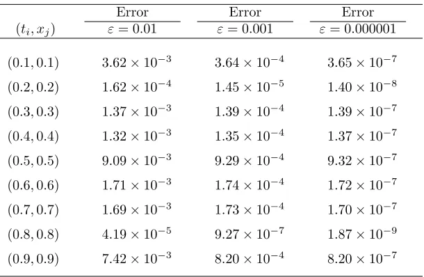
Table 1: Absolute errors ofuεfor different values ofεin Example 1Error Error Error
(ti, xj) ε= 0.01 ε= 0.001 ε= 0.000001
(0.1,0.1) 3.62×10⁻³ 3.64×10⁻⁴ 3.65×10⁻⁷
(0.2,0.2) 1.62×10⁻⁴ 1.45×10⁻⁵ 1.40×10⁻⁸ (0.3,0.3) 1.37×10⁻³ 1.39×10⁻⁴ 1.39×10⁻⁷
(0.4,0.4) 1.32×10⁻³ 1.35×10⁻⁴ 1.37×10⁻⁷ (0.5,0.5) 9.09×10⁻³ 9.29×10⁻⁴ 9.32×10⁻⁷
(0.6,0.6) 1.71×10⁻³ 1.74×10⁻⁴ 1.72×10⁻⁷
(0.7,0.7) 1.69×10⁻³ 1.73×10⁻⁴ 1.70×10⁻⁷
(0.8,0.8) 4.19×10⁻⁵ 9.27×10⁻⁷ 1.87×10⁻⁹
(0.9,0.9) 7.42×10⁻³ 8.20×10⁻⁴ 8.20×10⁻⁷
Table 2: Absolute errors ofuεfor different values ofεfor normal equation in Example 1
Error Error Error
(ti, xj) ε= 0.01 ε= 0.001 ε= 0.000001
(0.1,0.1) 6.18×10⁻⁶ 6.11×10⁻⁶ 1.95×10⁻⁷
(0.2,0.2) 6.84×10⁻⁶ 6.26×10⁻⁶ 5.22×10⁻⁸ (0.3,0.3) 3.79×10⁻⁶ 3.83×10⁻⁷ 8.93×10⁻⁸
(0.4,0.4) 2.43×10⁻⁵ 2.43×10⁻⁶ 5.70×10⁻⁸ (0.5,0.5) 2.06×10⁻⁵ 2.06×10⁻⁶ 6.66×10⁻⁷
(0.6,0.6) 2.14×10⁻⁵ 2.14×10⁻⁶ 2.42×10⁻⁷
(0.7,0.7) 7.78×10⁻⁶ 7.78×10⁻⁷ 1.67×10⁻⁷
(0.8,0.8) 2.25×10⁻⁵ 2.25×10⁻⁶ 2.41×10⁻⁸
Galley
Pro
of
whereA=
[
1 0 0 0
]
, K(t, η, x, s) =
[
η2(s2+t2+ 1) (s+t)
ηs2+η+ηt2 200s+ 200t
] ,
u(t, x) =(u1(t, x), u2(t, x)
)T
, f(t, x) =(f1(t, x), f2(t, x)
)T
,
andf1andf2are such that the exact solution is
u1(t, x) =t2+x2+ 1, u2(t, x) =t+x.
We apply the regularization method to convert the mixed system (39) to the system of the second kind integral equations. Then, the resulting second kind integral equation will be solved by the proposed numerical scheme in section 4 with M1 = M2 = 3 and k1 = k2 = 2 . Let (ˆu1,uˆ2,ε) be the
approximation of the exact solution (u1, u2,ε) which are defined by (15) and
(16). Numerical errors with several values ofεare displayed in Tables3 and 4.
Figure 1: The plots of exact solutionuand approximate solution ofuwithε= 0.000001 in Example 1.
Galley
Pro
of
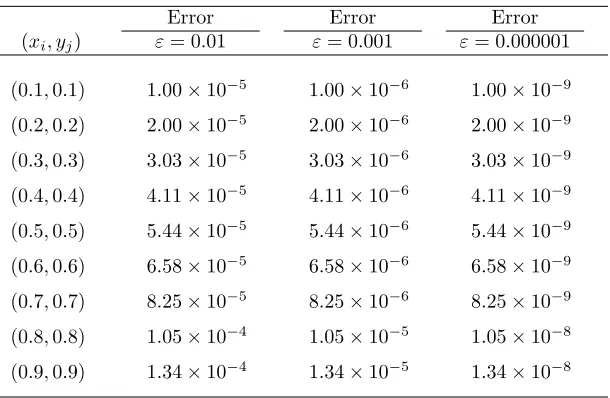
Table 3: Absolute errors ofu1 for different values ofεin Example 2Error Error Error
(xi, yj) ε= 0.01 ε= 0.001 ε= 0.000001
(0.1,0.1) 1.00×10⁻⁵ 1.00×10⁻⁶ 1.00×10⁻⁹
(0.2,0.2) 2.00×10⁻⁵ 2.00×10⁻⁶ 2.00×10⁻⁹ (0.3,0.3) 3.03×10⁻⁵ 3.03×10⁻⁶ 3.03×10⁻⁹
(0.4,0.4) 4.11×10⁻⁵ 4.11×10⁻⁶ 4.11×10⁻⁹ (0.5,0.5) 5.44×10⁻⁵ 5.44×10⁻⁶ 5.44×10⁻⁹
(0.6,0.6) 6.58×10⁻⁵ 6.58×10⁻⁶ 6.58×10⁻⁹
(0.7,0.7) 8.25×10⁻⁵ 8.25×10⁻⁶ 8.25×10⁻⁹
(0.8,0.8) 1.05×10⁻⁴ 1.05×10⁻⁵ 1.05×10⁻⁸
(0.9,0.9) 1.34×10⁻⁴ 1.34×10⁻⁵ 1.34×10⁻⁸
Table 4: Absolute errors ofu2,εfor different values ofεin Example 2
Error Error Error
(xi, yj) ε= 0.01 ε= 0.001 ε= 0.000001
(0.1,0.1) 1.07×10⁻³ 1.83×10⁻⁴ 8.51×10⁻⁶
(0.2,0.2) 1.58×10⁻⁴ 2.84×10⁻⁵ 1.86×10⁻⁵ (0.3,0.3) 2.39×10⁻⁴ 2.36×10⁻⁵ 1.78×10⁻⁵
(0.4,0.4) 4.63×10⁻⁴ 2.48×10⁻⁵ 2.37×10⁻⁶ (0.5,0.5) 3.84×10⁻³ 8.20×10⁻⁴ 4.82×10⁻⁵
(0.6,0.6) 1.66×10⁻³ 1.12×10⁻⁴ 1.06×10⁻⁴
(0.7,0.7) 1.22×10⁻³ 1.80×10⁻⁴ 1.77×10⁻⁴
(0.8,0.8) 2.85×10⁻³ 2.81×10⁻⁴ 1.80×10⁻⁴
Galley
Pro
of
Figure 2: The plots of exact solutionu1and approximate solution ofu1withε= 0.000001 in Example 2.
Table 5: Absolute errors ofu1for different values ofεfor normal equation in Example 2
Error Error Error
(xi, yj) ε= 0.01 ε= 0.001 ε= 0.000001
(0.1,0.1) 8.54×10⁻⁸ 8.54×10⁻⁹ 8.54×10⁻¹²
(0.2,0.2) 2.56×10⁻⁸ 2.56×10⁻⁹ 2.56×10⁻¹² (0.3,0.3) 4.19×10⁻⁸ 4.19×10⁻⁹ 4.19×10⁻¹²
(0.4,0.4) 1.10×10⁻⁷ 1.10×10⁻⁸ 1.10×10⁻¹¹ (0.5,0.5) 5.46×10⁻⁷ 5.46×10⁻⁸ 5.46×10⁻¹¹
(0.6,0.6) 1.73×10⁻⁶ 1.73×10⁻⁷ 1.73×10⁻¹⁰
(0.7,0.7) 2.54×10⁻⁶ 2.54×10⁻⁷ 2.54×10⁻¹⁰
(0.8,0.8) 2.86×10⁻⁶ 2.86×10⁻⁷ 2.86×10⁻¹⁰
(0.9,0.9) 2.58×10⁻⁶ 2.58×10⁻⁷ 2.58×10⁻¹⁰
Galley
Pro
of
Figure 3: The plots of exact solutionu2and approximate solution ofu2withε= 0.000001 in Example 2.
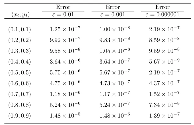
and 5, 6, we observe that the results in Tables 5 and 6 are more accurate than the reported results in Tables3 and4. This is predicted by the theory, in particular by Theorem2. Figures2 and 3 present the plots of exact and approximate solution withε= 0.000001.
6.1 Haar wavelet method
Galley
Pro
of
Table 6: Absolute errors ofu2,εfor different values ofεfor normal equation in Example 2Error Error Error
(xi, yj) ε= 0.01 ε= 0.001 ε= 0.000001
(0.1,0.1) 1.25×10⁻⁷ 1.00×10⁻⁸ 2.19×10⁻⁷
(0.2,0.2) 9.92×10⁻⁷ 9.83×10⁻⁸ 8.59×10⁻⁸
(0.3,0.3) 9.58×10⁻⁸ 1.05×10⁻⁸ 9.59×10⁻⁸ (0.4,0.4) 3.64×10⁻⁶ 3.64×10⁻⁷ 5.67×10⁻⁹
(0.5,0.5) 5.75×10⁻⁶ 5.67×10⁻⁷ 2.19×10⁻⁷ (0.6,0.6) 4.75×10⁻⁶ 4.73×10⁻⁷ 4.37×10⁻⁷
(0.7,0.7) 1.18×10⁻⁶ 1.17×10⁻⁷ 1.52×10⁻⁷ (0.8,0.8) 5.24×10⁻⁶ 5.24×10⁻⁷ 7.34×10⁻⁸
(0.9,0.9) 1.48×10⁻⁵ 1.48×10⁻⁶ 1.39×10⁻⁷
hi(t) =
1, t∈[τ1, τ2],
−1, t∈[τ2, τ3],
0, elsewhere
where
τ1=
k
m, τ2= k+12
m , τ3= k+ 1
m .
The integerm= 2j, j= 0,1, . . . , pandk= 0,1, . . . , m−1 are the level of the wavelet and translation parameter, respectively. The indexiis calculated from the formulai=m+k+ 1 and the maximal value isi= 2M(M = 2p).
The index i = 1 corresponds to the scaling function of the Haar wavelet
h1(t) = 1. We can consider an approximate solution of equation (37) as
ˆ
uϵ(t, x) =
2∑M1
i=1 2∑M2
j=1
aijhi(t)hj(x),
where the coefficientsaij can be obtained by inserting approximate solution
ˆ
uϵ(t, x) and the following collocation points in equation (37)
tl=
l−(12) 2M1
, l= 1,2, . . . ,2M1, xr=
r−(12) 2M2
Galley
Pro
of
By assuming M1 =M2 = 4, the absolute error for different values of εhave been reported in Table 7. From Tables 1 and 7, we observe that the results obtained by the Chebyshev wavelet method are more accurate than the Haar wavelet method in this case.
Table 7: Absolute errors ofuεfor different values ofεby Haar wavelet method in Example 1
Error Error Error
(ti, xj) ε= 0.01 ε= 0.001 ε= 0.000001
(0.1,0.1) 8.99×10⁻² 8.07×10⁻² 7.99×10⁻²
(0.2,0.2) 8.83×10⁻² 2.11×10⁻² 1.41×10⁻² (0.3,0.3) 4.04×10⁻² 1.72×10⁻² 1.29×10⁻²
(0.4,0.4) 9.33×10⁻² 7.99×10⁻² 7.82×10⁻² (0.5,0.5) 4.99×10⁻¹ 5.00×10⁻¹ 4.99×10⁻¹
(0.6,0.6) 9.58×10⁻² 8.25×10⁻² 8.08×10⁻²
(0.7,0.7) 6.79×10⁻² 1.98×10⁻² 1.15×10⁻²
(0.8,0.8) 5.09×10⁻² 1.78×10⁻² 1.77×10⁻²
(0.9,0.9) 9.26×10⁻² 8.01×10⁻² 7.84×10⁻²
7 Conclusion and future work
This work has been concerned with the regularization method to convert the mixed systems of the first and second-kind Volterra–Fredholm integral equa-tions to the system of the second-kind Volterra–Fredholm integral equaequa-tions. We presented the numerical method based on Chebyshev wavelets for solving the obtained second-kind problem. Convergence of the method was proved. These results were confirmed by some numerical examples.
In the present work, we considered the mixed system (1) in special case with A =
[
1 0 0 0
]
Galley
Pro
of
Acknowledgements
The authors would like to express their gratitude for the referees of the paper for their valuable suggestions that improved the final form of the paper.
References
1. M.A. Abdou, F.A. Salama,Volterra–Fredholm integral equation of the first kind and spectral relationships, Appl. Math. Comput. 153 (2004), 141–153.
2. J. Ahmadi Shali, P. Darania, A.A. Jodayree, Collocation method for nonlinear Volterra–Fredholm integral equations, Open J. Appl. Sci. 2 (2012),115–121.
3. H. Brunner, Collocation methods for Volterra integral and related func-tional equations, Cambridge Monographs on Applied and Computafunc-tional Mathematics, vol. 15, Cambridge University Press, Cambridge, 2004. 4. O. Diekman, Thresholds and traveling waves for the geographical spread of
infection, J. Math. Biol. 6 (1978), 109–130.
5. M. Hamina, J. Saranen ,On the spline collocation method for the single-layer heat operator equation, Math. Comp. 62 (1994), 41–64.
6. L. Hocia, On Approximate Solution for Integral Equation of the Mixed Type, ZAMM J. Appl. Math. Mech. 76 (1996), 415–416.
7. Y, Iso, K. Onishi, On the stability of the boundary element collocation method applied to the linear heat equation, J. Comput. Appl. Math. 38 (1991), 201–209
8. J.P. Kauthen,Continuous time collocation for Volterra–Fredholm integral equations, Numer. Math. 56 (1989), 409–424.
9. A. Kirsch,An introduction to the mathematical theory of inverse problem, Second edition. Applied Mathematical Sciences, 120. Springer, New York, 2011.
10. K. Maleknejad, H. Almasieh, M. Roodaki, Triangular functions (TF) method for the solution of nonlinear Volterra–Fredholm integral equations, Commun. Nonlinear Sci. Numer. Simul. 15 (2010), 3293–3298
Galley
Pro
of
12. D.L. Phillips, A technique for the numerical solution of certain integralequations of the first kind, J. Assoc. Comput. Mach. 9 (1962), 84–97.
13. H. R. Thieme, A model for the spatio spread of an epidemic, J. Math. Biol. 4, (1977), 337–351.
14. A. N. Tikhonov, On the solution of incorrectly posed problem and the method of regularization, Soviet Math. 4 (1963), 1035–1038.
15. S. Yousefi, M. Razzaghi, Legendre Wavelets method for the nonlinear Volterra–Fredholm integral equations, Math. Comput. Simul. 70 (2005), 1–8.
مود و لوا عﻮﻧ ﻢﻠﻫدﺮﻓ-اﺮﺘﻟو ﯽﻟاﺮﮕﺘﻧا تﻻدﺎﻌﻣ ﺐﮐﺮﻣ هﺎﮕﺘﺳد یدﺪﻋ ﻞﯿﻠﺤﺗ و یزﺎﺳ ﻢﻈﻨﻣ
یﺮﮑﺷ داﻮﺟ و ﻦﯿﺑ ﺶﯿﭘ ﺪﯿﻌﺳ
ﯽﺿﺎﯾر هوﺮﮔ ،مﻮﻠﻋ هﺪﮑﺸﻧاد ،ﻪﯿﻣورا هﺎﮕﺸﻧاد
١٣٩٧ ﺮﻬﻣ ٢٣ ﻪﻟﺎﻘﻣ شﺮﯾﺬﭘ ،١٣٩٧ ﺮﻬﻣ ٧ هﺪﺷ حﻼﺻا ﻪﻟﺎﻘﻣ ﺖﻓﺎﯾرد ،١٣٩۵ ﺪﻨﻔﺳا ١٨ ﻪﻟﺎﻘﻣ ﺖﻓﺎﯾرد
ﺰﺟ مود و لوا عﻮﻧ ﻢﻠﻫدﺮﻓ-اﺮﺘﻟو ﯽﻟاﺮﮕﺘﻧا تﻻدﺎﻌﻣ هﺎﮕﺘﺳد ﻪﮐ ﺖﺳا یورﺮﺿ ﻪﺘﮑﻧ ﻦﯾا ﻪﺑ ﻪﺟﻮﺗ : هﺪﯿﮑﭼ
تﻼﮑﺸﻣ یاراد تﻻدﺎﻌﻣ ﻦﯾا ﻪﺑ طﻮﺑﺮﻣ هﺪﺷ ﻪﺘﺴﺴﺴﮔ یﺎﻫ هﺎﮕﺘﺳد ﻞﺣ ﻦﯾاﺮﺑﺎﻨﺑ ﺪﻨﺷﺎﺑ ﯽﻣ ﻊﺿو ﺪﺑ تﻻدﺎﻌﻣ ار ﻊﺿو ﺪﺑ لوا عﻮﻧ ﻪﻠﺌﺴﻣ و ﻪﺘﻓﺮﮔ ﺮﻈﻧ رد ار یزﺎﺳ ﻢﻈﻨﻣ شور ﮏﯾ اﺪﺘﺑا ﻪﻟﺎﻘﻣ ﻦﯾا رد ﺎﻣ .ﺖﺳا ﯽﻧاواﺮﻓ یاﺮﺑ ار ﻒﺸﯿﺒﭼ ﮏﺟﻮﻣ سﺎﺳاﺮﺑ یدﺪﻋ شور ﻪﻣادا رد .ﻢﯿﻨﮐ ﯽﻣ ﻞﯾﺪﺒﺗ ﻊﺿو شﻮﺧ مود عﻮﻧ ﻪﻠﺌﺴﻣ ﮏﯾ ﻪﺑ ﺎﺑ یدﺪﻋ لﺎﺜﻣ ﺪﻨﭼ نﺎﯾﺎﭘ رد .ﻢﯿﻨﮐ ﯽﻣ ﻞﯿﻠﺤﺗ ار ﻪﻃﻮﺑﺮﻣ شور ﯽﯾاﺮﮕﻤﻫ و هدﺮﺑ رﺎﮑﺑ ﻊﺿو شﻮﺧ هﺎﮕﺘﺳد ﻞﺣ .ﻢﯾﺮﯿﮔ ﯽﻣ ﺮﻈﻧ رد هﺪﺷ دﺎﻬﻨﺸﯿﭘ یدﺪﻋ شور ﯽﯾارﺎﮐ نداد نﺎﺸﻧ یاﺮﺑ ار مﻮﻠﻌﻣ یﺎﻬﺑاﻮﺟ
؛یزﺎﺳ ﻢﻈﻨﻣ شور ؛مود و لوا عﻮﻧ ﻢﻠﻫدﺮﻓ-اﺮﺘﻟو ﯽﻟاﺮﮕﺘﻧا تﻻدﺎﻌﻣ ﺐﮐﺮﻣ هﺎﮕﺘﺳد : یﺪﯿﻠﮐ تﺎﻤﻠﮐ