1. INTRODUCTION
Homogenous Charge Compression Ignition (HCCI) is a type of engine with an operation as a combination of both Otto and diesel cycles, since a premixed mixture of air and fuel is inducted into the engine cylinder and is ignited under the high temperature and pressure resulting from the piston compression movement [1].
Homogeneity and dilution of the premixed mixture leads to lower nitrogen oxides emissions and higher thermal efficiency compared to other conventional internal combustion engines. There is no direct means in HCCI to initiate auto ignition and undesirable HCCI combustion timing can lead to high unburned hydrocarbons and carbon monoxide emissions [2]. High sensitivity of this complicated type of combustion to different operational parameters such as intake charge properties [3] makes controlling HCCI combustion timing challenging. The HCCI controller should not only be efficient in tracking the desired trajectories, but also it should be able to reject the physical disturbances like variations of the intake charge properties.
Dual fuel HCCI engines provide an opportunity to control the combustion timing by changing the auto
ignition level of the fuel mixture through altering the volume ratio of the two PRFs (Primary Reference Fuels) [2,3,4]. This study centers on a dual fuel HCCI engine working with blends of two PRFs, i.e. iso-Octane with the octane number of 100 (PRF100) and n-Heptane with the octane number of 0 (PRF0). By changing the volume ratio of these two PRFs, the octane number of the whole fuel mixture can be adjusted to control the engine combustion timing.
There have been different strategies for HCCI combustion timing including altering the fueling mixture ratio [4], changing the effective compression ratio by variable valve timing [5], the intake temperature adjustment by fast thermal management [6,7], or altering the amount of the residual gas trapped in the engine cylinder [8,9].
Design of HCCI controllers have been investigated in a number of studies. In most of those studies, controllers are tuned by experimental implementation without any modeling [4, 10] or by system identification methods [7], while in some others, it is a need for accurate mathematical models to dynamically predict the combustion timing [12, 13]. These models are basically, physical models based on the thermodynamic correlations capturing different stages of HCCI cyclic operation. While, keeping a
Optimal Integral State Feedback Control of HCCI
Combustion Timing
M. Bidarvatan1,*, M. Shahbakhti2and S. A. Jazayeri3
1Msc Student, 2Assistant Professor, 3Associate Professor, Department of Mechanical Engineering, K.N.T. University of Technology,
Tehran, Iran
Abstract
Homogenous Charge Compression Ignition (HCCI) engines hold promise of high fuel efficiency and low emission levels for future green vehicles. But in contrast to gasoline and diesel engines, HCCI engines suffer from lack of having direct means to initiate combustion. A combustion timing controller with robust tracking performance is the key requirement to leverage HCCI application in production vehicles. In this paper, a two-state control-oriented model is developed to predict HCCI combustion timing for a range of engine operation. The experimental validation of the model confirms the accuracy of the model for HCCI control applications. An optimal integral state feedback controller is designed to control the combustion timing by modulating the ratio of two fuels. Optimization methods are used in order to determine the controller’s parameters. The results demonstrate the designed controller can reach optimal combustion timing within about two engine cycles, while showing good robustness to physical disturbances.
Keywords: HCCI, Combustion Timing Control, Optimal Control.
desirable level of accuracy, simpler models are more applicable in designing efficient model-based controllers.
This study extends a physics-based HCCI model previously published in [14]. A simplified version of the model is obtained and validated with the experimental data. The model is linearized around a nominal operating point, so the resulting model can be utilized for designing linear controllers. A type of state feedback controller, called integral state feedback, is designed, while a state observer is developed in order to estimate immeasurable states. The controller parameters are obtained by optimization methods. The control performance of the designed controller is studied on a physical model from [14]. The results seem promising in tracking the desired combustion timing trajectory. The designed controller is tested against physical disturbances such as the intake temperature, pressure and equivalence ratio variations. The simulation results indicate the controller can retain an HCCI operation in the desired region despite the presence of disturbances.
2. SIMPLIFICATIONS OF THE PHYSICS -BASED HCCI MODEL
In the previous work [14], a full cycle physics-based model with seven inputs was presented to capture the HCCI operation and predicts its combustion timing. The model includes all the stages of HCCI operational cycle including: intake and compression strokes, combustion process, expansion and exhaust strokes. PRF blended fuel and air are mixed together as the premixed air-fuel mixture, this mixture is inducted into the cylinder and its thermodynamic states: temperature and pressure are determined at the intake valve closure (IVC) moment by means of two semi-empirical correlations which are mainly functions of intake temperature and intake pressure, respectively. At the IVC point, the inducted mixture is mixed with the residual gas trapped in the cylinder from the previous cycle. This residual gas has heating and diluting effects on the inducted mixture, according to the related correlations [14]. Studies have shown that compression of the unburned mixture prior to combustion can be approximated with a polytropic
relation with relatively high
accuracy [15], hence, by assuming a polytropic compression stroke, temperature and pressure values
are calculated at each moment between the IVC and the start of combustion (SOC) moments. The SOC moment was predicted in the model by exploiting a developed Modified Knock Integral model (MKIM), however, as described in the following, this sub model needs simplification in order to be ready for control design.
2. 1. MKIM Simplifications
In the previous work [14], a Modified Knock Integral model (MKIM) was used to predict HCCI combustion timing. This model is more accurate and also practical for on-board HCCI control since, in contrast to other HCCI combustion models such as Shell model [16], Arrhenius Rate Threshold model [17] and Knock Integral model [18], MKIM doesn’t need the instantaneous in cylinder charge properties (temperature, pressure or the fuel-oxygen concentration).Instead, this model requires the charge temperature only at IVC moment, along with other inputs which all are easily measurable such as the fuel equivalence ratio and the fuel octane number for dual fuel HCCI engine.
The Modified Knock integral is shown in Eq. (1), this model has been parameterized in the previous work [14] by using steady state experimental data and a developed thermo kinetic model [19].The start of combustion is the point at which MKIM integral value equals to unit.
(1)
Where is the ignition delay and is obtained by Eq. (2):
(2)
, N, EGR and Pivcare the fuel equivalence ratio, engine speed in rpm, exhaust gas recirculation fraction and the inducted mixture pressure at the IVC moment in Kilo Pascal (found by the semi-empirical correlation in the previous study [14]).
,
ܸൌ ܸ௩
ܸሺșሻǡܣ ൌ ݁ଵܧܩܴ ݁ଶ ͳ
IJൌ
ܣ ቆܿሺܲ௩ݒ ሻ
ሺܶ௩ሻ௫ܸିଵቇ
ǡ
IJ
න ͳ
IJșൌ ͳ
ఏೄೀ
ఏೡ
(ܸܲൌ ܿ݊ݏݐܽ݊ݐ)
kc is the average polytropic coefficient for the compression between IVC and SOC, while Vc is the instantaneous ratio of the cylinder volume at IVC and the instantaneous cylinder volume between IVC and SOC. (Tivc)mixis the mixture temperature at IVC point and after being affected by an amount of the residual gas trapped in cylinder from the previous cycle.
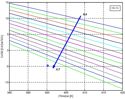
By considering the three domaintating parameters including: the auto ignition level, amount of injected fuel in the premixed mixture and the mixture temperature at the IVC moment (after mixing with the resual gas)], the MKIM integral can be condensed into a map predicting SOC as a function of the mentioned parameters.This is easier to handle than any explicit analytical expression for MKIM:
(3)
where, ON is the octane number of the dual fuel mixture and k, is the cycle number subscript.
2. 2. Combustion Duration
In [14], a modified Weib function was parameterized and used in order to predict the combustion duration. As a simplification, in an operating range, the burn duration can be considered constant.The cranke angle at which 50% of the fel is burnt is a robust feedback signal for HCCI combustion control [14]. Due to this simplification, CA50 and the end of the combustion (EOC) can be obtained by Eq.s (4) and (5):
(4)
(5)
Where is the combustion duration. Eventually, the SOC map turns into a CA50 map (Fig.1). According to the derived maps, by having the mixture temperature at IVC point, fuel equivalence ratio and the fuel mixture octane number, the combustion timing can be predictable.
2. 3. The Role of the Residual Gas in the Dynamic Cyclic Coupling
At the end of each cycle, a fraction of the combustion gases, called residual gas, is trapped in cylinder after the exhaust valve closure (EVC) moment. This residual gas is mixed with the fresh air-fuel charge of the next cycle and has heating and dilution effects on it [14]. This phenomenon dynamically couples each two consecutive engine cycles. Therefore it is important to determine the mass amount and the temperature of the residual gas, since both of these factors are important in determining the next cycle mixture temperature at IVC moment. It is needed to track the stages from SOC to EVC until the required parameters are achieved.
2. 3. 1. Combustion Temperature Increase
In the previous work [14], the engine cylinder was considered as a closed system between SOC and EOC and by considering the first law of thermodynamics, the temperature at the end of the combustion was found. As a simplification, by neglecting the heat transfer to the cylinder wall, the temperature increase due to the combustion process can be obtained by Eq. (6) [15].
(6)
Where mfuel is the mass of injected fuel in the premixed mixture and mt is the total mass of the combustion mixture. CoC and are the completeness of combustion coefficient and the specific heat capacity of the mixture, respectively which are both considered as average constant values.
ܥҧ௩ ȟܶǡାଵൌ
݉௨ǡ ܮܪܸ௨ܥܥ ݉௧ǡାଵ ܥҧ௩
οߠ
ܧܱܥାଵൌ ܱܵܥାଵ οߠ
ܥܣͷͲାଵൌ ܱܵܥାଵଵଶοߠ
ܱܵܥାଵൌ ܨ ൫ሺܶ௩ሻ௫ǡାଵǡ ܱܰǡ Þ൯
390 395 400 405 410 415 420
-10 -5 0 5 10 15
(Tmix)ivc [K]
CA
50
[C
A
D
aT
DC
]
ON=10
0.7
0.4
ø
Fig. 1.CA50 map (at ON=10)
The fuel mixture heating value (LHVfuel)can be estimated as a function of the volume percentage, density and the heating value of each of the PRFs [14] The total mass of the combustion mixture consists of the mass of fuel, air and the residual gas, also, the equivalenec ratio is the fraction of the actual fuel-air ratio to the stoichiometric fuel-air ratio and finally the residual gas fraction is the ratio of the trapped residal gas to the mass of the total inducted air-fuel mixture. By considering the mentioned definitions, Eq. (6) turns into Eq. (7):
(7)
Where AFRst is the stoichiometric air-fuel ratio, RGF is the residual gas fraction and is the average heating capacity of the combustion mixture. Hence, the temperature at EOC moment is obtained by Eq. (8):
(8)
The pressure at EOC is obtained by assuming the mass conservation law for the cylinder as a closed system (between SOC and EOC) along with the ideal gas state Eq.s [14].
Similar to the compression process, a polytropic expansion can be considered for the expansion of the burned gas, moreover, as a simplification, the exhaust process is considered polytropic, while assuming the exhaust manifold pressure at the atmosphere value, therefore, the temperature at EVC moment or the residual gas temperature, can be obtained by Eq. (9):
(9)
The residual gas fraction is defined as the mass ratio of the residual gas to the inducted air-fuel mixture:
(10)
where, RGF is the residual gas fraction and mevcis the mass of the trapped residual gas, obtained by the ideal gas Eq. at EVC moment. minitial is the mass of the initial inducted air-fuel mixture that can be obtained by the ideal gas equation (PV=M T ), at each definite point before EVO (for instance at EOC). Therefore Eq. (10) turns into:
(11)
Where is the gas average constant value. The obtained residual gas fraction and temperature affect the inducted air-fuel mixture temperature at the subsequent cycle at its IVC moment and hence, the two subsequent cycles are thermally coupled.
3. MODEL STATES AND DISTURBANCES Combustion timing (CA50) and the temperature increase due to the combustion are considered as the control model states. The combustion temperature increase has importance since it dominates the temperature of the residual gas which affects the next cycle intake charge temperature. On the other hand, the intake charge properties affect the combustion timing and hence, the intake temperature Tmanpressure Pmanand the fuel equivalence ratio are considered as the disturbances.
By stepping through the above mentioned processes, the residual gas fraction and temperature is derived as functions of the model states (CA50 and T) and therefore link the states of the two consecutive cycles. For two successive cycles: kand k+1, the model state space and output equations are achievable:
(12)
(13)
where, the disturbance vector (W) is shown in (14):
(14)
4. MODEL VALIDATION
It is necessary to show that the developed simplified control model can predict its combustion timing with a proper level of accuracy. Therefore, this control model should be validated against the transient experimental results for the same control input variation.
As it can be seen in Fig. 2, the model is validated against the experimental results from [14] for a transient octane number input experiment. The
ܹ
ൌ ൣ
ǡ ܶ
ǡǡ ܲ
ǡ൧
்ȟܶାଵൌ ܨଶሺܥܣͷͲǡ ȟܶǡ ܱܰǡ ܹሻ ܥܣͷͲାଵൌ ܨଵሺܥܣͷͲǡ ȟܶǡ ܱܰǡ ܹሻ
¨ ܴത
ܴܩܨାଵൌ
ೌ
ǡೖశభ
ೡ
ǡೖశభ
்ǡೖశభ
்ೃಸǡೖశభ
ோത
ோതೡ
ܴത
ܴܩܨାଵൌ
݉௩ǡାଵ
݉௧ǡାଵ
ܶோீǡାଵൌ ܶǡାଵ ൬ ೡǡೖశభ൰
ିଵ
ܶǡାଵൌ ܶ௦ǡାଵ ȟܶǡାଵ ܥҧ௩ ȟܶǡାଵൌ
ܮܪܸ௨ܥܥ
ሺͳ ܴܩܨሻ ቀܣܨܴ௦௧ ͳቁ ܥҧ௩
specifications of the engine is shown in Table 1. Furthermore, according to Fig. 2, the control model is compared with the simulation results of the previously introduced physical model [14].
As it can be seen, the nonlinear control model can suitably capture the engine operation under the transient ON input with an uncertainty (standard deviation) of about ± 1.8 CAD with the average error of 1.8 CAD.
5. MODEL LINEARIZATION
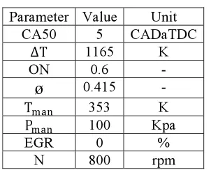
The nonlinear state space model is linearized around a nominal operating point and the first term of Taylor series is derived. The engine operational parameters at this point are shown in Table 2.
In order to have a more detailed view of the effects of the parameters on the combustion timing, the operational parameters are defined in form of the normalized deviation from their values at the nominal operating point (15):
(15)
where, q can be model states, input, output or the physical disturbances. By substituting these parameters as functions of their normalized deviation forms, the linear state space and output equations are obtained as shown in Eq. (16) and (17):
(16)
ܺ෨ାଵൌ ܣሚܺ෨ ܤ෨ݑ ܨ෨ܹ෩
ݍ ൌିതത
0 50 100 150 200 250 300 350 400 445
0 10 20
CA
5
0
[C
A
D
a
T
D
C
]
0 50 100 150 200 250 300 350 400 445
0 10 20 30
ON
0 50 100 150 200 250 300 350 400 445
0.4 0.42 0.44
Ø
0 50 100 150 200 250 300 350 400 445
810 815 820
Cycle No.
N [
rp
m
]
Simplified Control Model Physics Based Model Exp.
Fig. 2. Transient validation of the nonlinear control model
Unit Value
Parameter
mm 80
Bore
mm 88.90
Stroke
-10
Compression Ratio
Liter 0.447
Displacement Volume
4 Number of
Valves
CADaBDC -175/+55
IVO/IVC
CADaBDC -70/-175
EVO/EVC
Table 1.The Specifications of the single cylinder Ricardo engine
Parameter Value Unit
CA50 5 CADaTDC
ȟ 1165 K
ON 0.6 -
ø
0.415୫ୟ୬ 353 K
୫ୟ୬ 100 Kpa
EGR 0 % N 800 rpm
Table 2.Operating point around which the nonlinear model is linearized
(17)
Where and are the normalized state and the normalized disturbance vectors, respectively. Meanwhile, and are the normalized input and output scalars. The matrices that define this operating condition are shown in (18):
(18)
The values of these matrices’ elements are directly linked to the values of the operational engine parameters at the selected nominal operating point.
6. CONTROL DESIGN
6. 1. Optimal Integral State-Feedback Control According to the linearized model derived in Section 5, a state feedback controller is considered along with an integral controller in order to compensate any probable steady state error and also non-robustness of the state feedback control. The control design is conducted for non normalized matrices. By adding the integral controller, the model order increases by a unit and the augmented model state space equation is found:
(19)
Where X is the model state vector and XIis the integral state. The control signal can be obtained by Eq. (20):
(20)
Where KIis the integral controller gain and K is the state feedback gain vector. The matrices for the augmented model equations along with the state and control gain vectors are shown in (21):
(21)
where the subscript:”aug”, refers to augmented model.
The values of the control gains directly affect the control performance indices such as control speed and the overshoot or undershoot values [20].
Optimization can be a suitable method to obtain the gains in order to have the most desirable condition for the control performance indices. Hence, linear quadratic optimization (LQ) is used for the augmented model in order to find the optimal control gains. The gains should be chosen in a way that minimizes the performance index in (22).
(22)
where, the control signal is derived by Eq. (20). The control gain vector (kaug) can be obtained by Eq. (23):
(23)
Matrix P is derived by solving Riccati equation in (24):
(24)
where, Q is a symmetric positive semi-definite matrix and R is a positive definite scalar:
(25)
Weighting matrices Q and R highly affect the values of the control gains and hence, the performance of the controller. Finding the optimal values for these weighting matrices can be the solution to satisfy the control criteria.
6. 2. GA Optimal Determination of the State Feedback Weighting Matrices
There have been different methods including optimal methods [21] and non-optimal trial and error for selecting the state feedback weighting matrices. In each nontrivial engineering problem with a number of objectives, one of the efficient ways to find the best solutions is using multi
ܳ ൌ ሾܳଵǡଵ Ͳ
Ͳ Ͳሿ
ܲ ൌ ܳ ܣ௨்ܲ൫ܫ ܤ௨ܴିଵܤ௨்ܲ൯ିଵܣ௨ ܭ௨ൌ ൫ܴ ܤ௨்ܲܤ௨൯
ିଵ ܤ்ܲܣ
௨
ܥ௨ൌ ܥ ܭ௨ൌ ሾܭூ ܭሿ ܺ௨ൌ ቂ
ݔூ ܺቃ ܣ௨ൌ ቂͳ ܥͲ ܣቃ ܤ௨ൌ ቂͲ
ܤቃ
ݑൌ െሾܭூ ܭሿ ቂ
ݔூ
ܺቃ
ቂݔܺூቃ
ሺାଵሻൌ ቂ ͳ ܥ
Ͳ ܣቃ ቂ
ݔூ ܺቃ ቂ
Ͳ ܤቃݑ
ܣሚ ൌ ቂെͲǤͲʹͺ െͲǤͺͲͷ͵ ͲǤͲͲͳͳ ͲǤͲ͵ʹʹቃ
ܤ෨ ൌ ቂͲǤͲ͵͵
Ͳ ቃ ܿǁ ൌ ሾͳ Ͳሿ
ܨ෨ ൌ ቂെͲǤͲʹʹ െͲǤͲͲͳ െͲǤͲͲͳʹ
ͲǤͲͲͲ Ͳ Ͳ ቃ
ݕ ݑ
ܹ෩
ܺ෨
ݕൌ ܿǁܺ෨objective methods. In this study, this method can be exploited in order to find the solutions convincing all the control performance indices, relatively.
Multi objective genetic algorithm is an evolutionary optimization algorithm [22] which has been used for finding the optimal solutions in order to minimize or maximize multi objective functions. An important advantage of this algorithm is that instead of finding a particular solution to a single objective which can result in undesirable consequences in relation to other objectives, a set of solutions is obtained. Each of these solutions satisfies all the objectives at an acceptable level without any domination by any other solution.
In this paper, a method called NSGAII [23], is used to find the optimal solutions. This method is a pareto based method. Pareto optimal solution is the solution that is not dominated by any other solution in the solution space. The corresponding objective functions to these solutions are called: “pareto front”.
Three distinguished control indices are chosen as the objective functions: Maximum Overshoot (MOS) as the maximum deviation from the steady state output value, settling time (ST) as the first time at which the output CA50 reaches the range of 5 % around the steady state value and finally, rise time, (RT) as the first time at which the controlled plant CA50 reaches the desired steady state value.
Since simulating the control structure model (including the plant and controller) is too
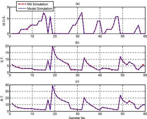
time-consuming, an artificial neural network is designed to be trained for efficient prediction of the control performance criteria in response to the given values of the weighting matrices. The developed neural network has two hidden layers, each of which has 20 nodes. The input layer has two nodes (Q1,1and R) and the control performance indices constitute the three output nodes. The structure of this neural network is shown in Fig. 3.
The model is simulated for a wide range of Q1,1and R variations from 0.02 to 10 and from 0.02 to 2, respectively. 50 % of the simulation results are used for training the neural network, while the rest of the data are used for testing and validating the neural network performance (Fig. 4).
According to the validation results, the developed neural network seems to be promising in predicting the
Fig. 3.Neural network structure
0 10 20 30 40 50 60
0 5 9
M.O
.S
.
(a)
0 10 20 30 40 50 60
0 5 10 15 20
S.
T.
(b)
0 10 20 30 40 50 60
0 10 20 30 40
Sample No.
R.
T
.
(c) NN Simulation
Model Simulation
Fig. 4.NN validation: (a): M.O.S, (b): S.T., (c): R.T.
control performance as a function of the controller weighting matrices. This neural network is coupled with multi objective genetic algorithm method in order to find the pareto optimal-set [22]. The corresponding objective functions or pareto fronts (control performance indices) are found. These pareto fronts give an interesting flexibility to designers to put an emphasis on one or two particular objectives and select their desirable solution among the pareto optimal-set. According to the obtained optimal-set, the desired weighting matrices are selected that are shown in (26).
(26)
The linear quadratic optimization is implemented on the augmented model (Eq. (22) to (24)) which leads to the following control gains:
(27)
6. 3. State Observer Design
Since at least one of our states is not easily measurable, it is needed to design and use a state observer to estimate the states [20]. The observer equations are shown in Eq. (28) and (29).
(28)
(29)
Where and are the observed state vector and output, respectively and l is the Luenberger gain vector.
7. RESULTS AND DISCUSSION 7. 1. Controller Tracking Performance
The performance of the designed optimal integral state feedback controller is investigated by implementation on the more complex physical model from [14] (Fig. 5). Also, the values of the tracking performance indices are shown in Table 3. The performance of the state observer during this transient operation is shown in Fig. 6.
As can be seen, not only the trends of variations are the same for both the simulated and estimated states, but also there is a suitable accuracy in this estimation with an average error of about 6 Kelvin degrees for the temperature increase estimation.
ݕො ܺ ݕොൌ ܥ ܺ
ܺାଵൌ ܣ ܺ ܤݑ ݈ ሼݕെ ݕොሽ ܨ ܹ
ܭூൌ ʹǤͳͷͻܭ ൌ ሾʹǤͷͶͷ െͲǤͲͲͻʹሿ
ܳ ൌ ሾʹǤͲͻ͵ʹ Ͳ
Ͳ Ͳሿ, R= 0.0442
0 10 20 30 40 50 60 70 80 90 100 4
5 6 7 8 9
C
A5
0
[C
AD
a
T
DC
]
0 10 20 30 40 50 60 70 80 90 100 5
10 15
0
Cycle No.
ON
I+SFC Desired
Fig. 5.Tracking performance of the optimal integral state feedback controller
Control Performance Index Value Unit
Rise Time 3 engine cycle
Settling Time 2 engine cycle
Maximum Overshoot 4 percentage
Steady-state Error 0 percentage
Fig. 6.Estimation of States
Table 3.Control performance for tracking from CA50= 5 to 7 CADaTDC
0 10 20 30 40 50 60 70 80 90 100
4 5 6 7 8 9
CA
5
0
[CAD
a
T
D
C
]
0 10 20 30 40 50 60 70 80 90 100
950 1000 1050 1100
Cycle No.
T
e
mp
. In
cr
e
a
se
[K
]
Plant State Observed State
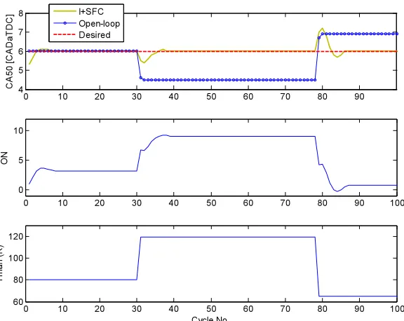
7. 2. Robustness to the Variations of the Intake Charge Properties
HCCI combustion is sensitive to some physical parameters specially intake charge characteristics [2,3] including the intake temperature, pressure and the equivalence ratio in the premixed inducted
mixture. So, it is important for an efficient HCCI controller to keep the engine stability under such sort of physical disturbances. In Fig. 7-9, the robustness of the controller is studied under the variations of the equivalence ratio and the intake pressure (load disturbances) and the intake temperature, respectively.
As can be seen, the designed controller can
0 10 20 30 40 50 60 70 80 90 100
4 5 6 7 8
CA
5
0
[C
AD
a
T
DC]
0 10 20 30 40 50 60 70 80 90 100
0 5 10
ON
0 10 20 30 40 50 60 70 80 90 100
0.4 0.42 0.44
Cycle No.
Ø
I+SFC Open-loop Desired
Fig. 7.Rejecting the external disturbance of equivalence ratio
0 10 20 30 40 50 60 70 80 90 100
2 4 6 8
C
A
50 [
C
A
D
aT
D
C
]
0 10 20 30 40 50 60 70 80 90 100
0 2 4 6 8
ON
0 10 20 30 40 50 60 70 80 90 100
90 100 110 120
Cycle No.
P
m
a
n
[K
P
a
]
I+SFC Desired Open-loop
Fig. 8.Rejecting the external disturbance of the intake pressure
effectively reject the physical disturbances and keep the engine combustion timing (CA50) in its desirable range, which is between 5 to 8 CADaTDC due to low level of cyclic variation [24].
For the equivalence ratio variation, while the CA50 of the open loop model is deviated by about 20%, the controller keeps the closed loop output in the region around 10% of the desired steady value. Reaching the steady value needs a time period of 4 cycles. For the intake pressure disturbance, the 25% deviation of the open loop model is compensated to 10% and a period of 3 cycles is needed to make the error vanish. Finally, for the intake temperature variation, the controller compensates the 25 % deviation of the open loop response to only 6% and makes the model reach the desired steady CA50 value within 5 cycles.
8. CONCLUSION
A simplified model for control of HCCI combustion timing was introduced. The model was validated against both experimental data and results from a detailed physics-based HCCI model. The states and disturbances were chosen in a way to widely include the main influential factors affecting HCCI combustion timing. An optimal integral state feedback combustion timing controller was designed to track the desired combustion timing by adjusting the fueling mixture ratio. Apart from suitable tracking
performance, the controller exhibited desirable disturbance rejection characteristic under variation of the external physical intake disturbances such as the fuel equivalence ratio, temperature and pressure. The controller has kept the engine operation in its desired range and rejected the disturbances with relatively high speed with an order of 3 to 4 cycles.
REFERENCES
[1] F. Zhao, T. W. Asmus, D. N. Assanis, J. E. Dec, J. A. Eng, and P. M.Najt, “Homogeneous Charge Compression Ignition (HCCI) Engines”, SAE Publication PT-94, 2003. [2] M.Shahbakhti ,”Modeling and Experimental
Study of an HCCI Engine for Combustion Timing Control”, PHD. Thesis, University of Alberta, 2009.
[3] J. Bengtsson, P. Strandh, R. Johansson, P. Tunest°al, and B. Johansson, “Hybrid Modeling of Homogeneous Charge Compression Ignition(HCCI) Engine Dynamic—A Survey,” Int. J. of Control, vol. 80, No. 11, pp. 1814–1848, Nov. 2007.
[4] J. O. Olsson, P. Tunestºal, and B. Johansson,”Closed-Loop Control of an HCCI Engine”,SAE Paper No. 2001-01-1031, 2001. [5] P. Strandh, J. Bengtsson, R. Johansson, P.
Tunesta, and B. Johansson, “Variable Valve
0 10 20 30 40 50 60 70 80 90
4 5 6 7 8
C
A
50 [
C
A
D
aT
D
C
]
0 10 20 30 40 50 60 70 80 90 100
0 5 10
ON
0 10 20 30 40 50 60 70 80 90 100
60 80 100 120
Cycle No.
Tm
an
(
K
)
I+SFC Open-loop Desired
Fig. 9.Rejecting the external disturbance of the intake temperature
Actuation for Timing Control of a HCCI Engine ", SAE Paper No. 2005-01-0147, 2005. [6] G. Haraldsson, P. Tunestºal, B. Johansson, and J.
HyvÄonen, “HCCI Closed- Loop Combustion Control Using Fast Thermal Management”, SAE Paper No. 2004-01-0943, 2004.
[7] R. Pfeiffer, G. Haraldsson, J-O Olsson, P. Tunestºal, R. Johansson and B. Johansson, “System Identification and LQG Control of Variable-Compression HCCI Engine Dynamics”, Proceeding of the 2004 IEEE, International conference on Control Applications, Taipei, Taiwan, September 2-4, 2004.
[8] D. Law, D. Kemp, J. Allen, G. Kirkpatrick, and T. Copland, “Controlled Combustion in an IC-Engine with a Fully Variable Valve Train”, SAE Paper No. 2000-01-0251, 2000.
[9] G. M. Shaver, M. J. Roelle, and J. C. Gerdes, “Modeling Cycle to Cycle Dynamics and Mode Transition in HCCI Engines with Variable Valve Actuation”, Journal of Control Engineering Practice, vol. 14, pp. 213-222, 2006.
[10] F. Agrell, H-E. Ångström, B. Eriksson, J. Wikander and J. Linderyd, “Integrated Simulation and Engine Test of Closed Loop HCCI Control by aid of Variable Valve Timings”, SAE Paper No. 2003-01-0748, 2003. [11] G. M. Shaver, J. C. Gerdes, and M. J. Roelle,” Physics Based Closed-loop Control of Phasing, Peak pressure and work output in HCCI Engines utilizing Variable Valve Actuation”, In Proceedings of the American Control Conference, pp. 150-155, Boston, Massachusetts, 2004.
[12] C. J. Chiang and C-L. Chen, “Constrained Control of Homogeneous Charge Compression Ignition (HCCI) Engines”, 2010 5th IEEE Conference on Industrial Electronics and Applications, pp. 2181-2186, 2010.
[13] C. J. Chiang, C-C. Huang and M. Jankovic, “Discrete-time Cross-term Forwarding Design of Robust Controllers for HCCI Engines”, 2010 American Control Conference, ”, pp. 2218-2223, Marriott Waterfront, Baltimore, MD, USA, June 30-July 02, 2010.
[14] M. Shahbakhti and C.R. Koch, “Physics Based Control Oriented Model for HCCI Combustion Timing”, Journal of Dynamic Systems,
Measurement and Control, vol. 132, pp.1-58, 2010.
[15] J. B. Heywood, Internal Combustion Engine Fundamentals, McGraw Hill, New York,1988. [16] M. Halstead, L. Kirsch, and C. Quinn, “The
Auto Ignition of Hydrocarbon Fuels at High Temperatures and Pressures — Fitting of a Mathematical Model”, Combustion and Flame, vol.30, pp. 45–60, 1977.
[17] S. R. Turns,”An Introduction to Combustion: Concepts and Applications”, McGrawHill series in mechanical engineering, McGraw-Hill, 2nd edition, 2000.
[18] J. C. Livengoodand P. C.Wu,”Correlation of Autoignition Phenomena inInternalCombustion Engines and Rapid Compression Machines”, Fifth Symposium (International) on Combustion, 1955.
[19] M. Shahbakhti, C. R. Koch, “Thermo-kinetic Combustion Modeling of an HCCI Engine to Analyze Ignition Timing for Control Applications “, Proceeding of Combustion Institute-Canadian Section (CICS) Spring Technical Conference, 6 pages, May 13-16, 2007, Banff, Canada, 2007.
[20] F .F. Franklin, J. D. Powell, and M. Workman, Digital Control of Dynamic Systems, Addison Wesley, 1998.
[21] Y. Li, J. Liu and Y. Wang, “Design approach of weighting matrices for LQR based on multi-objective evolution algorithm”, International Conference on information and Automation, Changsha, 2008.
[22] A. H. F. Dias and J. A. de Vasconcelos ,” Multiobjective Genetic Algorithms Applied to Solve Optimization Problems”, IEEE Transactions on Magnetics,, vol. 38, No. 2, pp.1133-1136, 2002.
[23] K. Deb, S. Agrawal, A. Pratap and T. Meyarivan,” A Fast and Elitist Multiobjective Genetic Algorithm: NSGA-II”, IEEE Transactions on Evolutionary Computation, vol. 6, pp.182-197, 2002.
[24] M. Shahbakhti, R. Lupul, and C. R. Koch, “Cyclic Variations of Ignition Timing in an HCCI Engine", Proceeding of ASME/IEEE Joint Rail Conference & Internal Combustion Engine Spring Technical Conference, 2007.
List of Symbols
= average constant volume specific heating capacity
CA50= crank angle for 50% burnt fuel (CAD aTDC) CADaBDC= crank angle degree after bottom dead
centre
CADaTDC= crank angle degree after top dead centre = average completeness of combustion T= temperature increase due to the combustion
process (K)
EGR= exhaust gas recirculation EOC= end of combustion (CAD aTDC) GA = genetic algorithm
LHV= lower heating value NN= neural network RGF = residual gas fraction
SOC= start of combustion (CAD aTDC)
Subscripts aug= augmented eoc= end of combustion evc= exhaust valve closure ivc=intake valve closure man= manifold
mix= mixture RG= residual gas soc= start of combustion
(
ሻ
¨
തതതതത
(
) ܥҧ௩