in the population sciences published by the Max Planck Institute for Demographic Research Konrad-Zuse Str. 1, D-18057 Rostock·GERMANY www.demographic-research.org
DEMOGRAPHIC RESEARCH
VOLUME 18, ARTICLE 3, PAGES 59–116
PUBLISHED 12 MARCH 2008
http://www.demographic-research.org/Volumes/Vol18/3/ DOI: 10.4054/DemRes.2008.18.3
Research Article
Perturbation analysis of nonlinear matrix
population models
Hal Caswell
c
°2008 Caswell.
1 Introduction 60
2 Matrix calculus 64
3 Density-dependent models 66
4 Environmental feedback models 72
5 Subsidized populations and competition for space 74
6 Sensitivity of proportional age and stage distributions 82
7 Frequency-dependent two-sex models 89
8 Sensitivity of population cycles 94
9 Sensitivity of life expectancy 103
10 Summary and discussion 106
11 Acknowledgments 107
Perturbation analysis of nonlinear matrix
population models
Hal Caswell1,2
Abstract
Perturbation analysis examines the response of a model to changes in its parameters. It is commonly applied to population growth rates calculated from linear models, but there has been no general approach to the analysis of nonlinear models. Nonlinearities in de-mographic models may arise due to density-dependence, frequency-dependence (in 2-sex models), feedback through the environment or the economy, and recruitment subsidy due to immigration, or from the scaling inherent in calculations of proportional population structure. This paper uses matrix calculus to derive the sensitivity and elasticity of equi-libria, cycles, ratios (e.g., dependency ratios), age averages and variances, temporal aver-ages and variances, life expectancies, and population growth rates, for both age-classified and stage-classified models. Examples are presented, applying the results to both human and non-human populations.
1Distinguished Research Scholar, Max Planck Institute for Demographic Research
2Senior Scientist, Biology Department MS-34, Woods Hole Oceanographic Institution, Woods Hole MA
1. Introduction
The goal of this paper is to present a new approach to the perturbation analysis of nonlin-ear population models, providing the sensitivity and elasticity of a wide range of demo-graphic quantities.
1.1 Perturbation analysis
The output of any model depends on the values of its parameters. Perturbation analysis asks how changes in one or more parameters will affect the output. Widely used by de-mographers of all types, perturbation analysis is important in evolutionary biology (where the perturbations are produced by mutation or recombination), conservation, pest control, and and population policy (where the concern is with management manipulations), and sampling theory (the parameters to which a quantity is most sensitive are those that must be estimated most precisely). The results of perturbation analysis are often expressed as sensitivities (the sensitivity ofytoxis the derivativedy/dx) and elasticities (the elasticity ofytoxis(x/y)dy/dx).
The perturbation analysis of linear demographic models has focused on the sensitivity ofλorr(e.g., Keyfitz 1971, Hamilton 1966, Caswell 1978, Baudisch 2005), of the stable age or stage distribution (Coale 1957, 1972, Caswell 1982), and of life expectancy (Key-fitz 1977, Pollard 1982, Vaupel 1986, Vaupel and Romo 2003, Caswell 2006). The per-turbation analysis of short-term transient dynamics has recently been presented (Caswell 2007a).
This paper presents new methods for perturbation analysis of nonlinear models, using matrix calculus. It uses those methods to analyze the sensitivity of a selection of important
nonlinearmodels: density-dependent, environment-dependent, subsidized, two-sex, and
proportional structure models.
Plant and animal demographers have recognized the need for sensitivity analysis of nonlinear models (e.g., Grant and Benton 2000, 2003), but until now there has been no general perturbation analysis for such models. Instead, most studies have relied on nu-merical calculations using difference quotients. This is a notoriously unstable method for computing derivatives, requires lots of computation, and provides no analytical insight into the structure of the sensitivities.
together with a measure of genetic variation it determines the rate of phenotypic change under selection. The sensitivity of the invasion exponent to parameter changes has been shown to be equal to the sensitivity of a kind of weighted average population density to those parameter changes (Takada and Nakajima 1992, 1998, Caswell et al. 2004, Caswell 2007b).
1.2 Organization of this paper
Because this paper relies on techniques from matrix calculus, I begin in Section 2. with a brief review of those techniques. Section 3. analyzes density-dependent models, in-troduces methods for analyzing various dependent variables, and shows how to calculate elasticities as well as sensitivities. Sections 2. and 3. are essential to the rest of the paper. The subsequent sections can, to an extent, be read independently. Section 4. analyzes environmental feedback models, Section 5. analyzes subsidized models and Section 6. considers the equilibria of proportional structures, such as arise in calculating the stable stage distribution, the dependency ratio, and means and variances of age at reproduction. Section 7. analyzes frequency-dependent two-sex models, including the sensitivity of both population structure (Section 7.1) and growth rate (Section 7.2). Finally, Section 8.1 an-alyzes the sensitivity of cycles in density-dependent models. For a preview of the results that will be in hand by the end of the paper, skip ahead to Table 3.
This paper contains examples from animal, plant, and human populations, because I assume at the outset that demographic studies on different species have the potential to inform each other, especially if the species differ in interesting biological properties. This perspective has a long history (e.g., Pearl et al. 1927) and enough recent examples (e.g., Wachter and Finch 1997, Carey 2003, Wachter and Bulatao 2003, Keyfitz and Caswell 2005) that it is now referred to as biodemography (Carey and Vaupel 2005).
1.3 Nonlinear models and their dynamics
Nonlinearity is defined in contrast to linearity. Ifxis an age or stage distribution vector, and if the dynamics ofxare
x(t+ 1) =f[x(t)], (1)
then the model is linear iff(·)is a linear function, i.e., if
f(ax1+bx2) =af(x1) +bf(x2) (2)
for any constantsaandband any vectorsx1andx2.
Density-dependence: arises when the per-capita vital rates are functions of the numbers or density of the population. Such effects are well documented in plants (e.g., Sol-brig et al. 1988, Gillman et al. 1993, Silva Matos et al. 1999) and animals (e.g., Pennycuick 1969, Longstaff 1977, Clutton-Brock et al. 1997, Tanner 1999, Cush-ing et al. 2003). Density-dependence has been intensively studied in the laboratory (e.g., Pearl et al. 1927, Frank et al. 1957, Costantino and Desharnais 1991, Carey et al. 1995, Mueller and Joshi 2000, Cushing et al. 2003). It can arise from com-petition for food, space, or other resources, or from interactions (e.g., cannibalism) among individuals.
Simple density-dependence is less often invoked by human demographers.3 Weiss
and Smouse (1976) proposed a density-dependent matrix model, and Wood and Smouse (1982) applied it to a population of the Gainj people of Papua New Guinea. Density-dependence is included in epidemiological feedback models applied to a rural English population in the 16th and 17th centuries by Scott and Duncan (1998). The Easterlin effect (e.g., Easterlin 1961) produces density-dependence in which fertility is a function of cohort size. Analysis of the Easterlin effect has focused mostly on the possibility that it could generate cycles in births (e.g., Lee 1974, 1976, Frauenthal and Swick 1983, Wachter and Lee 1989, Chu 1998).
Environmental (or economic) feedback. Density-dependent models are often an attempt to sneak in, by the back door as it were, a feedback through the environment. A change in population size changes some aspect of the environment, which af-fects the vital rates, which in turn affect future population size. MacArthur (1972) showed that simple density-dependent models in ecology could be derived from to models including the feedback between the dynamics of consumers and their re-sources. Consumer-resource models (e.g., Hsu et al. 1977, Tilman 1982, Murdoch et al. 2003) are the basis for the models of food chains and food webs that underlie models of global biogeochemistry (Fennel and Neumann 2004).
Feedback models are often invoked in human demography, with the feedback op-erating through the economy (Lee 1986, 1987, Chu 1998). An interesting aspect of these approaches is the possibility that, if larger populations support more robust economies, the feedback could be positive instead of negative (Lee 1986, Cohen 1995, Appendix 6). An exciting combination of ecological and economic feedback appears in the food ratio model recently proposed by Lee and Tuljapurkar (2007).
3Lee (1987) reviewed the situation and said “. . . we might say that human demography is all about Leslie
Two-sex models. To the extent that both males and females are required for reproduction (and, in the bigger scheme of things, this is not always so), demography is nonlinear because the marriage function or mating function cannot satisfy (2). Nonlinear two-sex models have a long tradition in human demography (see reviews in Keyfitz 1972b, Pollard 1977) and have been applied in ecology (e.g., Lindström and Kokko 1998, Legendre et al. 1999, Kokko and Rankin 2006, Lenz et al. 2007). Their mathematical properties have been investigated by e.g, Caswell and Weeks (1986), Chung (1994), Ianelli et al. (2005), and in a very abstract setting by Nussbaum (1988, 1989).
In their most basic form, two-sex models differ from density-dependent models in that the vital rates depend only on the relative, not the absolute, abundances of stages in the population (they are sometimes called frequency-dependent for this reason). This has important implications for their dynamics.
Models for proportional population structure. Even when the dynamics of abundance are linear, the dynamics of proportionalpopulation structure are nonlinear (e.g., Tuljapurkar 1997). This leads to some useful results on the sensitivity of the stable age or stage distribution and the reproductive value.
Linear models lead to exponential growth and convergence to a stable structure. Much of the analysis of linear models focuses on the population growth rateλor r = logλ. Nonlinear models do not usually lead to exponential growth (frequency-dependent two-sex models are an exception). Instead, their trajectories converge to an attractor. The attractor may be an equilibrium point, a cycle, an invariant loop (yielding quasiperi-odic dynamics), or a strange attractor (yielding chaotic dynamics); see Cushing (1998) or Caswell (2001, Chapter 16) for a detailed discussion.
In this paper, I will analyze the sensitivity and elasticity of equilibria and cycles. Be-cause the dynamic models considered here are discrete, solutions always exist and are unique. The nature of number of the attractors depends on the specific model. Perturba-tion analysis always considers perturbaPerturba-tions ofsomething, so the equilibria or cycles must be found before their perturbation properties can be analyzed.
A note on notation. Matrices are denoted by upper case bold symbols (e.g.,A), vectors (usually) by lower case bold symbols (n);aijis the(i, j)entry of the matrixA,niis the ith entry of the vectorn, andnTis the transpose ofn. The exceptions to these conventions are noted when they occur. Logarithms are natural. The vector normkxkis, unless noted otherwise, the 1-norm. In addition to the ordinary matrix product, the Kronecker product
matrix isI; sometimes its dimension will be indicated by a subscript, as inIsfor thes×s
identity. The end of an example is denoted by the symbol♦.
2. Matrix calculus
Matrix calculus permits the consistent differentiation of scalar-, vector-, and matrix-valued functions of scalar, vector, or matrix arguments. Because this method is not well-known in either ecology (but see Caswell 2006, 2007a) or demography (but see Willekens 1977, Ekamper and Keilman 1993 for related approaches), the next section presents a brief statement of the essential results. More detail can be found in Caswell (2007a). There exist several conventions for matrix calculus, differing in their arrangements of the matrix and vector entries. The best is that of Magnus and Neudecker (1985, 1988); it is called the vector-rearrangement method in the review paper of Nel (1980).
Ifxandyare scalars, the derivative ofy with respect toxis the familiar derivative
dy/dx. Ifyis an×1vector andxa scalar, the derivative ofywith respect toxis the
n×1vector
dy
dx =
dy1
dx
.. .
dyn dx
. (3)
Ifyis a scalar andxis am×1vector, the derivative ofywith respect toxis the1×m
gradient vector
dy dxT =
µ ∂y ∂x1
· · · ∂y
∂xm
(4)
Note the orientation ofdy/dxas a column vector anddy/dxTas a row vector.
Ifyis an×1vector andxam×1vector, the derivative ofywith respect toxis the
n×mJacobian matrix
dy
dxT = µ
dyi dxj
. (5)
Derivatives involving matrices are written by transforming the matrices into vectors using the vec operator (which stacks the columns of the matrix into a column vector), and then applying the rules for vector differentiation. Thus, the derivative of them×nmatrix
Ywith respect to thep×qmatrixXis themn×pqmatrix
dvecY
dvecTX
For notational convenience, I will write vecTXfor(vecX)T.
These definitions (unlike some alternatives; see Magnus and Neudecker 1985) lead to the familiar chain rule. IfYis a function ofXandXis a function ofZ, then
dvecY
dvecTZ =
dvecY
dvecTX
dvecX
dvecTZ. (7)
The derivatives of matrices are constructed by forming the differentials of the expres-sions involving the matrices. The differential of a matrix (or vector) is the matrix (or vector) of differentials of the elements; i.e.,
dX=¡ dxij ¢
. (8)
If, for vectorsxandyand some matrixQ, it can be shown that
dy=Qdx (9)
then
dy
dxT =Q. (10)
(the “first identification theorem” of Magnus and Neudecker (1985); see also Neudecker 1969).
The combination of the chain rule and the identification theorem permits more com-plicated expressions involving differentials to be turned into derivatives with respect to an arbitrary vector, sayu. If
dy=Qdx+Rdz (11)
then
dy
duT =Q
dx
duT+R dz
duT (12)
for anyu.
We will make extensive use the Kronecker product, defined as
A⊗B=
a11B a12B · · ·
a21B a22B · · ·
..
. ... . ..
. (13)
The vec operator and the Kronecker product are related (Roth 1934); if
Y=ABC (14)
then
3. Density-dependent models
We begin with the basic density-dependent model, written as
n(t+ 1) =A[θ,n(t)]n(t) (16)
wheren(t)is a population vector of dimensions×1andAis a population projection matrix of dimensions×s. The matrixAdepends on ap×1vectorθof parameters as well as on the current population vectorn(t).
3.1 Sensitivity of equilibrium
An equilibrium of (16) satisfies ˆ
n=A[θ,nˆ] ˆn. (17)
Our goal is to find the derivatives of all the entries ofnˆwith respect to all of the parameters inθ; these are the entries of thes×pmatrix
dnˆ dθT.
We begin by taking the differential of both sides of (17):
dnˆ = (dA)ˆn+A(dnˆ). (18)
Rewrite this as
dnˆ =Is(dA)ˆn+A(dnˆ), (19)
whereIsis an identity matrix of dimensions. Next apply the vec operator to both sides,
remembering that sincenˆ is a column vector, vecnˆ = ˆn, and apply Roth’s theorem, to obtain
dnˆ = (ˆnT⊗I
s)dvecA+Adnˆ. (20)
However,Ais a function of bothθandnˆ, so
dvecA=∂vecA
∂θT dθ+ ∂vecA
Substituting (21) into (20) and applying the chain rule leads to4
dnˆ dθT = (ˆn
T⊗I
s) µ
∂vecA
∂θT +
∂vecA
∂nT dnˆ dθT
+Adnˆ
dθT. (22)
Finally, solve (22) fordnˆ/dθTto obtain
dnˆ dθT =
µ
Is−A−(ˆnT⊗Is)∂vecA ∂nT
¶−1
(ˆnT⊗I
s)∂vecA
∂θT (23)
whereA,∂vecA/∂θT
, and∂vecA/∂nˆTare evaluated atnˆ.
The following example, applying (23) to a simple model, shows the basic steps and output of the analysis.
Example 1 (A simple two-stage model) The most basic distinction in the life cycle of many organisms is between non-reproducing juveniles and reproducing adults. A model based on these stages (Neubert and Caswell 2000) is parameterized by the juvenile sur-vivalσ1, the adult survivalσ2, the growth or maturation probabilityγ(the expected time
to maturity is1/γ), and the adult fertilityf. The projection matrix is
A=
µ
σ1(1−γ) f
σ1γ σ2
. (24)
Any of the vital rates could be density-dependent; here we suppose that juvenile survival
σ1depends on total density:
σ1(n) = ˜σexp(−eTn); (25)
whereeis a vector of ones.
Define the parameter vector asθ =¡ f γ σ σ˜ 2
¢T
. To apply (23) requires the derivatives ofA[θ,n]with respect toθand with respect ton. These are
dvecA
df = vec
µ 0 1 0 0
(26)
4It is reassuring to check that the dimensions of all these quantities are compatible:
dˆn
dθT
|{z} s×p
=¡nˆT⊗I s¢
| {z }
s×s2
∂vecA
∂θT
| {z } s2×p
+∂vecA
∂nT
| {z } s2×s
∂ˆn
∂θT
|{z} s×p
+|{z}A
s×s
dˆn
dθT
|{z} s×p
dvecA
dγ = vec
µ
−σ1(n) 0
σ1(n) 0
(27)
dvecA
d˜σ = vec
µ
(1−γ) exp(−eTn) 0
γexp(−eTn) 0
(28)
dvecA
dσ2 = vec
µ 0 0 0 1
(29)
dvecA
dn1
= dvecA dn2
=vec µ
−σ1(n)(1−γ) 0 −σ1(n)γ 0
. (30)
The derivative ofAwith respect to theθis the4×4matrix
∂vecA
∂θT =
0 −σ1(n) (1−γ) exp(−eTn) 0
0 σ1(n) γexp(−eTn) 0
1 0 0 0
0 0 0 1
, (31)
where each column corresponds to an entry ofθ and each row to an element of vecA. The derivative ofAwith respect tonis
∂vecA
∂nT =
−σ1(n)(1−γ) −σ1(n)(1−γ) −σ1(n)γ −σ1(n)γ
0 0
0 0
. (32)
Each column corresponds to an entry ofnand each row to an element of vecA.
Using some arbitrary parameter values (not unreasonable for humans or other large mammals)
f = 0.25
γ = 1/15
˜
σ = 0.98
σ2 = 0.95
leads to an equilibrium population
ˆ
n=
µ 0.1053 0.1109
obtained by iterating the model to convergence.
Evaluating (31) and (32) atnˆand substituting into (23) gives the sensitivity ofnˆtoθ,
dnˆ
dθ =
µ dnˆ
df dnˆ dγ
dnˆ dσ˜
dnˆ dσ2
= µ
0.57 0.90 0.50 1.77 0.48 2.26 0.52 3.49
(34)
Each column is the derivative of the vectornˆto one of the parameters. With these param-eters, the equilibrium population is very sensitive to changes in adult survival. Increases in the maturation rate increase adult density much more than juvenile density. Changes in fertility or in juvenile survival have about equal effects on juvenile and adult density.
These patterns reflect the life history, although comparative study of this dependence has scarcely begun. For example, if the demographic parameters were more appropriate for an insect, say with high fertility (f = 70), rapid maturation (γ= 0.9), and low juvenile survival (σ˜= 0.1), and in which most adults die after reproducing once (σ2= 0.01), then
the equilibrium would become
ˆ
n=
µ 1.826 0.026
(35)
with sensitivities
dnˆ dθT =
µ
0.01 1.08 9.86 0.99
−0.0002 0.02 0.14 0.01 
. (36)
In this life history, increases in fertility have very small effects on the equilibrium popula-tion, and the effect of increased fertility on adult density is slightly negative. Changes in the maturation rate or in juvenile or adult survival have much larger impacts on juvenile
density than on adult density. ♦
3.2 Dependent variables: beyondnˆ
The equilibrium vectornˆ is usually not the only dependent variable of interest. If we writem=m(n)for any vector- or scalar-valued transformation ofn, then the sensitivity ofmis just
dmˆ dθT =
dmˆ dnT
dnˆ
dθT. (37)
1. Weighted population density. Letc ≥0be a vector of weights. Weighted popu-lation density is thenN(t) = cTn(t). Examples include total density (c=e), the density of a subset of stages (ci = 1for stages to be counted;ci = 0otherwise),
biomass (ciis the biomass of stagei), basal area, metabolic rate, etc. The sensitivity
ofNˆ is
dNˆ dθT =c
Tdnˆ
dθT. (38)
2. Ratios, measuring the relative abundances of different stages. Let
R(t) = a Tn(t)
bTn(t) (39)
wherea ≥ 0 andb ≥ 0 are weight vectors. Examples include the dependency ratio (in human populations, the ratio of the individuals below 15 or above 65 to those between 15 and 65; see Section 6.2), the sex ratio, and the ratio of juveniles to adults (used in wildlife management; see Skalski et al. 2005). Differentiating (39) gives
dRˆ dθT =
Ã
bTnaˆ T−aTnbˆ T (bTnˆ)2
! dnˆ
dθT. (40)
3. Age or stage averages. These include quantities such as the mean age or size in the stable population or at equilibrium and the mean age at reproduction in the stable population. Their perturbation analysis is presented in Section 6.3.
4. Properties of cycles. Nonlinear models may produce population cycles. Attention may focus on the mean, the variance, or higher moments of the population vector or of some scalar measure of density, over such cycles. The sensitivity of these moments is explored in Section 8.1.
3.3 Elasticity analysis
The derivatives in the matrixdnˆ/dθTgive the results of small additive perturbations of the parameters. It is often useful to study the elasticities, which give the proportional result of small proportional perturbations. The elasticity ofˆnitoθjis
θj
ˆ ni
dnˆi dθj
. (41)
Creating a matrix of these elasticities requires multiplying columnjofdnˆ/dθTbyθ
jand
dividing rowibynˆi. This is just
diag(ˆn)−1 dnˆ
The elasticity of any other (scalar- or vector-valued) dependent variablef(ˆn)is given by
diag ³
f(ˆn)
´−1 df(ˆn)
dθT diag(θ). (43)
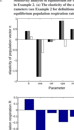
Example 2 (Metabolic population size inTribolium) Flour beetles of the genus Tribol-ium have been the subject of a long series of experiments on nonlinear population dy-namics (reviewed by Cushing et al. 2003). Triboliumlives in stored flour. In addition to feeding on the flour, adults and larvae cannibalize eggs, and adults cannibalize pupae. These interactions are the source of nonlinearity in the demography, and are captured in a three-stage (larvae, pupae, and adults) model. The projection matrix is
A[θ,n] =
1−0µl 00 bexp(−celn01−cean3) 0 exp(−cpan3) 1−µa
(44)
whereb is the clutch size,cea,cel, and cpaare rates of cannibalism (of eggs by adults,
eggs by larvae, and pupae by adults, respectively), and µl andµa are larval and adult
mortalities (the mortality of pupae, in these laboratory conditions, is effectively zero). Parameter values from an experiment reported by Costantino et al. (1997)
b = 6.598
cea = 1.155×10⁻²
cel = 1.209×10⁻²
cpa = 4.7×10⁻³
µa = 7.729×10⁻³
µl = 2.055×10⁻¹
produce a stable equilibrium
ˆ
n=
2218..60 385.2
. (45) ♦
The sensitivity ofnˆis calculated using (23). However, the damage caused byTriboliumas a pest of stored grain products might well depend more on metabolism than on numbers. Emekci et al. (2001) estimated the metabolic rates of larvae, pupae, and adults as 9, 1, and 4.5µl CO2h−1, respectively. We define the metabolic population size asNm(t) =cTn(t)
wherecT=¡ 9 1 4.5 ¢, and calculate the sensitivity and elasticity ofNˆ
musing (42)
Figure 1 shows the elasticity ofnˆ andNˆmto each of the parameters. The elasticities
are diverse and perhaps counterintuitive. Increases in fecundity increase the equilibrium density of all stages; increases in the cannibalism of eggs by adults reduces the density of all stages. But increased cannibalism of pupae by adults increases the density of larvae and pupae, as does an increase in the mortality of adults.
When the stages are weighted by their metabolic rate, the elasticity ofNˆmto fecundity
is positive, but the elasticities to all the other paramters (cannibalism rates and mortalities) are negative. The positive effects ofcpa and µa on nˆ disappear when the stages are
weighted according to metabolism.
4. Environmental feedback models
Environmental (or economic) feedback models write the vital rates as functions of some environmental variable, which in turn depends on population density. Feedback models may be static or dynamic. In static feedback models, the environment depends only on current conditions, with no inherent dynamics of its own. In dynamic feedback models, the environment can have dynamics as complicated as those of the population (e.g., if the environmental variable was the abundance of a prey species, affecting the dynamics of a predator species). The sensitivity analysis of dynamic feedback models is given in Section 8.4.
A static feedback model can be written
n(t+ 1) = A[θ,n(t),g(t)]n(t) (46)
g(t) = g[θ,n(t)] (47)
whereg(t)is a vector (of dimensionq×1) describing the ecological or economic aspects of the environment on which the vital rates depend. As written here, the model admits the possibility that the vital rates inA might depend directly on nas well as on the environment.
At equilibrium
ˆ
n = A[θ,nˆ,gˆ]ˆn (48)
ˆ
g = g[θ,ˆg]. (49)
Differentiating these expressions gives
dnˆ = A(dnˆ) + (dA)ˆn (50)
dgˆ = ∂ˆg ∂θTdθ+
∂ˆg
Figure 1: Sensitivity analysis of equilibrium for the flour beetleTribolium
in Example 2. (a) The elasticity of the equilibriumnˆto the pa-rameters (see Example 2 for definitions). (b) The elasticity of the equilibrium population respiration rateNˆmto the parameters
b cea cel cpa mua mul
−2 −1.5 −1 −0.5 0 0.5 1
Parameter
elasticity of population vector n
Larvae Pupae Adults
(a)
b cea cel cpa mua mul
−0.8 −0.7 −0.6 −0.5 −0.4 −0.3 −0.2 −0.1 0 0.1 0.2
Parameter
elasticity of population respiration R
Applying the vec operator to (50) and expandingdvecAbives
dnˆ = (ˆnT⊗I
s) ·
∂vecA
∂θT dθ+
∂A
∂gTdgˆ ¸
+Adnˆ. (52)
Substituting (51) fordgˆand rearranging gives
dnˆ = (ˆnT⊗I
s) ·
∂vecA
∂θT +
∂vecA
∂gT ∂ˆg
∂θT ¸
dθ
+ ·
A+ (ˆnT⊗I
s)∂vecA ∂gT
∂ˆg
∂nT ¸
dnˆ. (53)
Solving fordnˆand applying the identification theorem yields
dnˆ
dθT =
·
Is−A−(ˆnT⊗Is)∂vecA ∂gT
∂ˆg
∂nT ¸−1
×(ˆn⊗Is) ·
∂vecA
∂θT +
∂vecA
∂gT ∂gˆ ∂θT
¸
. (54)
A,g, and all derivatives are evaluated at(ˆn,gˆ). A comparison of (54) with (23) shows that including the feedback mechanism has simply writtendvecA/dnTanddvecA/dθT in terms ofgusing the chain rule.
The environmental variablegmay be of interest in its own right (e.g., in the food ratio model of Lee and Tuljapurkar (2007), in which it is a measure of well-being, measured in terms of food per individual). The sensitivity ofgˆat equilibrium is
dˆg
dθT = ∂gˆ ∂θT +
∂ˆg
∂n
dnˆ
dθT (55)
wheredˆg/dθT
is given by (51) and (dnˆ/dθT
) by (54).
5. Subsidized populations and competition for space
local fertility (e.g., Almany et al. 2007). Subsidized models have been used to analyze conservation programs in which captive-reared animals are released into a wild or re-established population (Sarrazin and Legendre 2000). They have been applied to the demography of human organizations (e.g., schools, businesses, learned societies; Gani 1963, Pollard 1968, Bartholomew 1982). Wilson (2004) reported that, as of 2004, more than half of humans lived in countries or regions in which fertility was below replacement level. Immigration into such countries is form of subsidy that can be explored with these models.
In the simplest subsidized models, both local demography and recruitment are density-independent. Alternatively, recruitment may depend on some resource (e.g., space) whose availability depends on the local population, or the local demography after settlement is density-dependent. All three cases can lead to equilibrium populations.
5.1 Density-independent subsidized populations
The model,
n(t+ 1) =A[θ]n(t) +b[θ], (56)
includes a subsidy vectorbgiving the input of individuals to the population.5 The
param-etersθmay affectAorb, or both. If the fertility appearing inAis below replacement, so thatλ <1, then a stable equilibriumnˆexists.6This equilibrium satisfies
ˆ
n = Anˆ+b (57)
= (Is−A)−1b. (58)
Differentiating (57) and applying the vec operator yields
dnˆ = (ˆnT⊗I
s)dvecA+A(dnˆ) +db (59)
Solving fordnˆ and applying the chain rule gives the sensitivity of the equilibrium,
dnˆ
dθT = (Is−A)
−1
½ (ˆnT⊗I
s)dvecA
dθT +
db
dθT ¾
. (60)
5The same model could describe harvest ifb≤0(e.g, Hauser et al. 2006). This form of harvest produces
unstable equilibria, and is not considered further here.
6Ifλ >1, the population grows exponentially and the subsidy eventually becomes negligible. The
equi-librium in this case is non-positive (and hence biologically irrelevant) and unstable. Ifλ = 1then the
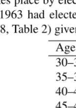
Example 3 (The Australian Academy of Sciences) Most human organizations are sub-sidized; recruits (new students in a school, new employees in a company) come from outside, not from local reproduction. In an early example of a subsidized population model, Pollard (1968) analyzed the age structure of the Australian Academy of Sciences, recruitment to which takes place by election.7 The Academy had been founded in 1954,
and between 1955 and 1963 had elected about 6 new Fellows each year, with an age distribution (Pollard 1968, Table 2) given by
Age Percent
30–34 0.0
35–39 12.2
40–44 24.5
45–49 26.5
50–54 20.4
55–59 4.1
60–64 10.2
65–69 2.0
♦
Pollard interpolated this distribution to 1-year age classes, and combined it with a 1954 life table for Australian males8to construct a model of the form (56) and calculated the
equilibrium size and age composition of the Academy. Here, I have used the male life table for Australia 1953–1955 in Keyfitz and Flieger (1968, p. 558) to construct an age-classified matrixAwith age-specific probabilities of survivalPi on its subdiagonal and
zeros elsewhere. Were these vital rates and the age distribution of the subsidy vector to remain constant, the Academy would reach an equilibrium size ofNˆ = 149.5with an age distributionnˆshown in Figure 2a.
As parameters, consider the age-specific mortality ratesµi=−logPi, and define the
parameter vectorθ=¡ µ1 µ2 . . .
¢T
. Equation (60) then gives the sensitivity of the equilibrium population to changes in age-specific mortality. The sensitivity of the total size of the Academy,Nˆ = eTnˆ, calculated using (38), is shown in Figure 2b. It shows that increases in mortality reduceNˆ(not surprising), with the greatest effect coming from changes in mortality at ages 48–58.
Because learned societies are often concerned with their age distributions, Pollard (1968) examined the proportion of members over age 70. At equilibrium, this proportion isRˆ = 0.26. The sensitivity dR/dˆ θT, calculated using (40), is shown in Figure 2c.
7Pollard’s paper is remarkable for its treatment of both deterministic and stochastic models, but here I
consider only the deterministic case.
8Only one woman, the redoubtable geologist Dorothy Hill in 1956, was elected to the Academy prior to
Figure 2: Analysis of the equilibrium of a linear subsidized model for the Australian Academy of Science, based on Pollard (1968). (a) The equilibrium age structure of the Academy, assuming recruitment of 6 members per year. (b) The sensitivity, to changes in age-specific mortality, of the number of members. (c) The sensitivity, to changes in age-specific mortality, of the proportion of members over 70 years old
20 30 40 50 60 70 80 90
0 0.5 1 1.5 2 2.5 3 3.5 4 4.5 5
Age
Equilibrium number
(a)
20 30 40 50 60 70 80 90
−90 −80 −70 −60 −50 −40 −30 −20 −10 0
Age
Sensitivity of N to mortality
(b)
20 30 40 50 60 70 80 90
−0.2 −0.15 −0.1 −0.05 0 0.05
Age
Sensitivity of proportion >70 to mortality
(c)
Increases in mortality before age 48 would increase the proportion of members over 70, while increases in mortality after age 48 would decrease it.9
9It is possible to calculate the average age of the Academy, and its sensitivity, using results to be introduced
5.2 Linear subsidized models with competition for space
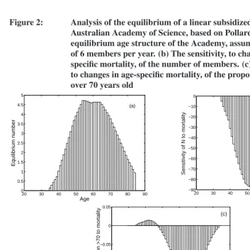
Recruitment in subsidized populations may be limited by the availability of a resource. Roughgarden et al. (1985; see also Pascual and Caswell 1991) presented a model for a population of sessile organisms, such as barnacles, in which recruitment is limited by available space. Barnacles10produce larvae that disperse in the plankton for several weeks
before settling onto a rock surface or other suitable substrate, after which they no longer move.
Roughgarden’s model supposes that settlement is proportional to the free spaceF(t). Thus the subsidy vector is
b(t) =¡ φF(t) 0 · · · 0 ¢T
, (61)
whereφis the settlement rate per unit of free space, and is determined by the pool of available larvae. The free space is the difference between the total areaAand the space occupied by the population,
F(t) =A−gTn(t) (62)
wheregis a vector of stage-specific basal areas. Suppose that all locally-produced larvae are advected away, so that the first row ofAis zero. Then, substituting (62) into (61) and rearranging gives
n(t+ 1) =Bn(t) +¡ φA 0 · · · 0 ¢T (63)
where
B=
−φg1 −φg2 · · · −φgs a21 a22 · · · a2s
..
. ... . .. ...
as1 as2 · · · ass
. (64)
Although it includes competition for space, the model is linear. The equilibriumnˆ of (63) is stable if the spectral radius ofBis less than one.11 The formula (60) gives the
sensitivity of this equilibrium to changes in the vital rates, the settlement rate, or the individual growth rate. This model might apply to any situation where the recruitment of new individuals depends on the availability of a resource (space, jobs, housing) that can be monopolized by residents.
Example 4 (Intertidal barnacles) Gaines and Roughgarden (1985) modelled a popula-tion of the barnacleBalanus glandulain central California. In one site (denoted KLM
10The temptation to draw analogies between barnacles and the members of learned academies is almost
irresistible.
11BecauseBcontains negative elements, its dominant eigenvalue may be complex or negative, leading to
in their paper), they reported age-independent survival with a probability ofPi = 0.985
per week, i = 1, . . . ,52. The growth in basal area of an individual barnacle could be described by gx = π(ρx)2, where xis age in weeks and ρis the radial growth rate
(ρ= 0.0041cm/wk). The mean settlement rate wasφ= 0.107. The matrixBcontains survival probabilitiesPion the subdiagonal, terms of the form−φgiin the first row, and
zeros elsewhere.
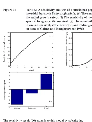
The equilibrium populationnˆ has an exponential age distribution (Figure 3a). It is scaled here relative to total area, soA= 1. The equilibrium proportion of free space is
ˆ
F = 0.865.
To calculate sensitivities, letθ=¡ P1 · · · P52
¢
. Some of the possible sensitiv-ities are shown in Figure 3. Increasing survival at agej(agesj = 10,20,40are shown) reduces the abundance of ages younger thanjand increases the abundance of ages older thanj(Figure 3b). A perturbation to a parameter, call itξ, that affects survival at all ages has the effect
dnˆ
dξ =
dnˆ dθT
dθ
dξ =
dnˆ
dθe (65)
whereeis a vector of ones. An increase in overall survival would reduce the abundance of age classes 1–6 and increase the abundance of older age classes (Figure 3c).
The sensitivity of nˆ to the larval settlement rateφis obtained from (60) by setting
dvecB/dφ=0s2×1, and
db
dφ =
¡ ˆ
F 0 · · · 0 ¢T
Not surprisingly, increases inφincreasenˆ, with the largest effect on the young age classes (Figure 3d). The sensitivity ofnˆto the radial growth rateρis obtained by writing
dvecB
dρ =
dvecB
dgT dg
dρ (66)
This sensitivity is negative, with the greatest impact on young age classes (Figure 3e). Finally, the sensitivity of the equilibrium free space is given by
dFˆ dθT =
dFˆ dnT
dnˆ dθT =−g
Tdnˆ
dθT (67) ♦
Figure 3: A sensitivity analysis of a subsidized population of the intertidal barnacleBalanus glandula. (a) The equilibrium populationnˆ
(scaled relative to a unit of areaA = 1). (b) The sensitivity ofnˆ
to a change in survival at agesj = 10,20,40. (c) The sensitivity of
ˆ
nto changes in overall survival at all ages. (d) The sensitivity ofnˆ
to the settlement rateφper unit area.Continued on next figure.
0 10 20 30 40 50 60
0.04 0.05 0.06 0.07 0.08 0.09 0.1
Age
Equilibrium population
(a)
0 10 20 30 40 50 60
−0.02 −0.01 0 0.01 0.02 0.03 0.04 0.05 0.06 0.07 0.08
Sensitivity of
n
to survival at age j
Age i
(b)
j=10 20 40
0 10 20 30 40 50 60
−0.5 0 0.5 1 1.5 2 2.5
Sensitivity of
n
to overall survival
Age i
(c)
0 10 20 30 40 50 60
0.35 0.4 0.45 0.5 0.55 0.6 0.65 0.7 0.75
Sensitivity olf
n
to settlement
φ
Age i
(d)
5.3 Density-dependent subsidized models
Once individuals to the population, they may experience a variety of density-dependent effects. For example, Gaines and Roughgarden (1985) found that increased barnacle den-sity led to increased mortality due to attack by the starfishPisaster ochraceus. A model incorporating such effects would be written
Figure 3: (cont’d.) A sensitivity analysis of a subsidized population of the intertidal barnacleBalanus glandula. (e) The sensitivity ofnˆ to the radial growth rateρ. (f) The sensitivity of the equilibrium free spaceFˆ to age-specific survival. (g) The sensitivity ofFˆto changes in overall survival, settlement rate, and radial growth rate. Based on data of Gaines and Roughgarden (1985)
0 10 20 30 40 50 60
−3.2 −3 −2.8 −2.6 −2.4 −2.2 −2 −1.8 −1.6 −1.4
Sensitivity of
n
to growth rate
ρ
Age i
(e)
0 10 20 30 40 50 60
−0.12 −0.1 −0.08 −0.06 −0.04 −0.02 0
Sensitivity of free space
F
to survival
p(j)
Age j
(f)
Survival Settlement Growth
−5 −4 −3 −2 −1 0 1 2 3 4 5
Sensitivity of free space
(g)
The sensitivity result (60) extends to this model by substituting
dvecA= ∂vecA
∂θT dθ+
∂vecA
∂nT dnˆ (69)
into (59) and solving fordnˆ, to obtain
dnˆ dθT =
µ
Is−A−(ˆnT⊗Is)∂vecA ∂nT
¶−1½
(ˆnT⊗I
s)∂vecA
∂θT +
db
dθT ¾
. (70)
6. Sensitivity of proportional age and stage distributions
The linear modeln(t+ 1) = An(t) will, ifA is primitive, converge to a stable age or stage distribution. But while the dynamics of the population vectorn(t)are linear, but the dynamics of theproportionalpopulation structure are nonlinear (e.g., Tuljapurkar 1997). We can take advantage of this to analyze the sensitivity of proportional structures by writing them as equilibria of nonlinear maps.
Letpdenote the proportional stage structure vector (p≥0,eTp= 1). The dynamics ofp(t)satisfy
p(t+ 1) = Ap(t)
kAp(t)k. (71)
The stable stage distribution is an equilibrium of (71).
6.1 The stable stage distribution and reproductive value
The sensitivity of the stable stage distribution has been approached as an eigenvector per-turbation problem (e.g., Caswell 1982, 2001, Section 9.4, Kirkland and Neumann 1994), but those calculations are complicated. Analysis of the equilibrium of the nonlinear model (71) is much easier.
The stable stage distribution satisfies
ˆ
p= Apˆ
eTApˆ (72)
where the 1-norm can be replaced byeTApˆ becausepˆ is non-negative. Differentiating both sides gives
dpˆ = 1
(eTApˆ)2 ·
eTApˆ(dA)ˆp+eTApAˆ (dpˆ)−Apeˆ T(dA)ˆp−Apeˆ TA(dpˆ) ¸
(73)
Note thatApˆ =λpˆ andeTApˆ =λ, whereλis the dominant eigenvalue ofA. Making these substitutions and applying the vec operator to both sides gives
λ dpˆ =£(ˆpT⊗I
s)−(ˆpT⊗peˆ T) ¤
dvecA+ [A−peˆ TA]dpˆ (74)
Solving fordpˆand applying the chain rule gives
dpˆ
dθT = (λIs−A+ ˆpe
TA)−1(ˆpT⊗I
s−pˆT⊗peˆ T)
dvecA
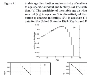
Figure 4: Stable age distribution and sensitivity of stable age distribution to age-specific survival and fertility. (a) The stable age distribu-tion. (b) The sensitivity of the stable age distribution to changes in survival (P5) in age class 5. (c) Sensitivity of the stable age
distri-bution to changes in fertility (F5) in age class 5. Based on life table
data for the United States in 1985 (Keyfitz and Flieger 1990)
0 20 40 60 80 100
0.03 0.035 0.04 0.045 0.05 0.055 0.06 0.065
Age
Stable age distribution
(a)
0 5 10 15 20
−0.03 −0.02 −0.01 0 0.01 0.02 0.03 0.04
Age class i
Sensitivity of
p
to P
5
(b)
0 5 10 15 20
−0.08 −0.06 −0.04 −0.02 0 0.02 0.04 0.06 0.08 0.1
Age class i
Sensitivity of
p
to F
5
(c)
Example 5 (A human age distribution) As an example, consider the age distribution of the population of the United States in 1985 (data from Keyfitz and Flieger 1990). These vital rates yield a declining population (λ = 0.975) and an age distribution skewed to-wards older ages (Figure 4). Applying (75) yields the sensitivity of pˆ to age-specific survival probabilitiesPi and fertilitiesFi, where age classesi = 1, . . . ,18correspond
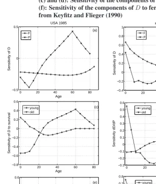
Figure 5: Sensitivity of the dependency ratioD, and of its old and young components, to age-specific survival and fertility. Left: calcu-lated from the stable age distribution of the United States in 1985. Right: calculated from the stable age distribution of Kuwait in 1970. (a) and (b): Sensitivity ofDto survival (Pi) and fertility (Fi). (c) and (d): Sensitivity of the components ofDto survival. (e) and (f): Sensitivity of the components ofDto fertility. Life table data from Keyfitz and Flieger (1990)
0 20 40 60 80
−0.5 0 0.5
Age
Sensitivity of D
USA 1985
(a)
F P
0 20 40 60 80
−0.4 −0.2 0 0.2 0.4 0.6 0.8 1 Age
Sensitivity of D
Kuwait 1970
(b)
F P
0 20 40 60 80
−0.8 −0.6 −0.4 −0.2 0 0.2 0.4 0.6 Age Sensitivity of D to survival (c) young old
0 20 40 60 80
−0.3 −0.2 −0.1 0 0.1 0.2 0.3 0.4 0.5 0.6 Age Sensitivity dD/dP (d) young old
0 20 40 60 80
−0.8 −0.6 −0.4 −0.2 0 0.2 0.4 0.6 Age Sensitivity of D to fertility (e) young old
0 20 40 60 80
classes, at the expense of younger and older age classes. Increasing fertility at a given age increases the abundance of young age classes at the expense of older age classes.
A similar approach gives the sensitivity of the reproductive value vectorv, given by the left eigenvector ofAcorresponding toλ. Reproductive value is customarily scaled so thatv1= 1. Scaled in this way,vsatisfies
ˆ
vT= vˆ TA
ˆ
vTAe1 (76)
wheree1 is a vector with 1 in the first entry and zeros elsewhere. Differentiating both sides gives
dvˆT= 1
(ˆvTAe1)2 £
ˆ
vTAe1(dvˆT)A+ ˆvTAe1vˆT(dA)−(dvˆT)Ae1vˆTA−vˆT(dA)e1vˆTA¤
(77) ButvˆTA = λvˆT andvˆTAe1 = λ. Making these substitutions and applying the vec operator (remembering that vecvT=v) gives
λdv=£(Is⊗ˆvT)−(ˆveT1⊗vˆT)
¤
dvecA+ (AT−veˆ T
1AT)dv. (78)
Solving fordvand using the chain rule gives
dvˆ
dθT = (λIs−A T+ ˆveT
1AT)
−1£
(Is⊗vˆT)−(ˆveT1⊗vˆT)
¤dvecA
dθT (79)
6.2 Sensitivity of the dependency ratio
The dependency ratio characterizes an age distribution by the relative abundance of two groups, one assumed to be dependent and the other productive (e.g., Keyfitz and Flieger 1990, p. 32; Li and Tuljapurkar, unpublished). It is often assumed that persons younger than 15 or older than 65 are dependent on productive individuals between 15 and 65. The dependency ratio is defined as
D= a
Tpˆ
bTpˆ (80)
whereais a vector with ones for the dependent ages and zeros otherwise, andbis its complement. Applying equation (40) for the sensitivity of a ratio gives
dD dθT =
Ã
bTpaˆ T−aTpbˆ T (bTpˆ)2
! dpˆ
dθT. (81)
This result can be generalized in several ways. The analysis may be performed sepa-rately for the dependent young and the dependent old, by suitable modification ofaand
b. These two components are likely to be influenced by different demographic factors and can respond to perturbations in opposite directions. The0−1vectorsaandbmay be replaced by vectors of weights; e.g., age-specific consumption and age-specific income (Li and Tuljapurkar, unpublished). The analysis applies to stage-classified models, pro-vided that dependent and independent stages can be identified. It also applies to nonlinear models, with the stable stage distributionpˆ replaced by the equilibrium populationnˆin (81). It can be extended to transient dynamics, where the age distribution, and thus the dependency ratio, varies over time (Caswell 2007a). Finally, the sensitivity (81) makes it possible to carry out LTRE analyses (Caswell 2001, Chapter 10) to decompose differences in dependency ratios into components due to differences in each of the vital rates.
Example 5 ((cont’d) Dependency ratios in human populations.) The United States in 1985 had a set of vital rates leading to a low growth rate (λ= 0.975), and a relatively low dependency ratio, dominated by the old. Kuwait in 1970, in contrast, had a high growth rate (λ = 1.210) and one of the highest dependency ratios listed in the compilation of Keyfitz and Flieger (1990), dominated by the young:
U.S.A. 1985 Kuwait 1970
D 0.668 1.025
Dy 0.260 0.956
Do 0.406 0.069 ♦
whereDy andDoare the dependency ratios calculated for the young and old separately.
The sensitivities ofD,Dy, andDoto changes in age-specific survival and fertility are
shown in Figure 5. The responses ofD to changes in the vital rates differ between the two countries. In the U.S., increases in fertility would reduceD. In Kuwait, increases in fertility (especially at young ages) would increaseD. In the U.S., increases in sur-vival12before age 30 reduceD; increases after age 30 increaseD. In Kuwait, increases
in survival, except at very young and very old ages, reduceD.
BreakingDinto its young and old components helps to explain these differences. In both countries, there is a crossover in survival effects. Increases in survival at early ages increaseDy and reduceDo. At later ages, increases in survival reduceDyand increase Do. Increases in fertility increaseDy and reduceDo. In the U.S. population, both these
effects are large, with the negative effect onDolarger than the positive effect onDy. In
the Kuwaiti population, the positive effect onDyis much greater than the negative effect
onDo.
12Or, equivalently, reductions in mortality. For these parameter values, the sensitivity to mortality is
6.3 Sensitivity of mean age and related quantities
From an age distributionpˆ, it is possible to compute the mean age of any age-specific property (e.g., production of children, collection of retirement benefits, exposure to toxic chemicals; see Chu 1998, p. 26 for general discussions). The most familiar of these is the mean age of reproduction, which is one measure of generation time (Coale 1972).
Letfbe a vector of age-specific per-capita fertilities. The age distribution of offspring production is thenf ◦pˆ, where◦is the Hadamard, or element-by-element product. The mean age of the mothers of these offspring is obtained by normalizingf ◦pˆto sum to 1 and taking the mean over the resulting distribution,
¯ af = c
T(f◦pˆ)
eT(f ◦pˆ) (82)
where
cT=¡ 1 2 · · · s ¢,
withsas the last age class.
Now differentiate¯af, following the now-familiar rules for ratios. The differential of the Hadamard product of two vectors isd(a◦b) =diag(a)db+diag(b)da. The result is
d¯af
dθT = Ã
eT(f◦pˆ)cT−cT(f◦pˆ)eT (fTpˆ)2
! µ
diag(f)dpˆ
dθT +diag(ˆp) df
dθT 
(83)
wheredpˆ/dθT
is given by (75).
This result can be generalized in several ways. Settingf =emakes the age-specific property that of simply being alive, anda¯e = cTeis then the mean age of the stable population, the sensitivity of which is
d¯a dθT =c
Tdpˆ
dθT (84)
The calculations can also be applied to the equilibrium population in a nonlinear model by substitutingnˆforpˆ. They apply directly to stage-classified models with stages defined on an interval scale (e.g., size classes), in which case they give, e.g., the mean size at reproduction. If the stages are not evenly spaced, thencwould be replaced by
cT=¡ x
1 x2 · · · xs ¢
(85)
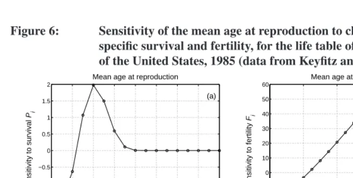
Figure 6: Sensitivity of the mean age at reproduction to changes in age-specific survival and fertility, for the life table of the population of the United States, 1985 (data from Keyfitz and Flieger 1990)
0 10 20 30 40 50 60 70 80
−2 −1.5 −1 −0.5 0 0.5 1 1.5 2
Age i
Sensitivity to survival
Pi
Mean age at reproduction
(a)
0 20 40 60 80 100
−30 −20 −10 0 10 20 30 40 50 60
Age i
Sensitivity to fertility
Fi
Mean age at reproduction
(b)
♦
Example 5 ((cont’d.) Mean age of reproduction.) The mean age of reproduction in the stable age distribution of the United States in 1985 was¯af = 24.02years (using the mid-points of the 5-year age intervals as the measure of age). The sensitivities of¯afto changes in age-specific survival and fertility are shown in Figure 6. Increases in survival prior to age 15 reduce¯af. Increases in survival after age 45 have almost no effect on¯af, because fertility is essentially zero after this age. Between age 15 and age 45, increases in survival increase the mean age of reproduction.
Increases in fertility reduce¯af if they happen before age 25 and increase¯af if they happen after age 25. These sensitivities are quite large, although this is somewhat irrele-vant since the largest sensitivities are for ages at which fertility is zero and unlikely to be modified.
6.4 Sensitivity of variance in age
We can also calculate the sensitivity of the higher moments. For example, the variance in the age at reproduction is
Vf =a2f −(¯af)2. (86)
This variance might, for example, be useful as a measure of the extent of iteroparity. The sensitivity ofVf to changes in parameters is obtained by writing the first term as
a2 f =
(c◦c)T(f◦pˆ)
and then differentiating
dVf =d
³ a2
f
´
−2¯af (d¯af). (88)
The final result is
dVf
dθT =
Ã
eT(f◦pˆ)(c◦c)T−(c◦c)T(f ◦pˆ)eT (fTpˆ)2
!
×
µ
diag(f)dpˆ
dθT +diag(ˆp) df
dθT 
−2¯afd¯af
dθT. (89)
wheredpˆ/dθTis given by (75) andd¯a
f/dθTis given by (83).
7. Frequency-dependent two-sex models
In sexually reproducing species, nonlinearity can arise from the dependence of reproduc-tion on the relative abundance of males and females. This dependence is captured in a marriage function or mating rule (e.g., McFarland 1972, Pollak 1987, 1990). When the vital rates depend only on the relative, rather than the absolute, abundance of males and females, thenA[θ,n]is homogeneous of degree 0 inn; i.e.,
A[θ, cn] =A[θ,n] for anyc6= 0. (90)
Such models are called frequency-dependent (Caswell and Weeks 1986, Caswell 2001) to distinguish them from density-dependent nonlinear models that do not have this homo-geneity property.
Because of the homogeneity ofA[θ,n], frequency-dependent models do not converge to an equilibrium densitynˆ. Instead, there may exist13 a stable equilibrium proportional
structurepˆto which the population will converge, at which point it grows exponentially at a rateλgiven by the dominant eigenvalue ofA[θ,pˆ]. Thus sensitivity analysis of two-sex models must include both the population structure and the population growth rate.
7.1 Sensitivity of the population structure
The equilibrium proportional population structurepˆsatisfies
ˆ
p= A[θ,pˆ] ˆp
kA[θ,pˆ] ˆpk (91)
13A sufficient, but not necessary, condition for the existence of an equilibrium is thatAcannot map a nonzero
wherepˆi≥0andeTpˆ = 1. Differentiating (91) gives
dpˆ =e
TApˆ£(dA)ˆp+A(dpˆ)¤−Apˆ£eT(dA)ˆp+eTA(dpˆ)¤
(eTApˆ)2 . (92)
Making the substitutionsApˆ =λpˆ andeTApˆ =λand rearranging gives
λdpˆ= (dA)ˆp+A(dpˆ)−peˆ T(dA)ˆp−peˆ TA(dpˆ). (93)
Applying the vec operator to both sides, expandingdvecA, invoking the chain rule, and solving fordpˆ/dθTgives
dpˆ dθT =
·
λIs−A+ ˆpeTA− £
ˆ
pT⊗(I
s−peˆ T)
¤∂vecA
∂pT ¸−1·
ˆ
pT⊗(I
s−peˆ T) ¸
∂vecA
∂θT (94) whereAand all derivatives are evaluated atpˆ. Note that (94) differs from the expres-sion (75) for the stable stage distribution in the linear model only in the term involving
∂vecA/∂pT, which of course is zero in the linear model.
7.2 Sensitivity of population growth rate
Because a population with the equilibrium structure grows exponentially, I once suggested treatingA[θ,pˆ]as a constant matrix and applying eigenvalue sensitivity analysis to it, in order to examine life history evolution in 2-sex models (Caswell 2001, p. 577). This was incorrect, because it ignored the effect of parameter changes onAthrough their effects on the equilibriumpˆ. A correct calculation obtains the sensitivity ofλincluding effects of parameters on bothAandpˆ.
Note thatpˆ is a right eigenvector ofA[θ,pˆ]corresponding toλ. Letvbe the corre-sponding left eigenvector, wherevTA[θ,pˆ] =λvTandvTpˆ= 1. Then
dλ=vT(dA)ˆp (95)
(Caswell 1978). Apply the vec operator and Roth’s theorem to get
dλ= (ˆpT⊗vT)dvecA. (96)
ExpandingdvecAgives
dλ dθT = (ˆp
T⊗vT) ·
∂vecA
∂θT +
∂vecA
∂pˆT dpˆ dθT ¸
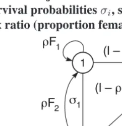
Figure 7: Life cycle graph for the 2-sex model for passerine birds (Legendre et al. 1999). Stages 1 and 2 are juvenile and adult females; stages 3 and 4 are juvenile and adult males. Parameters are stage specific survival probabilitiesσi, stage-specific fertilitiesFi, and primary sex ratio (proportion female)ρ
1
2
3
4
ρF1
(l – ρ)F1
(l – ρ)F2
ρF2
σ2 σ4
σ3
σ1
whereA,v, and the derivatives ofAare all evaluated at the equilibriumpˆ, anddpˆ/dθT is given by (94).
Note that λis the invasion exponent for this model, and thus the sensitivity ofλto a parameter gives the selection gradient on that parameter. Tuljapurkar et al. (2007) used this fact to explore the effect of male fertility patterns on the evolution of aging; the sensitivity (97) could be used to generalize such results.
Although two-sex models are an important case of homogeneous models, they are not the only case. Keyfitz’s (1972a) interpretation of the Easterlin hypothesis describes fer-tility as dependent on only the relative, not absolute, size of a cohort. A model based on this premise would be frequency-dependent (homogeneous) and would lead to an expo-nentially growing population to which (97) would be applicable.
Example 6 (A two-sex model for passerine birds) Legendre et al. (1999) used a frequency-dependent two-sex model to study the introductions of passerine birds to New Zealand. The life cycle includes two age classes (first year and older) for females and for males. The life cycle graph is shown in Figure 7. The numbers of females and males are
Nf =n1+n2andNm=n3+n4, respectively.
Because passerines are typically monogamous within a breeding season, and assum-ing that matassum-ing is indiscriminate with respect to age, Legendre et al. (1999) used as a mating function