Consideration of Body Forces within Finite Element Analysis

*Corr. Author’s Address: University of Bayreuth, Faculty of Engineering Science, Department of Engineering Design and CAD, 303

0 INTRODUCTION

The swift development in recent decades towards more powerful computers has allowed the widespread use of complex simulation programs based on numerical methods. Thus, finite element analysis (FEA) is now an established standard procedure in many areas of numerical strength analysis. Despite the increasing computing power, the endeavour is to develop more efficient algorithms and thus to minimize the computation time during the FEA.

The main idea of the FEA is to partition a continuum into a finite number of finitely large sub-continua [1] to [3]. Such discretized elements are referred to as finite elements (FE). Their nodes act as joints between neighbouring elements and as target points for the specification of loads and displacement boundary conditions. The solid deforms under mechanical load, resulting in a deformation of each finite element. The displacement of any point x within an element is specified by the vector field u. The location and displacement of any point inside a finite element are interpolated from the position Pi

and the displacement di of the element nodes.

These nodal displacements are computed via a discretized formulation of the mechanical momentum equation. Starting from the geometrical discretization of the continuum, one possible approach for the derivation of the discretized momentum equation is the Galerkin method [1], [2] and [4]. In the case of a static equilibrium problem, this ultimately leads to a

system of linear equations for determining the nodal displacements:

K⋅ =d R R s+ b. (1)

Matrix K is the stiffness matrix and the vectors



RS and 

Rb represent the load vectors of surface

forces and body forces.

Body forces, such as the weight force, affect almost all technical components and cannot be neglected in stress analysis, e.g. in areas such as structural engineering. They affect the whole element from a physical point of view, but they are proportionately distributed to the element nodes within the finite element method. For each element, the equivalent nodal forces can be calculated as follows [5]:

 _

Rbe gdV

Ve

=

_∫∫∫

_NTρ

, (2)

where N is the matrix of the shape functions and ρg describes the mass density and the gravitational constant. If the mass density and the gravitational factor are assumed to be constant for each finite element, both quantities can be put outside the integral, leading to the following expression:

 _

R_be dV g

Ve

=

∫∫∫

NT ⋅ρ

. (3)

The vector Rb in Eq. (1) can be calculated by

assembling each elemental force vector into one global force vector [2]:

Consideration of Body Forces within Finite Element Analysis

Glenk, C. – Hüter, F. – Billenstein, D. – Rieg, F.

Christian Glenk* _{– Florian Hüter – Daniel Billenstein – Frank Rieg}

University of Bayreuth, Faculty of Engineering Science, Germany

The finite element analysis (FEA) is an established numerical method for the mechanical analysis of structural components, which cannot be analytically described sufficiently well. Despite ever-increasing computing power, the efficiency enhancement of the calculation methods and their computational implementation is one of the highest development goals in this field. This article shows an efficient method for the calculation of weight forces that is based on a factorization of the volume integral so that the integration is independent of the global node coordinates of the finite element mesh and solely dependent on the shape functions of the element type. The numerical integration can thus be done in advance, and the resultant numerical values can be tabulated in the finite element software. No quadrature needs to be performed during the program runtime. This approach leads to a reduction of the computing effort and time.

Keywords: finite element analysis, body force, weight force, numerical integration, Gaussian quadrature

Highlights

• Efficient method for the calculation of body forces within finite element analysis was implemented. • Factorization of the volume integral makes the integration independent of the global node coordinates.

• Most of the computational effort, i.e. numerical integration, does not need to be performed during the FE-program runtime. • Computing effort and computation time can be reduced.

 

Rb Rbe

e

=

∑

. (4)

In this paper, we present a mathematical approach to a time-efficient calculation of the volume integral in Eq. (3).

1 ELEMENT DESCRIPTION AND NUMERICAL INTEGRATION

Interpolation polynomials are used to describe the displacement field u within a finite element, which are composed of the shape functions Ni and the

displacement vectors di of each element node.

Typically, the following formula is used in the FEM literature [1], [5] and [6]:

 

u r s t N r s t di i

i

( , , )≈

∑

( , , )⋅ . (5)

The location dependency of the displacement field is included in the shape functions. If these functions were dependent on the global Cartesian coordinates (x, y, z), the shape functions Ni would have

to be determined individually for each finite element of the structure. To avoid this effort, a coordinate transformation into a generally curvilinear element coordinate system (r, s, t) is typically performed within the finite element method. In that way, the finite elements are transformed into their undistorted geometry, which is why this coordinate system is also called the natural coordinate system.

An interpolation approach similar to Eq. (5) is typically used to establish a relation between the global coordinates (x, y, z) and the curvilinear, natural coordinates (r, s, t):

x r s t N r s t Pi _i

i

( , , )≈

∑

( , , ) , (6)

where Ni denotes the shape functions for the

interpolation of the geometry and Pi the node

coordinates in the global Cartesian coordinate system. Generally, the supporting points for the interpolation polynomials of u and do not have to be coincidental [6]. Other or fewer nodes can be used for the calculation of x. If the supporting points are chosen to be identical, the shape functions Ni and N_i

coincide. In this case, the element formulation is called isoparametric [2].

According to Eq. (3), a volume integral must be solved for the calculation of the gravitational nodal forces. If the element formulation is assumed to be isoparametric, the integration can be performed in the natural coordinate system [3]:

 _

R_be drdsdt g

r s t

=

∫∫∫

NT J ⋅

det

( , , )

.

ρ (7)

The term det J denotes the determinant of the Jacobian matrix, also called functional determinant, and is defined as:

detJ= .

∂ ∂ ∂ ∂ ∂ ∂ ∂ ∂ ∂ ∂ ∂ ∂ ∂ ∂ ∂ ∂ ∂ ∂ x r x s x t y r y s y t z r z s z t (8)

The evaluation of the volume integral, shown in Eq. (7), is usually carried out by numerical integration

[3]. Typically, Gaussian quadrature is used in this context [1], which is based on the idea of evaluating the integrand at certain grid points, so-called Gauss points, and calculating the weighted sum [3]:

 _

Rbe a b c T r s ta b c g

c m b m a m ≈

{

}

⋅ = = =

∑

∑

∑

α α α N detJ ( , , ) ρ .

1 1 1

(9)

The parameters (αa, αb, αc) denote the Gaussian

weights, and (ra, sb, tc) are the natural coordinates

of the Gauss points [3]. These parameters might be different for various element geometries. For example, there are Gaussian weights and Gauss points specially developed for triangles and tetrahedrons [1], [7] and

[8].

If the polynomial degree is denoted as p, at least m = (p+1) / 2 supporting points are required to obtain an exact integration [9].

2 FACTORIZATION OF THE JACOBIAN DETERMINANT

During the calculation of the Jacobian determinant, the partial derivatives of the Cartesian coordinates (x, y, z) with respect to the natural coordinates (r, s, t) must be evaluated. If an isoparametric element formulation is assumed, the following equation holds [3]:

detJ=

∂ ∂ ∂ ∂ ∂ ∂ ∂ ∂ ∂ ∂ = = = =

∑

∑

∑

∑

N r x N s x N t x N r y N s i i i n i i i n i i i n j j j n j

1 1 1

1 yy N t y N r z N s z N t z j j n j j j n k k k n k k k n k k k n = = = = =

∑

∑

∑

∑

∑

∂ ∂ ∂ ∂ ∂ ∂ ∂ ∂ 1 1

1 1 1

. (10)

detJ= ∂ ∂ ∂ ∂ ∂ ∂ + ∂ ∂ ∂ ∂ ∂ ∂ = = =

∑

∑

∑

N_r N_s N_t x y z

N r N s N t x

i j k

i j k k n j n i n

k i j

1 1 1

ii j k k n j n i n

j k i

i j k k n j n i n y z N r N s N t x y z = = = = = =

∑

∑

∑

∑

∑

∑

+ ∂ ∂ ∂ ∂ ∂ ∂ 1 1 1 1 1 1 −− ∂ ∂ ∂ ∂ ∂ ∂ − ∂ ∂ ∂ ∂ ∂ ∂ = = =

∑

∑

∑

N_r N_s N_t x y z

N r

N s

N t x y

k j i

i j k k n j n i n

i k j

i j 1 1 1 zz N r N s N t x y z

k k n j n i n

j i k

i j k k n j n i n = = = = = =

∑

∑

∑

∑

∑

∑

− ∂ ∂ ∂ ∂ ∂ ∂ 1 1 1 1 1 1 (11)

By bracketing out the node coordinates, this equation can be rewritten as:

detJ=

∂ ∂ ∂ ∂ ∂ ∂ ∂ ∂ ∂ ∂ ∂ ∂ ∂ ∂ ∂ ∂ ∂ ∂ = =

∑

N r N s N t N r N s N t N r N s N t

i i i

j j j

k k k

k n

j 1 1

nn

i n

i j k

x y z

∑

∑

=

⋅

1

. (12)

According to this equation, the Jacobian determinant can be “factorized” in such a way that the node coordinates (xi, yj, zk) and the partial derivatives

of the shape functions are separated:

detJ= ( , , )⋅ .

= =

=

∑

∑

∑

H r s t Xijk ijk

k n j n i n 1 1 1 (13)

Based on the general properties of determinants

[10], it can be shown that the determinant of the partial differential derivatives Hijk possess the following

properties:

1) Hijk = 0 for i = j and/or j = k and/or k = i,

2) Hijk = –Hjik = Hjki = –Hkji = Hkij = –Hikj.

These properties result from the fact that the rows of Hijk are identical and that interchanging rows leads

to a change of the sign of the determinant.

According to these properties, the following statements can be concluded:

1. To determine the value of all Hijk, it suffices to

calculate solely those Iijk with: i = 1, ..., n – 2, j = i + 1, ..., n – 1, k = j + 1, ..., n.

2. The sign of all Hijk can be determined via property

2).

3. The number of the determinants Hijk to be

calculated decreases from n3 _to n

n

! ( −3)!3!.

To proof these statements, Hijkis considered as

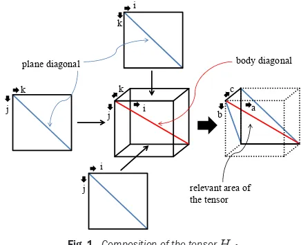
a tensor of third order with n elements per row, i.e. it describes a cube of “edge length” n. According to property 1), all components of this tensor with i = j and/or j = k and/or k = i are equal to zero. All these zero-values Hiik, Hijj and Hkjk are arranged in such a

manner that they form three planes within the cube, which intersect along the body diagonal of the cube, where i = j = k holds. The cube is thereby divided into six tetrahedrons, Fig. 1. These tetrahedrons can be described by the intervals of indices a = 1, ..., n – 2, b = a + 1, ..., n – 1 and c = b + 1, ..., n, where the parameters (a, b, c) are placeholders for each of the six possible permutations of (i, j, k). One possible tetrahedron is defined as i = 1, ..., n – 2, j = i + 1, ..., n – 1, and k = j + 1, ..., n, which is shown in Fig. 1.

i k j k k i j j i

plane diagonal body diagonal

relevant area of the tensor

c

b a

Fig. 1. Composition of the tensorHijk

According to property 2) all other five tetrahedrons have the same entries regarding their absolute value. They only differ in sign. Therefore, it suffices to calculate only one of these six tetrahedrons. All the others can be derived from the first tetrahedron based on property 2), which is why the second statement is valid.

The third statement is verified with an example. If n = 3, i.e. i, j, k = 1, ..., 3, then there are n3 _{= 27}

different “combinations” for the index triple: (i, j, k) = (1, 1, 1), (1, 1, 2), (1, 2, 1), (2, 1, 1) etc. According to property 1), all combinations comprised of at least two identical indices, such as (1, 1, 2) or (3, 3, 3), are of no interest. Consequently, the number of relevant combinations decreases to n! = 6. Furthermore, the sequence of the indices within each index triple is irrelevant according to property 2), i.e. | Hijk | = | Hjik | = | Hkij |, etc. The number of relevant

n n

!

( −3)!3! = 1. For this reason, (1, 2, 3) is the only interesting combination in this example. If the value of H123 is calculated, all other 26 determinants Hijk can

be derived via properties 1) and 2). Therefore, the calculation of n3 _– n

n

!

( −3)!3! = 26 integrals can be omitted, resulting in a reduction of computing effort

to n

n n

!

( )! !

3

3 3

1 27

− = .

In this example, the combination (,12,3) was arbitrarily chosen as the “only” interesting combination. Likewise, any other permutation could be used. The relevant point is that calculating one of them is sufficient.

This example shows that the computing effort for the evaluation of the Jacobian determinant (Eq. (13)) can be significantly reduced by exploiting the properties of Hijk.

3 FACTORIZATION OF THE VOLUME INTEGRAL

The factorization of the Jacobian determinant according to Eq. (13) can be utilized for an efficient evaluation of the volume integral, Eq. (7). The basic idea is to make the integral independent of the global coordinates of the element nodes by exploiting the factorization of the Jacobian determinant.

Inserting Eq. (13) into Eq. (7) leads to the following expression:

 _

Rbe H X drdsdt gijk ijk

k n

j n

i n

r s t

= ⋅

= =

=

∑

∑

∑

∫∫∫

NT

1 1 1 ( , , )

.

ρ (14)

This equation can be rewritten as follows:

 _



R H drdsdt gX

X

be ijk

r s t ijk

k n

j n

i n

ijk

= ⋅

= ⋅

∫∫∫

∑

∑

∑

= =

= N

I

T ( , , )

ρ

1 1 1

* *

.

ijk k

n

j n

i n

= =

=

∑

∑

∑

1 1 1

(15)

As a result, the volume integral in Eq. (14) has been split up into a sum of two factors. The first factor Iijk consists of an integral, which is independent of the

node coordinates (xi, yi, zi). The node coordinates are

included in the second factor X_ijk* _.

This factorization of the original volume integral leads to a significant increase of the total computing effort because several integrals need to be calculated instead of one. Furthermore, since several integrals must be calculated and summed up, a full integration order should be used to avoid summing up numerical errors, which makes the numerical integration more expensive. This effect is particularly noticeable

for elements with a high number of nodes, such as quadratic hexahedrons, for which many integrals must be calculated.

However, the advantage of this approach is that these integrals are independent of the node coordinates, the mass density, and the gravitational factor. They only depend on the shape functions and their partial derivatives. Therefore, these integrals are specific for an element type just like the shape functions. They only need to be calculated and tabulated once for a specific element type. Afterwards, they can be used to calculate the nodal forces for all finite elements of the same element type.

In practice, the integrals Iijk are calculated only

once and their numerical values are stored hard coded within the finite element program. During the program runtime these numerical values of Iijk only need to be

multiplied with the vectors X_ijk* _{and summed up for}

each element according to Eq. (15). No Gaussian quadrature must be performed. Therefore, both the computing effort and the computing time can be reduced in practice.

4 COMPARISON OF METHODS

In this section, the efficiency of the introduced factorization-based method is considered. For this purpose, the calculation of the weight force of a tetrahedron element with quadratic shape functions is performed, see Fig. 2. The required shape functions and their partial derivatives can be taken from Rieg et al. [3].

[6]

x y

z

[1]

[2] [3]

[4]

[5] [10]

[7] [8] [9]

[1] (0.0|0.0|0.0) [2] (1.0|0.0|0.0) [3] (0.0|1.0|0.0) [4] (0.0|0.0|1.0) [5] (0.5|0.0|0.0) [6] (0.5|0.5|0.0) [7] (0.0|0.5|0.0) [8] (0.5|0.0|0.5) [9] (0.0|0.5|0.5) [10] (0.0|0.0|0.5)

Fig. 2. Quadratic tetrahedron element

In this purely academic example, the mass density is assumed to be ρ = 1 and the gravitational factor is set to g=( , , )1 0 0 .

numerical integration leads to the following value for the weight force on the tetrahedron rounded to six decimal places: Rbe =0 166667. .

The efficiency of this standard approach is compared to the factorization-based method according to Eq. (15). As mentioned in Section 3, the integrals Iijk are not calculated during the finite element

analysis, which is why no numerical integration must be performed. These integrals are solved in advance, and their numerical values are stored hard coded within the program. Only the summation needs to be performed during runtime, which finally leads to the same result as above: Rbe =0 166667. .

This result can be easily verified by an analytical calculation of the weight force on the tetrahedron:

F_{g =ρ}gVe_{= ≈}1

6

0 166667. . (16)

The results of all three methods match exactly on the full mantissa length.

A test program has been written to compare the performance of both integration methods. In Table 1, a comparison of the computation times of the standard integration approach tGQ using Gaussian quadrature

and the factorization-based method tF is given. The

computation time for the calculation of the integrals Iijk is not taken in to account, because the numerical

integration is not performed during runtime.

Different integration orders have been applied during Gaussian quadrature. The computing time of the factorization-based method is lower in each case for the test setting considered here. Especially for higher integration orders, the advantage is significant according to Table 1.

Table 1. Comparison of computation times for different integration orders

Integration order m Ratio of computation times t_GQ / t_F

2 1.7

3 5.8

4 14.1

5 27.2

This observation can be explained by the fact that a higher integration order implies a significantly higher number of Gaussian integration points, which must be considered during numerical integration. This affects the computation time tGQ. In contrast, the

computation time of the factorization-based method tF

does not change, because no numerical integration is performed during runtime.

The factorization-based method can be applied to every continuum element. Fig. 3 shows a cantilever beam under dead load.

Fig. 3. Cantilever beam under dead load

The aim of this example is to demonstrate the applicability of this method to different finite element types. Both linear and quadratic hexahedrons and tetrahedrons are considered.

The results of the finite element simulations are summarized in Table 2. Each finite element model considered the weight force correctly compared to the analytical solution:

F_g =ρgLa2=

1540 17. N. (17)

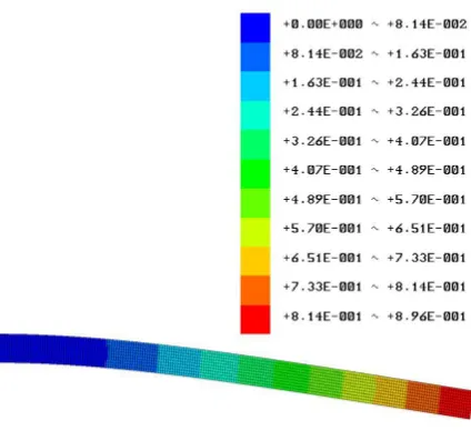
The displacement field of the quadratic hexahedron model is shown in Fig. 4. The values of the maximum total displacement are summarized in Table 2.

Table 2. Results of the maximum displacement de-pending on the element type and number of elements

Element type Number of _{elements Σ} i biR



[N] displacement [mm]Maximum Linear hexahedron 20000 1540.17 0.891 Quadratic hexahedron 20000 1540.17 0.896 Linear tetrahedron 86011 1540.17 0.871 Quadratic tetrahedron 86011 1540.17 0.896

The quality of the calculated maximum total displacements depends on the element type and on the number of finite elements.

Fig. 4. Total displacement of the cantilever beam

5 DISCUSSION

Using the factorization-based method for the calculation of weight forces within the finite element analysis can lead to a noticeable reduction of the computation time, as shown in Section 3.

However, this approach is not limited to the calculation of weight forces but can be generalized as follows:

f r s t dV I X

V k ijk ijk

n

j n

i n

( , , ) ,

∫∫∫

=

∑

∑

∑

⋅

= = =1 1 1

(18)

where Iijk is defined as:

I_ijk f r s t H drdsdt_ijk

r s t

=

_∫∫∫

( , , ) .

( , , )

(19)

If the integrand f (r, s, t) is solely a function of the natural coordinates and independent of the Cartesian node coordinates, these integrals Iijk can be calculated

in advance. This may lead to a noticeable advantage in computation time under the following circumstances: 1) The calculation of the Iijk is not included in the

computation time, because the calculation can be done before the program runtime.

2) There are many volume integrals of the same type to be solved so that it is possible to reuse the integrals Iijk.

In the context of the finite element analysis, the volume integral of the mass matrix [5] or other body forces, such as the centrifugal force [12], fulfil both criteria.

As shown in Section 3, the application of the factorization-based method can lead to a noticeable reduction of the computation during the calculation of the nodal weight forces of a quadratic tetrahedron

element. In general, the ratio of computation times of the standard approach using Gaussian quadrature and of the factorization-based method depends on several aspects:

1) The complexity of the function f: The more complex the function f, the more CPU-intensive its evaluation at the supporting points. For instance, a high polynomial degree of the integrand requires a high integration order to obtain an exact numerical integration of the volume integral, which affects the computational effort and time of the Gaussian integration method. In contrast, the factorization-based method is not affected, because the actual integration of f is not performed during the program runtime. Therefore, a high complexity of the function f leads to a high ratio of computation times.

2) The element type: In general, a higher polynomial degree of the shape functions requires a higher integration order to ensure exact numerical integration regarding the Jacobian determinant. Therefore, the computing effort for the Gaussian quadrature increases. At the same time, the computation effort of the factorization-based method also grows, since a finite element of higher order has a larger number of nodes n. These competing factors must be considered in terms of computational effort and time.

3) The software implementation: The way both integration methods are implemented into the finite element software can affect the ratio of computation times. In this context, the factorization-based method provides the advantage that no Gaussian quadrature needs to be implemented.

The advantage of the factorization-based method over the standard approach will therefore differ for different cases of application. Each case must be considered individually.

6 CONCLUSIONS

The consideration of body forces, such as the weight force, is crucial for the stress analysis of many technical applications.

In this paper, we introduced an efficient approach for the exact calculation of the resultant weight force on the nodes of three-dimensional continuum elements.

Cartesian node coordinates. The original volume integral can thereby be split up into a sum of integrals independent of the Cartesian node coordinates. The node coordinates are considered by prefactors during the summation. Since these integrals are solely dependent on the shape functions, they are specific for the element type, such as the quadratic tetrahedron. Consequently, the integrals need to be calculated only once and the resultant numerical values can be tabulated hard coded in the finite element program.

No Gaussian quadrature needs to be performed for the calculation of the resultant nodal weight forces during the finite element analysis, which reduces the computational effort and time.

Furthermore, an exact evaluation of the introduced integrals can be performed in advance leading to an exact calculation of the nodal forces without affecting the computation time of the finite element program.

As demonstrated by a comparative calculation in Section 4, the factorization-based method can be faster than the standard approach using Gaussian quadrature with the same accuracy.

The introduced method is not limited to the calculation of weight forces but can also be applied to calculate the mass matrix and other body forces within the FEA. Furthermore, the method can be generalized to be applicable to two-dimensional continuum elements.

7 REFERENCES

[1] Zienkiewicz, O.C., Taylor, R.L., Zhu, J.Z. (2005). The Finite

Element Method – Its Basis and Fundamentals. Elsevier Ltd.,

Oxford.

[2] Bathe, K.J. (2002). Finite-Elemente-Methoden. Springer-Verlag, Berlin, Heidelberg, DOI:10.1007/978-3-642-56078-1. [3] Rieg, F., Hackenschmidt, R., Alber-Laukant, B. (2014). Finite

Element Analysis for Engineers. Hanser, München.

[4] Lynch, D.R. (2005). Numerical Partial Differential Equations

for Environmental Scientists and Engineers. Springer, New

York.

[5] Liu, G.R., Quek, S.S. (2014). The Finite Element Method – A

Practical Course. Butterworth-Heinemann, Oxford.

[6] Krishnamoorthy, C.S. (1994). Finite Element Analysis: Theory

and Programming. McGraw Hill Education, New Delhi.

[7] Hussain, F., Karim, M.S., Ahamad, R. (2012). Appropriate Gaussian quadrature formulae for triangles. International

Journal of Applied Mathematics and Computation, vol. 4, no.

1, p. 24-38.

[8] Reddy, C.T., Shippy, D.J. (1981). Alternative integration formulae for triangular finite elements. International Journal

for Numerical Methods in Engineering, vol. 17, no. 1, p.

133-139, DOI:10.1002/nme.1620170111.

[9] Schwarz, H.R., Köckler, N. (2011). Numerische Mathematik. Vieweg+Teubner, Wiesbaden

[10] Bronstein, I., Semendjajew, K., Musiol, G., Mühlig, H. (2013).

Taschenbuch der Mathematik. Europa-Lehrmittel,

Haan-Gruiten.

[11] Grote, K.-H., Feldhusen, J. (2014). DUBBLE Taschenbuch für

den Maschinenbau. Springer, Berlin, Heidelberg.

[12] Logan, D.L. (2007). A First Course in the Finite Element