CFD-DEM Investigation on van der Waals Force in Gas-Solid Bubbling Fluidized Beds

(1)

93 S.M. Okhovat-Alavian et al. / Journal of Chemical and Petroleum Engineering, 52 (1), June 2018 / 93-105

CFD-DEM Investigation on van der Waals Force

in Gas-Solid Bubbling Fluidized Beds

S.M. Okhovat-Alavian

1

_{, H.R. Norouzi}

2

**_{and N. Mostoufi*}**

1

1. Process Design and Simulation Research Center, School of Chemical Engineering, College of Engineering, University of Tehran, P.O. Box 11155-4563, Tehran, Iran.

2. Depatment of Chemical Engineering, Amirkabir University of Technology (Tehran Polytechnic), PO Box: 15875-4413, Hafez 424, Tehran, Iran.

(Received 19 April 2018, Accepted 30 May 2018) [DOI: 10.22059/jchpe.2018.256180.1230]

Abstract

Effect of interparticle force on the hydrodynamic of gas-solid fluid -ized beds was investigated using the combined method of computa-tional fluid dynamics and discrete element method (CFD-DEM). The cohesive force between particles was considered to follow the van der Waals form. The model was validated by experimental results in terms of bed voidage distribution and Eulerian solid velocity field. The re -sults revealed that the incorporated model can satisfactorily predict the hydrodynamics of the fluidized bed in the presence of interparticle forces. Effect of interparticle force on bubble rise characteristics such bubble stability, bubbles diameter and bubble velocity, was investigat-ed. It was shown that emulsion voidage increases with the interpar-ticle force in the bed and it can hold more gas inside its structures. In addition by increasing interparticle force, the bubble size and bubble rise velocity increase while the average velocity of particles decreases.

Keywords

Discrete element method; Interparticle forces; Hydrodynamics; Bubble;

Fluidization.

Introduction

1

* Corresponding Author.

Tel.: (+98-21) 6696-7781 Fax: (+98-21) 6695-7784

Email: mostoufi@ut.ac.ir (N. Mostoufi)

1. Introduction

as–solid fluidized beds are used in a variety of industrial processes due to uniform bed temperature, high mass and heat transfer rates and suitability for large-scale operations [1]. Based on their fluidization behavior, powders are categorized into four groups according to their size and density, called Geldart A, B, C and D [10].

However, experimental evidences indicate that

(2)

and then group C. Increase in IPFs increases min-imum fluidization velocity, transition velocity from bubbling to turbulent fluidization, the ten-dency of gas passing through the emulsion and bubble size [29].

Although the experimental measurements have provided proper understanding of hydrodynamic changes of gas-solid flows in the presence of IPFs. However, much is to be known about particle-scale phenomena and the mechanisms governing the hydrodynamics of fluidization (e.g., change in the minimum fluidization velocity, change in bubble diameter, etc.) in the presence of IPFs, which can hardly be obtained through experi-ment. Therefore, numerical simulations can be used to overcome the difficulties of experiments and to obtain detailed information about such phenomena. Among various approaches for mod-eling fluidized beds, the combination of discrete element method (DEM) [6] and computational fluid dynamics (CFD) [34] is among the promising ones. In this approach, particles form the discrete phase and each individual particle is tracked in time and space by integrating the Lagrangian equation of motion while gas is assumed to be the continuum phase and its flow characteristics are obtained by solving the volume averaged Navier-Stokes equation. Yu and Xu [41] and Ye et al. [40] used the CFD-DEM technique and included the van der Waals force to study the fluidization be-havior of group A particles. They found that the regime is homogeneous when the van der Waals force is relatively weak. Rhodes et al. [25] added a cohesive force between particles in their simula-tions and demonstrated that the fluidization characteristics of Geldart group B or D particles change to Geldart Group A. The most important change in this case was observing non-bubbling fluidization for gas velocities between the mini-mum fluidization and the minimini-mum bubbling which are the group A fluidization characteristics. Pandit et al. [23] studied the effect of van der Waals force on formation and characteristics of bubbles and found that in the presence of high level of van der Waals force, not only does the bubble formation process require a higher air velocity for its initiation, but also it is slower when compared to the case with no van der Waals force. Kaboyashi et al. [14-16] also showed that the bed pressure drop hysteresis during flu-idization and defluflu-idization processes can be ob-served and the spring stiffness constant used in

the DEM model has a significant influence on the adhesive behavior of particle to the wall.

Effect of IPFs on bubble dynamics (i.e., bubble diameter and rise velocity in a gas fluidized bed) has not been studies properly yet. To fill this gap in the fluidization process, a CFD–DEM study was conducted in this work to describe the character-istics of bubbles in a two-dimensional fluidized bed at different level of cohesive interparticle force. The results of probability density distribu-tion of the instantaneous local bed voidage and

volume-averaged solid velocity field were

com-pared with experimental results available in liter-ature to validate the model. The influences of IPFs on the bubble characteristics, stability, diameter and velocity were then investigated.

2. Numerical Model

In the CFD-DEM approach, particles are assumed to be the discrete phase and gas is assumed to be the continuum phase. For the contacts between particles, the soft-sphere approach was used in which particles can overlap partially, hence, par-ticles can have multiple contacts [6]. The gas phase motion is described by the volume-averaged Navier-Stokes equation over an Euleri-an mesh. The coupling between phases is done through inter-phase momentum transfer (i.e., drag and pressure gradient forces) and gas vol-ume fraction. Since the density of solid particle is much greater than the density of gas, the buoyant force acting on each particle was ignored. The governing equations are described in the follow-ings.

2.1. Governing equations for particles

Translational and rotational motions are consid-ered for each particle. The translational motion of

each spherical particle i, described by the

New-ton’s second law of motion, and the rotational motion are given by [37]:

2

d, 2

1

c

n _c i

i

ij i

i i g

j

dv

d r

m

f

dt





uv



uv



uv

₍₁₎

1 t

k _t

i _ij

i

j d

I M

dt







uuv ₍₂₎

4

particle was ignored. The governing

equations are described in the followings.

2.1. Governing equations for particles

Translational and rotational motions are

considered for each particle. The

translational motion of each spherical

particle

i

, described by the

Newton’s

second

law of motion, and the rotational motion are

given by [37]:

2

d, 2

1

c

n _c i

i

ij i vdW

i i g

j

dv

d r

m

f

dt







1

t

k _t i

ij i

j

d

I

M

dt







₍₂₎

The terms on the right-hand side of Eq. (1)

are sum of contact forces, fluid-drag force,

gravitational force and sum of cohesive

forces, respectively. The contact forces

between particle-particle and particle-wall

(wall as particle

j

with infinity radius) are

composed of normal

f

ijn

and tangential

f

tij

components. The cohesive force consists of

particle-particle and particle

–

wall cohesive

forces. The expressions used to calculate the

forces and torques are given in Table 1.

2.2. Cohesive force

In this study, the cohesive force between

two particles and between particles and wall,

was assumed to follow the van der Waals

form. A particle may interact with its

surrounding particles (

n

k

particles) via the

van der Waals force. In this work, the Verlet

list was employed to detect interparticle

interactions and a cut-off radius was

considered for the van der Waals force. Fig.

1 shows the schematic of the Verlet list of a

target particle.

Figure 1. The Verlet list of a target particle i

According to this approach, all particles

around the target particle that lie within a

sphere with radius

R

cut-off

are considered in

the Verlet list of the target particle. Since

particles move a very short distance in each

integration time step, list remains unchanged

in several time steps. This prevents

redundant updates of the Verlet list during

the simulation which is the main advantage

of this method. In the present work, the

cut-off radius,

R

cut-off

, for the target particle was

assumed to be the distance beyond which

Rcut-off

i

Target particle, i Particles in Verlet list, k Particles out of Verlet list

4 particle was ignored. The governing equations are described in the followings.

2.1. Governing equations for particles

Translational and rotational motions are considered for each particle. The translational motion of each spherical particlei, described by the Newton’ssecond law of motion, and the rotational motion are given by [37]:

2

d, 2

1 c

n _c i

i

ij i vdW

i i g

j

dv

d r

m

f

dt







1 t

k _t

i _ij

i

j d

I M

dt







₍₂₎

The terms on the right-hand side of Eq. (1) are sum of contact forces, fluid-drag force, gravitational force and sum of cohesive forces, respectively. The contact forces between particle-particle and particle-wall (wall as particle j with infinity radius) are composed of normal f ijn and tangential f tij

components. The cohesive force consists of particle-particle and particle–wall cohesive forces. The expressions used to calculate the forces and torques are given in Table 1.

2.2. Cohesive force

In this study, the cohesive force between two particles and between particles and wall, was assumed to follow the van der Waals

form. A particle may interact with its surrounding particles (nk particles) via the van der Waals force. In this work, the Verlet list was employed to detect interparticle interactions and a cut-off radius was considered for the van der Waals force. Fig. 1 shows the schematic of the Verlet list of a target particle.

According to this approach, all particles around the target particle that lie within a sphere with radius Rcut-off are considered in the Verlet list of the target particle. Since particles move a very short distance in each integration time step, list remains unchanged in several time steps. This prevents redundant updates of the Verlet list during the simulation which is the main advantage of this method. In the present work, the cut-off radius, Rcut-off, for the target particle was assumed to be the distance beyond which

Rcut-off i

(3)

The terms on the right-hand side of Eq. (1) are sum of contact forces, fluid-drag force, gravita-tional force and sum of cohesive forces, respec-tively. The contact forces between

particle-particleandparticle-wall(wallasparticlejwith

infinity radius) are composed of normal

f

uv

nij and

tangential

f

uv

tij components. The cohesive force

consists of particle-particle and particle–wall co-hesive forces. The expressions used to calculate the forces and torques are given in Table 1.

2.2. Cohesive force

In this study, the cohesive force between two par-ticles and between parpar-ticles and wall, was as-sumed to follow the van der Waals form. A

parti-cle may interact with its surrounding partiparti-cles (nk

particles) via the van der Waals force. In this work, the Verlet list was employed to detect in-terparticle interactions and a cut-off radius was considered for the van der Waals force. Fig. 1 shows the schematic of the Verlet list of a target particle.

According to this approach, all particles around the target particle that lie within a sphere with radius Rcut-off are considered in the Verlet list of

the target particle. Since particles move a very short distance in each integration time step, list remains unchanged in several time steps. This prevents redundant updates of the Verlet list dur-ing the simulation which is the main advantage of this method. In the present work, the cut-off radi-us, Rcut-off, for the target particle was assumed to

be the distance beyond which the van der Waals

force becomes less than 5% of weight of the par-ticle.

As shown in Table 1, the van der Waals force is a function of the surface distance between particles or between particle and wall. When the particles or particle and wall are in contact, an unrealistic large van der Waals force would be obtained from the equations of Table 1. To solve this problem, a minimum separation distance of 0.4 nm is con-sidered between particles and particle and wall [16, 33].

2.3. Governing equations for fluid

The volume-averaged continuity and Navier– Stokes are [2]:



f



_.

_

_

₀

f

u

t





 





v

(3)





_

_

 

. . f f fp f f u uu t

p F g









           v vv uv (4)

The term

F

fp

uv

represents the average momentum exchange term between the solid and gas phases:

, c d i fp i C

k f

F

V





uv

(5)

where Vc is volume of the fluid cell.

2.4. Coupling

Equations of gas and the solid phases are coupled through porosity and fluid–particle interaction force,

F

fp

uv

. Various schemes for coupling the in-terphase momentum interactions can be consid-ered as reviewed by Feng et al. [9]. According to their recommendation, the forces acting on each particle should be computed through the fluid volume fraction and local fluid velocity in each fluid cell. The obtained forces are substituted in the equation of motion, Eq. (1), for each particle and then integrated over time to calculate new velocities and positions of particles. The particle– fluid interaction force in each fluid cell is then calculated by Eq. (5). More information and

ex-Rcut-off i

5

the van der Waals force becomes less than

5% of weight of the particle.

As shown in Table 1, the van der Waals

force is a function of the surface distance

between particles or between particle and

wall. When the particles or particle and wall

are in contact, an unrealistic large van der

Waals force would be obtained from the

equations of Table 1. To solve this problem,

a minimum separation distance of 0.4 nm is

considered between particles and particle

and wall [16, 33].

2.3. Governing equations for fluid

The volume-averaged continuity and

Navier

–

Stokes are [2]:



f



_.

_

_

₀

f

u

t





 





(3)





_

_

 

p F g









          

(4)

The term

F

fp

_{represents the average}

momentum exchange term between the solid

and gas phases:

,

c _{d i}

fp i C

k f

F

V





(5)

where V

c

is volume of the fluid cell.

2.4. Coupling

Equations of gas and the solid phases are

coupled through porosity and fluid

–

particle

interaction force,

F

fp

_{. Various schemes for}

coupling the interphase momentum

interactions can be considered as reviewed

by Feng et al. [9]. According to their

recommendation, the forces acting on each

particle should be computed through the

fluid volume fraction and local fluid velocity

in each fluid cell. The obtained forces are

substituted in the equation of motion, Eq.

(1), for each particle and then integrated

over time to calculate new velocities and

positions of particles. The particle

–

fluid

interaction force in each fluid cell is then

calculated by Eq. (5). More information and

explanation about the coupling process are

provided by Norouzi et al. [22].

The solid volume fraction is calculated

through the volume occupied by the

particles in each fluid cell:

3 ,

1

kc i

D cell p i i C

V







 



₍₆₎

Where



celli

_and

_V

_p,i

_{are fractional volume of}

particle

i

presenting in each cell and volume

of that particle, respectively. In the present

work, the size of fluid cell was larger than

the particle size (at least 4 times) but smaller

than the macroscopic structures in the bed

(i.e., bubbles). The SIMPLE (Semi-Implicit

Method for Pressure-Linked Equations)

5

the van der Waals force becomes less than

5% of weight of the particle.

As shown in Table 1, the van der Waals

force is a function of the surface distance

between particles or between particle and

wall. When the particles or particle and wall

are in contact, an unrealistic large van der

Waals force would be obtained from the

equations of Table 1. To solve this problem,

a minimum separation distance of 0.4 nm is

considered between particles and particle

and wall [16, 33].

2.3. Governing equations for fluid

The volume-averaged continuity and

Navier

–

Stokes are [2]:



f



_.

_

_

₀

f

u

t





 





(3)





_

_

 

p F g









          

(4)

The term

F

fp

_{represents the average}

momentum exchange term between the solid

and gas phases:

,

c _{d i}

fp i C

k f

F

V





(5)

where V

c

is volume of the fluid cell.

2.4. Coupling

Equations of gas and the solid phases are

coupled through porosity and fluid

–

particle

interaction force,

F

fp

_{. Various schemes for}

coupling the interphase momentum

interactions can be considered as reviewed

by Feng et al. [9]. According to their

recommendation, the forces acting on each

particle should be computed through the

fluid volume fraction and local fluid velocity

in each fluid cell. The obtained forces are

substituted in the equation of motion, Eq.

(1), for each particle and then integrated

over time to calculate new velocities and

positions of particles. The particle

–

fluid

interaction force in each fluid cell is then

calculated by Eq. (5). More information and

explanation about the coupling process are

provided by Norouzi et al. [22].

The solid volume fraction is calculated

through the volume occupied by the

particles in each fluid cell:

3 ,

1

kc i

D cell p i i C

V







 



₍₆₎

Where



celli

_and

_V

_p,i

_{are fractional volume of}

particle

i

presenting in each cell and volume

of that particle, respectively. In the present

work, the size of fluid cell was larger than

the particle size (at least 4 times) but smaller

than the macroscopic structures in the bed

(i.e., bubbles). The SIMPLE (Semi-Implicit

Method for Pressure-Linked Equations)

5

the van der Waals force becomes less than

5% of weight of the particle.

As shown in Table 1, the van der Waals

force is a function of the surface distance

between particles or between particle and

wall. When the particles or particle and wall

are in contact, an unrealistic large van der

Waals force would be obtained from the

equations of Table 1. To solve this problem,

a minimum separation distance of 0.4 nm is

considered between particles and particle

and wall [16, 33].

2.3. Governing equations for fluid

The volume-averaged continuity and

Navier

–

Stokes are [2]:



f



_.

_

_

₀

f

u

t





 





(3)





_

_

 

p F g









          

(4)

The term

F

fp

_{represents the average}

momentum exchange term between the solid

and gas phases:

,

c _{d i}

fp i C

k f

F

V





(5)

where V

c

is volume of the fluid cell.

2.4. Coupling

Equations of gas and the solid phases are

coupled through porosity and fluid

–

particle

interaction force,

F

fp

_{. Various schemes for}

coupling the interphase momentum

interactions can be considered as reviewed

by Feng et al. [9]. According to their

recommendation, the forces acting on each

particle should be computed through the

fluid volume fraction and local fluid velocity

in each fluid cell. The obtained forces are

substituted in the equation of motion, Eq.

(1), for each particle and then integrated

over time to calculate new velocities and

positions of particles. The particle

–

fluid

interaction force in each fluid cell is then

calculated by Eq. (5). More information and

explanation about the coupling process are

provided by Norouzi et al. [22].

The solid volume fraction is calculated

through the volume occupied by the

particles in each fluid cell:

3 ,

1

kc i

D cell p i i C

V







 



₍₆₎

Where



celli

_and

_V

_p,i

_{are fractional volume of}

particle

i

presenting in each cell and volume

of that particle, respectively. In the present

work, the size of fluid cell was larger than

the particle size (at least 4 times) but smaller

than the macroscopic structures in the bed

(i.e., bubbles). The SIMPLE (Semi-Implicit

Method for Pressure-Linked Equations)

5

the van der Waals force becomes less than

5% of weight of the particle.

As shown in Table 1, the van der Waals

force is a function of the surface distance

between particles or between particle and

wall. When the particles or particle and wall

are in contact, an unrealistic large van der

Waals force would be obtained from the

equations of Table 1. To solve this problem,

a minimum separation distance of 0.4 nm is

considered between particles and particle

and wall [16, 33].

2.3. Governing equations for fluid

The volume-averaged continuity and

Navier

–

Stokes are [2]:



f



_.

_

_

₀

f

u

t





 





(3)





_

_

 

p F g









          

(4)

The term

F

fp

_{represents the average}

momentum exchange term between the solid

and gas phases:

, c d i fp i C

k f

F

V





(5)

where V

c

is volume of the fluid cell.

2.4. Coupling

Equations of gas and the solid phases are

coupled through porosity and fluid

–

particle

interaction force,

F

fp

_{. Various schemes for}

coupling the interphase momentum

interactions can be considered as reviewed

by Feng et al. [9]. According to their

recommendation, the forces acting on each

particle should be computed through the

fluid volume fraction and local fluid velocity

in each fluid cell. The obtained forces are

substituted in the equation of motion, Eq.

(1), for each particle and then integrated

over time to calculate new velocities and

positions of particles. The particle

–

fluid

interaction force in each fluid cell is then

calculated by Eq. (5). More information and

explanation about the coupling process are

provided by Norouzi et al. [22].

The solid volume fraction is calculated

through the volume occupied by the

particles in each fluid cell:

3 ,

1

kc i

D cell p i i C

V







 



₍₆₎

Where



celli

_and

_V

_p,i

_{are fractional volume of}

particle

i

presenting in each cell and volume

of that particle, respectively. In the present

work, the size of fluid cell was larger than

the particle size (at least 4 times) but smaller

than the macroscopic structures in the bed

(i.e., bubbles). The SIMPLE (Semi-Implicit

Method for Pressure-Linked Equations)

4

particle was ignored. The governing

equations are described in the followings.

2.1. Governing equations for particles

Translational and rotational motions are

considered for each particle. The

translational motion of each spherical

particle

i

, described by the

Newton’s

second

law of motion, and the rotational motion are

given by [37]:

2 d, 2 1 c n _c i i

ij i vdW

i i g

j

dv

d r

m

f

dt







1 t k _t i ij i j

d

I

M

dt







₍₂₎

The terms on the right-hand side of Eq. (1)

are sum of contact forces, fluid-drag force,

gravitational force and sum of cohesive

forces, respectively. The contact forces

between particle-particle and particle-wall

(wall as particle

j

with infinity radius) are

composed of normal

f

ijn

and tangential

f

tij

components. The cohesive force consists of

particle-particle and particle

–

wall cohesive

forces. The expressions used to calculate the

forces and torques are given in Table 1.

2.2. Cohesive force

In this study, the cohesive force between

two particles and between particles and wall,

was assumed to follow the van der Waals

form. A particle may interact with its

surrounding particles (

n

k

particles) via the

van der Waals force. In this work, the Verlet

list was employed to detect interparticle

interactions and a cut-off radius was

considered for the van der Waals force. Fig.

1 shows the schematic of the Verlet list of a

target particle.

According to this approach, all particles

around the target particle that lie within a

sphere with radius

R

cut-off

are considered in

the Verlet list of the target particle. Since

particles move a very short distance in each

integration time step, list remains unchanged

in several time steps. This prevents

redundant updates of the Verlet list during

the simulation which is the main advantage

of this method. In the present work, the

cut-off radius,

R

cut-off

, for the target particle was

assumed to be the distance beyond which

Rcut-off

i

4

particle was ignored. The governing

equations are described in the followings.

2.1. Governing equations for particles

Translational and rotational motions are

considered for each particle. The

translational motion of each spherical

particle

i

, described by the

Newton’s

second

law of motion, and the rotational motion are

given by [37]:

2 d, 2 1 c n _c i i

ij i vdW

i i g

j

dv

d r

m

f

dt







1 t k _t i _ij i j

d

I

M

dt







₍₂₎

The terms on the right-hand side of Eq. (1)

are sum of contact forces, fluid-drag force,

gravitational force and sum of cohesive

forces, respectively. The contact forces

between particle-particle and particle-wall

(wall as particle

j

with infinity radius) are

composed of normal

f

ijn

and tangential

f

tij

components. The cohesive force consists of

particle-particle and particle

–

wall cohesive

forces. The expressions used to calculate the

forces and torques are given in Table 1.

2.2. Cohesive force

In this study, the cohesive force between

two particles and between particles and wall,

was assumed to follow the van der Waals

form. A particle may interact with its

surrounding particles (

n

k

particles) via the

van der Waals force. In this work, the Verlet

list was employed to detect interparticle

interactions and a cut-off radius was

considered for the van der Waals force. Fig.

1 shows the schematic of the Verlet list of a

target particle.

According to this approach, all particles

around the target particle that lie within a

sphere with radius

R

cut-off

are considered in

the Verlet list of the target particle. Since

particles move a very short distance in each

integration time step, list remains unchanged

in several time steps. This prevents

redundant updates of the Verlet list during

the simulation which is the main advantage

of this method. In the present work, the

cut-off radius,

R

cut-off

, for the target particle was

assumed to be the distance beyond which

Rcut-off

i

(4)

planation about the coupling process are provid-ed by Norouzi et al. [22].

The solid volume fraction is calculated through the volume occupied by the particles in each fluid cell:

3 ,

1

kc i

D cell p i

i C

V







 



₍₆₎

Where



celli _and_V_p,i_{are fractional volume of}

par-ticle i presenting in each cell and volume of that particle, respectively. In the present work, the size of fluid cell was larger than the particle size

(at least 4 times) but smaller than the macroscop-ic structures in the bed (i.e., bubbles). The SIM-PLE (Semi-Implicit Method for Pressure-Linked Equations) algorithm [24] was applied to solve the gas phase equations.

The first order up-wind scheme was utilized for the convection terms. The Eulerian cell size was 2.3 mm (4 times greater than the particle diame-ter). In the case of the fluid velocity, the no-slip boundary condition was used to the walls and the fully developed condition to the exit at the top. An in-house code written in FORTRAN was used for the simulations [13].

Table 1. Relations for evaluating various forces acting on particle i.

Force Type Symbol Formula

contact forces [17] normal n ij

f

uv



(

k

_{n n}



)

n

uuv

_ij



(



_i

V

uv uv uv

r ij,

. )

n n

ij ij

tangential t ij

f

uv





,

min

n

,

t

ij _{t t} ij ij _i t ij

t

f

k t



t

V

















_



_







uv

v

uv

torque - t

ij

M

uuv

R

uv uv

i



f

tij

gravity -

,

g i

f

uv

m g

i

van der Waals forces [7] particle-particle

, vdw ik

f

uv

2

24

p ij

d

H

h

particle-wall ,

vdw i w

f



uv

2

12

p iw

d

H

h

fluid drag force [8]

,

d i

f

uv

f

ˆ

d i,



3 

d

p i,

 

f

(

u v



i

)

v v

,

ˆ

_Re

24

d

d i

C

p

f

_

_



10

3.7 0.65exp( 0.5(1.5 log Re ))

_p







1 ₂ 2

(0.63 4.8Re

)

d p

C







,

ˆ

,

i

,

i j

,Re

f p i i

i j i ij r ij i j _ij _p

i i j f

d

u v

R

r

r n

V

R





 





 















v v

uv

uv uv

uv

v

v uv

uv

uv uv

uv

uv uv

5

the van der Waals force becomes less than

5% of weight of the particle.

As shown in Table 1, the van der Waals

force is a function of the surface distance

between particles or between particle and

wall. When the particles or particle and wall

are in contact, an unrealistic large van der

Waals force would be obtained from the

equations of Table 1. To solve this problem,

a minimum separation distance of 0.4 nm is

considered between particles and particle

and wall [16, 33].

2.3. Governing equations for fluid

The volume-averaged continuity and

Navier

–

Stokes are [2]:



f



_.

_

_

₀

f

u

t





 





(3)





_

_

 

p F g









          

(4)

The term

F

fp

_{represents the average}

momentum exchange term between the solid

and gas phases:

, c d i fp i C

k f

F

V





(5)

where V

c

is volume of the fluid cell.

2.4. Coupling

Equations of gas and the solid phases are

coupled through porosity and fluid

–

particle

interaction force,

F

fp

_{. Various schemes for}

coupling the interphase momentum

interactions can be considered as reviewed

by Feng et al. [9]. According to their

recommendation, the forces acting on each

particle should be computed through the

fluid volume fraction and local fluid velocity

in each fluid cell. The obtained forces are

substituted in the equation of motion, Eq.

(1), for each particle and then integrated

over time to calculate new velocities and

positions of particles. The particle

–

fluid

interaction force in each fluid cell is then

calculated by Eq. (5). More information and

explanation about the coupling process are

provided by Norouzi et al. [22].

The solid volume fraction is calculated

through the volume occupied by the

particles in each fluid cell:

3 ,

1

kc i

D cell p i

i C

V







 



₍₆₎

Where



celli

_and

_V

_p,i

_{are fractional volume of}

particle

i

presenting in each cell and volume

of that particle, respectively. In the present

work, the size of fluid cell was larger than

the particle size (at least 4 times) but smaller

than the macroscopic structures in the bed

(i.e., bubbles). The SIMPLE (Semi-Implicit

Method for Pressure-Linked Equations)

planation about the coupling process are provid-ed by Norouzi et al. [22].

The solid volume fraction is calculated through the volume occupied by the particles in each fluid cell:

3 ,

1

kc i

D cell p i

i C

V







 



₍₆₎

Where



celli _and_V_p,i_{are fractional volume of}

par-ticle i presenting in each cell and volume of that particle, respectively. In the present work, the size of fluid cell was larger than the particle size

(at least 4 times) but smaller than the macroscop-ic structures in the bed (i.e., bubbles). The SIM-PLE (Semi-Implicit Method for Pressure-Linked Equations) algorithm [24] was applied to solve the gas phase equations.

The first order up-wind scheme was utilized for the convection terms. The Eulerian cell size was 2.3 mm (4 times greater than the particle diame-ter). In the case of the fluid velocity, the no-slip boundary condition was used to the walls and the fully developed condition to the exit at the top. An in-house code written in FORTRAN was used for the simulations [13].

contact forces [17] normal n ij

f

uv



(

k

n n



)

n

ij



(



i

V

r ij,

. )

n n

ij ij

uuv

uv uv uv

tangential t ij

f

uv





,

min

n

,

t

ij _{t t} ij ij _i t ij

t

f

k t



t

V

















_



_







uv

v

uv

torque - t

ij

M

uuv

t

i ij

R

uv uv



f

gravity -

,

g i

f

uv

m g

i

van der Waals forces [7] particle-particle

, vdw ik

f

uv

2

24

p ij

d

H

h

particle-wall ,

vdw i w

f



uv

2

12

p iw

d

H

h

,

d i

f

uv

, ,

ˆ

_{d i}

₃

_{p i} _f

₍

_i

₎

f





d

 

u v

v v



,

ˆ

_Re

24

d

d i

C

p

f

_

_



10

3.7 0.65exp( 0.5(1.5 log Re ))

_p







1₂ ₂

(0.63 4.8Re

)

d p

C







,

ˆ

,

i

,

i j

,Re

f p i i

i i j f

d

u v

R

r

r n

V

R





 





 















v v

uv

uv uv

uv

v

v uv

uv

uv uv

uv

uv uv

6 algorithm [24] was applied to solve the gas phase equations.

The first order up-wind scheme was utilized for the convection terms. The Eulerian cell size was 2.3 mm (4 times greater than the particle diameter). In the case of the fluid

velocity, the no-slip boundary condition was used to the walls and the fully developed condition to the exit at the top. An in-house code written in FORTRAN was used for the simulations [13].

contact forces [17] normal n

ij

f (k_{n n}



)n_ij (



_iV r ij, . )n nij ij

tangential t

ij

f





,

min n_ij , t

ij ij t ij

t t i

t

f k t



t V









 

_ _ 

 

torque - t

ij

M Rif tij

gravity -

_f

_{g i}_,

m g

i

van der Waals forces [7] particle-particle , vdw ik

f

2 24 p ij d H h

particle-wall

_f

_{vdw i w}_, 

2 12 p iw d H h

_f

_{d i}_, ˆ_, ₃ _, ₍ _i₎

d i p i f

f 



d

 

u v

,

ˆ _Re

24d

d i C p

f _ _

10

3.7 0.65exp( 0.5(1.5 log Re ))

p







1 ₂ 2

(0.63 4.8Re )

d p

C   

,

, ˆ

, i , , i j ,Re f p i i

i i j f

d u v

R

R r r n V V V

(5)

Table 2. Experimental and simulation conditions and parameters

3. Experimental Data and Simulation

Conditions

3.1. Experimental data

In order to validate the model, the numerical re-sults probability density distribution of the in-stantaneous local bed voidage and

volume-averaged solid velocity fieldwere compared with

experimental results of Shabanian and Chaouki [28, 29] at various values of IPF. Shabanian and Chaouki [2011] applied a polymer coating ap-proach to increase and adjust the level of IPFs in a gas–solid fluidized bed. Their method was based on coating spherical inert particles with a poly-mer with a low glass transition temperature. In the present work, the data obtained by Shabanian and Chaouki [28,29] were utilized for validation of the model. Uncoated (fresh) and coated sugar beads (dp = 580 µm, ρp = 1556 kg/m3) were sepa-rately used in the fluidized bed at various operat-ing temperatures to investigate the effect of IPF on the hydrodynamics of a gas–solid fluidized bed. The initial bed height was 26 cm (H/Dc≈1.70), i.e., 4.0 kg of powder. The

magni-tude of IPF was controlled by temperature of the inlet air. The bed temperature was changed near and slightly above the glass transition

tempera-ture of the polymer, between 20 and 40 _{C. For}

simplicity, the tests at various operating tempera-tures are called in shortened form of SB20, CSB30, CSB35

and CSB40, which stand for uncoated sugar beads at 20 _{C and coated sugar beads at 30, 35, and 40}

_{C, respectively. Before the work of Shabanian}

and Chaouki [31], Buoffard et al. [4] also applied the same approach and material. They estimated the adhesion energy for the coated polymer by measuring the pull-off force. Their results illus-trated that the magnitude of IPFs is in the same range of van der Waals force.

3.2. Simulation conditions

A rectangular bed filled with particles of the same in size and density in the experiments and air as the fluidizing gas, were considered in the simula-tions. It is worth mentioning that the number of particles in experiments was very large such that its simulation is not feasible with the existing computational resources. To overcome this prob-lem and reduce the simulation time, number of particles was reduced by considering a smaller bed. The same aspect ratio L/Dc =1.7 was

consid-ered in both simulations and experiments, based on which the bed width in simulations was con-sidered to be 5.04 cm. All the needed data (pres-sure and voidage) were recorded from the center of the bed in order to avoid the wall effect. The properties of bed, particles and air are listed in Table 2. All the simulations were continued for 15 s in real time.

Simulation

Particles Gas Bed

Shape Spherical Fluid Air Width (m) 0.0504

Number of particles 155000 CFD cell size (mm2₎ _{2.4 × 2.4} _{Height (m)} _0.4

Particle diameter (m) 0.00058 Viscosity (kg/m.s) 1.8510-5 _{Thickness (m)} _0.0058

Density (kg/m3₎ ₁₅₅₆ _{Bed distributor} _{Porous plate}

Initial height (m) 0.085 Pressure (MPa) 0.1 Spring constant (N/m) 1000 Density (kg/m3₎ _1.2

Sliding friction coefficient 0.3 Umf (m/s) 0.16

Restitution coefficient 0.9 Superficial velocity (m/s) 0.35, 0.6, 0.9 Time step (s) 0.510-5 _{Time step (s)} _0.5_₁₀-4

Experiment

Particles Gas Bed

Shape Spherical Fluid Air radius (m) 0.152

Diameter (μm) 580 Viscosity (kg/m.s) 1.8510-5 _{Height (m)} ₃

Density (kg/m3₎ ₁₅₅₆ _{Bed distributor} _{Porous plate}

Initial height (m) 0.26 Pressure (MPa) 0.1 Density (kg/m3₎ _1.2

(6)

Table 3. Calculated Hamaker constants at various bed temperatures

system Temperature (C) Hamaker constant (J)

f

uv

vdW

f

_g

SB20 20 0 0

CSB20 20 2.6810-19 ₂₆

CSB30 30 3.610-19 ₃₅

CSB35 35 5.4610-19 ₅₃

CSB40 40 7.2110-19 ₇₀

CSB45 45 9.710-19 94

Table 4. Comparison of the dominant frequency for 3D and 2D beds using Equation (10) Hamaker

con-stant (J) Bubble diameter (m) Ratio of frequen-cies Bubble frequency in experiment (Hz)

Bubble frequency in 2D simulation (Hz)

Bubble frequency for 3D bubble (Hz)

0 0.049 0.206 1.24 7.62 1.49

3.610-19 _0.0504 _0.207 _1.36 _7.8 _1.6

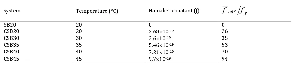
Hamaker constants, which are proportional to the magnitude of the IPF, were calculated from the results reported by Buoffard et al. [4]. The calcu-lated cohesive force was considered as the maxi-mum magnitude of van der Waals force. This maximum occurs when the surface distance be-tween particles or a particle and a wall, h, is the minimum separation distance of 0.4 nm. Hence, the Hamaker constant was calculated by consid-ering the van der Waals force to be equal to the cohesive force reported by Buoffard et al. [4] and the minimum separation distance. The Hamaker constants as well as relative cohesive forces (with respect to the weight of a particle) are given in Table 3 at various bed temperatures. In this table, the maximum van der Waals force is cohesive force used throughout this work.

4. Result and Discussion

4.1. Validation

In this study, the simulation results were validat-ed with experimental data of Shabanian and Chaouki [14, 15]. In their work, the instantaneous local bed voidage was measured by an optical fiber probe at various gas velocities in the bub-bling regime of fluidization. The fiber probe was positioned at the bed center at an axial position 20 cm above the distributor plate. The probability density distribution of instantaneous local bed voidage and the Eulerian solid velocity fieldwere compared with experimental data for validating the model.

4.1.1. Bed voidage distribution

The probability density distributions of the local bed voidage for SB20 and CSB30 at gas velocity of 0.9 m/s were taken from Shabanian et al. [14] .The simulated probability density distributions of the local bed voidage at Hamaker constants of 0 J (corresponding to SB20) and 3.6×10-19_J

(cor-responding to CSB30) at the superficial gas veloc-ity of 0.9 m/s were also obtained and compared with the experimental results in Fig. 2. This figure shows that there are two peaks in the local void-age distribution of both beds. The first peak at low voidage represents the emulsion phase and the second peak at high voidage is related to the bubble phase. It can be seen in Fig. 2 that there is a good agreement between simulated and exper-imental values.

4.1.2. Eulerian solid velocity field

For determining the Eulerian solid velocity field, bed width and bed height were divided into 20 and 80 equal parts, respectively, which resulted in having cells with size of 0.0025_{0.005 m. The}

particles were counted in each cell at each time step. Then, the summation of velocities of parti-cles in the same cell was divided by the number of particles in that cell to obtain the averaged parti-cle velocity. This averaging was done for the time span of 1 s.

9

the wall effect. The properties of bed,

particles and air are listed in Table 2. All the

simulations were continued for 15 s in real

time.

.

Table 3.

Calculated Hamaker constants at various bed temperatures

system

Temperature (



C)

Hamaker constant (J)

f

vdW

f

_g

SB20

20

0

0 CSB20

20

2.68 

10

-19

₂₆

CSB30

30

3.6 

10

-19

₃₅

CSB35

35

5.46 

10

-19

₅₃

CSB40

40

7.21 

10

-19

₇₀

CSB45

45

9.7 

10

-19

₉₄

Table 4.

Comparison of the dominant frequency for 3D and 2D beds using Equation (10)

Hamaker

constant (J)

Bubble

diameter (m)

Ratio of

frequencies

Bubble

frequency in

experiment

(Hz)

Bubble

frequency in

2D simulation

(Hz)

Bubble

frequency for

3D bubble

(Hz)

0

0.049

0.206

1.24

7.62

1.49

3.6 

10

-19

_0.0504

_0.207

_1.36

_7.8

_1.6

Hamaker constants, which are proportional

to the magnitude of the IPF, were calculated

from the results reported by Buoffard et al.

[4]. The calculated cohesive force was

considered as the maximum magnitude of

van der Waals force. This maximum occurs

(7)

Table 3. Calculated Hamaker constants at various bed temperatures

system Temperature (C) Hamaker constant (J)

f

uv

vdW

f

_g

SB20 20 0 0

CSB20 20 2.6810-19 ₂₆

CSB30 30 3.610-19 ₃₅

CSB35 35 5.4610-19 ₅₃

CSB40 40 7.2110-19 ₇₀

CSB45 45 9.710-19 94

Table 4. Comparison of the dominant frequency for 3D and 2D beds using Equation (10) Hamaker

con-stant (J) Bubble diameter (m) Ratio of frequen-cies Bubble frequency in experiment (Hz)

Bubble frequency in 2D simulation (Hz)

Bubble frequency for 3D bubble (Hz)

0 0.049 0.206 1.24 7.62 1.49

3.610-19 _0.0504 _0.207 _1.36 _7.8 _1.6

Hamaker constants, which are proportional to the magnitude of the IPF, were calculated from the results reported by Buoffard et al. [4]. The calcu-lated cohesive force was considered as the maxi-mum magnitude of van der Waals force. This maximum occurs when the surface distance

be-tween particles or a particle and a wall, h, is the

minimum separation distance of 0.4 nm. Hence, the Hamaker constant was calculated by consid-ering the van der Waals force to be equal to the cohesive force reported by Buoffard et al. [4] and the minimum separation distance. The Hamaker constants as well as relative cohesive forces (with respect to the weight of a particle) are given in Table 3 at various bed temperatures. In this table, the maximum van der Waals force is cohesive force used throughout this work.

4. Result and Discussion

4.1. Validation

In this study, the simulation results were validat-ed with experimental data of Shabanian and Chaouki [14, 15]. In their work, the instantaneous local bed voidage was measured by an optical fiber probe at various gas velocities in the bub-bling regime of fluidization. The fiber probe was positioned at the bed center at an axial position 20 cm above the distributor plate. The probability density distribution of instantaneous local bed

voidage and the Eulerian solid velocity fieldwere

compared with experimental data for validating the model.

4.1.1. Bed voidage distribution

The probability density distributions of the local bed voidage for SB20 and CSB30 at gas velocity of 0.9 m/s were taken from Shabanian et al. [14] .The simulated probability density distributions of the local bed voidage at Hamaker constants of

0 J (corresponding to SB20) and 3.6×10-19_J

(cor-responding to CSB30) at the superficial gas veloc-ity of 0.9 m/s were also obtained and compared with the experimental results in Fig. 2. This figure shows that there are two peaks in the local void-age distribution of both beds. The first peak at low voidage represents the emulsion phase and the second peak at high voidage is related to the bubble phase. It can be seen in Fig. 2 that there is a good agreement between simulated and exper-imental values.

4.1.2. Eulerian solid velocity field

For determining the Eulerian solid velocity field, bed width and bed height were divided into 20 and 80 equal parts, respectively, which resulted

in having cells with size of 0.0025_{0.005 m. The}

particles were counted in each cell at each time step. Then, the summation of velocities of parti-cles in the same cell was divided by the number of particles in that cell to obtain the averaged parti-cle velocity. This averaging was done for the time span of 1 s.

The experimental Eulerian solid velocity fields for SB20 and CSB40 at superficial gas velocities of 0.3 and 0.5 m/s by Shabanian and Chaouki [28] are presented in Fig. 3.

Figure 2. Comparison of simulated and experimental probability density distribution of local bed voidage at Ug

= 0.9 m/s (a) non-cohesive particles, (b) cohesive parti-cles [14]

This figure shows that there is a similar solid flow pattern in all cases, which is rising of particles to the splash zone through the central region of the bed and falling along the annulus. However, the solid flow pattern for CSB40 at 0.3 m/s diverged from the typical pattern, which is upward move-ment along the annulus in the bottom layer and identical to the typical solid flow pattern above the intermediate layer. In simulation, solid aver-age velocity was calculated for beds with

Hamak-er constants of 0 J and 7.2×10-19_{J at the}

superfi-cial gas velocities of 0.35 and 0.6 m/s and pre-sented in Fig. 4.

Figure 3. Effect of IPFs on the Eulerian velocity field of solids (a) SB20, Ug = 0.30 m/s, (b) CSB40, Ug = 0.30 m/s,

(c) SB20, Ug = 0.50 m/s, (d) CSB40, Ug = 0.50 m/s [28].

According to Fig. 4, the solid flow pattern for bed

with Hamaker constant of 7.2×10-19_{at 0.35 m/s}

(8)

100 S.M. Okhovat-Alavian et al. / Journal of Chemical and Petroleum Engineering, 52 (1), June 2018 / 93-105

harder for the gas to break down the particle-particle contacts rather than the particle-particle-wall contacts. Moreover, this figure depicts that creasing the superficial velocity results in in-creasing both the active height of the bed and the solid velocity. It can be further found from Fig. 4 that the particle average velocity decreases due to the presence of IPFs, which was reported by Wil-lett [36] too. By comparing Fig. 3 with Fig. 4 It can be found that the scale of vertical and horizontal axes of these two figures are not the same. In our simulation results, these scales are the same and we see the side view of the bed as a rectangle in the simulation and as a square in the experiment. By considering this point and comparing Fig. 3 and Fig. 4, it can be concluded that the model used in this work can predict the solid flow pat-tern in experiments correctly. Therefore, at all velocities considered in this study (bubbling re-gime), the 2D Cartesian simulation can be accept-ably predicted the results by the 3D cylindrical

experiment.

4.2. Distribution of bed voidage

To determine the effect of IPF on the distribution of gas between emulsion and bubble phases, sim-ulations were carried out with various values of Hamaker constant (i.e., various magnitudes of IPF). The probability density distribution of void-age at various Hamaker constants at the superfi-cial gas velocities of 0.9 m/s are shown in Fig. 5. As mentioned before, such a distribution contains two peaks for emulsion phase and bubbles. It can be seen in this figure that by increasing the IPF, the peak of emulsion phase shifts to higher val-ues. This means that the tendency of the fluidiz-ing gas passfluidiz-ing through the bed in the emulsion phase increases with increasing the IPF. In other words, by increasing the IPF in the bed, the emul-sion phase can hold more gas between particles. Similar trends were reported by other research-ers [26, 28, 39] concerning the effect of IPF on the emulsion voidage. This trend can be explained by the fact that existence of cohesive forces between particles leads to stickiness of particles which can hold a part of the particle weight. When particles collide, the particle-particle repulsion is less due the cohesive IPF which makes their movement to become limited. Therefore, particles cannot rear-range easily in the bed and particles cannot fill the cavities in their neighbors compared to the case when IPF is negligible. Consequently,

in-creasing the IPF results in formation of more cav-ities between particles in emulsion phase which is observed as greater emulsion voidage.

Figure 4. Effect of IPFs on the Eulerian velocity field of solids (a) H=0 J, Ug = 0.35 m/s, (b) H=3.610-19 J, Ug = 0.35

m/s, (c) H=0 J, Ug = 0.6 m/s, (d) H=3.610-19 J, Ug = 0.6

m/s

4.3. Bubble stability