Study of Magnetization Switching for MRAM Based Memory Technologies

(1)

University of New Orleans University of New Orleans

ScholarWorks@UNO

University of New Orleans Theses and

Dissertations Dissertations and Theses

12-20-2009

Study of Magnetization Switching for MRAM Based Memory

Technologies

Huy Pham

University of New Orleans

Follow this and additional works at: https://scholarworks.uno.edu/td

Recommended Citation Recommended Citation

Pham, Huy, "Study of Magnetization Switching for MRAM Based Memory Technologies" (2009). University of New Orleans Theses and Dissertations. 1028.

https://scholarworks.uno.edu/td/1028

This Dissertation is protected by copyright and/or related rights. It has been brought to you by ScholarWorks@UNO with permission from the rights-holder(s). You are free to use this Dissertation in any way that is permitted by the copyright and related rights legislation that applies to your use. For other uses you need to obtain permission from the rights-holder(s) directly, unless additional rights are indicated by a Creative Commons license in the record and/ or on the work itself.

(2)

Study of Magnetization Switching for MRAM

Based Memory Technologies

A Dissertation

Submitted to the Graduate Faculty of the University of New Orleans

in partial fulfillment of the requirements for the degree of

Doctor of Philosophy in

Engineering and Applied Science Physics

by

Huy Pham

B.S. Hanoi University of Science, Vietnam, 2001 M.S. University of New Orleans, USA, 2005

(3)

(4)

Acknowledgments

I am greatly thankful to my advisor, Prof. Leonard Spinu who taught me with a

wealth of knowledge in study and gave me a lot of helpful suggestions in life. This

dissertation could not have been done without his priceless guidance.

I would like to thank my supervisory committee members for their valuable and

insightful suggestions and guidance for this work and for various courses these last years

as well: Prof. Leonard Spinu, the committee chair, Prof. Leszek Malkinski, and Prof.

Ashok Puri from Department of Physics, Prof. Dimitrios Charalampidis from Department

of Engineering, and Prof. Scott L. Whittenburg, Vice Chancellor for Research and Dean

of the Graduate School at University of New Orleans.

I am deeply grateful to my colleagues: Dr. Dorin Cimpoesu, Dr. Ioan Dumitru, Dr.

Juliano Denardin, and Dr. Cosmin Radu for their support and valuable opinions. A lot of

results in this dissertation were contributed by their hard work.

I want to express my deepest gratitude for the continuous support from the

Advanced Materials Research Institute (AMRI) at University of New Orleans that offered

me a graduate research assistant position for all the duration of my studies. I also would

(5)

List of Figures

1.1. Considering an assembly of small magnetic particles ... 15

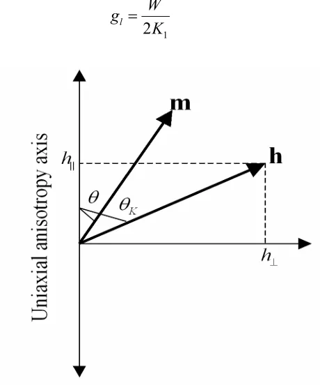
1.2. Relation between uniaxial anisotropy axis, m, and h... 16

1.3. Control plane of coordinates, and the astroid curve... 17

1.4. Graphical construction defining the possible m orientations... 18

1.5. Magnetization process and hysteresis loops... 19

1.6. Vector diagram for calculation of TS... 20

1.7. Illustrating the barrier energy and Néel-Brown model ... 24

1.8. Precessional motion of magnetization... 27

1.9. Magnetization torque with/without damping term... 30

1.10. Graphical representation of the LLG equation... 32

1.11. Magnetization vector m in spherical coordinates... 33

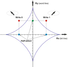
2.1. MRAM read operation ... 48

2.2. MRAM writing operation... 48

2.3. The critical curve and the operating regions in MRAM ... 50

2.4. Illustration of some complicated critical curves... 51

2.5. Vector diagram corresponding to a uniaxial anisotropy magnetic particle subjected to an external field... 54

2.6. The complex critical curves in eight regions... 56

2.7. Hysteresis loops in eight regions... 57

2.8. Transverse susceptibility curves in eight regions... 58

2.9. The behavior of magnetization in region III and V... 60

2.10. The astroid, hysteresis, and χ_T curves in region VI ... 61

2.11. The hysteresis, and χ_T curves in region VII... 62

2.12. The hysteresis, astroid, andχ_T curves in region VIII... 63

2.13. A thin film sample with coordinate system... 67

2.14. The theoretical curve determined from TS measurements... 68

2.15. TEM image of Co/SiO2 and schematic of TS experiment ... 69

2.16. Experimental critical curve for sample 90A... 70

2.17. Experimental critical curves for samples 90A, B, and 90C ... 72

3.1. Scheme of the magnetic field pulse... 76

3.2. Different representations of the precessional switching of an ellipsoidally shaped particle ... 77

(9)

3.4. Time evolution of magnetization vector in a field pulse 0.0/2.75/0.0 ns

of 50 Oe ... 79

3.5. Switching diagrams for different rectangular pulse lengths... 81

3.6. Switching diagram of the magnetization vector under a field pulse 0/0.25/0 ns ... 83

3.7. Time evolution of the magnetization components m_x, m_y, and m_z for the four parameter sets labeled (a)-(d) in Fig. 3.6... 83

3.8. Initial configurations of the system consisting of two ellipsoidal particles m₁ and m₂ ... 84

3.9. Switching diagram and phase portrait of an isolated ellipsoidal particle... 86

3.10. The phase portrait for the particle located at origin in interaction with a neighbor particle situated at the distance D=6 ... 88

3.11. Switching diagrams for two interacting particles with the separation between them D=6... 89

3.12. Switching diagrams for two interacting particles corresponding to the configuration of Fig 3.8(a) ... 91

3.13. Switching diagrams for two interacting particles corresponding to the configuration of Fig 3.8(b) ... 92

3.14. Switching diagrams for two interacting particles corresponding to the configuration of Fig 3.8(c) ... 93

3.15. Switching diagrams for two interacting particles corresponding to the configuration of Fig 3.8(d) ... 94

4.1. Illustration of the STT in a F/N/F pillar ... 98

4.2. Vector diagram of LLG’s equation with spin torque term added ... 104

4.3. Schematic of the free layer, assumed to be ellipsoid shaped ... 106

4.4. Time dependence of the applied current pulse... 107

4.5. AP-P switching diagrams at T =0 K, as a function of current pulse amplitude and duration at different values of damping constant α ... 110

4.6. AP-P switching diagrams at T =0 K for a current sweep rate 1 mA/ps I υ = , and α =0.01... 111

4.7. The precession of magnetization m under the influence of a spin current pulse at different values of the pulse duration ... 114

4.8. The precession of magnetization m under the influence of a spin current pulse at different values of the current sweep rate... 115

4.9. AP-P switching diagrams at T =0 K for a current sweep rate 0.05 mA/ps I υ = and υ_I =0.1 mA/ps... 116

4.10. AP-P switching diagrams at T =0 K for different initial orientation ϕ Δ of magnetization m ... 117

4.11. AP-P switching diagrams at T =0 K for different out-of-plane initial orientation Δθ of magnetization m... 118

(10)

4.13. Schematic of the free layer, assumed to be ellipsoid shaped, and single

domain, with an in-plane external applied field... 121

4.14. Switching diagrams as a function of the applied dc field for different values of the current pulse length... 122

4.15. Time switching as a function of the maximum value of a pulse field for different values of the current pulse length ... 125

4.16. Schematic of the pulsed field and current applied asyncronously ... 126

4.17. Time switching as a function of the maximum value of a pulse field with a current pulse applied at the delay time t₁ ... 126

5.1. Schematic representation of the SAF ... 130

5.2. Variation of the indirect exchange coupling constant... 131

5.3. Illustrative switching by SW reversal MRAM... 133

5.4. Illustrative switching by toggle MRAM ... 134

5.5. Schematic of the toggling operation of Savtchenko switching ... 134

5.6. Critical curves for different values of thickness ratio ... 138

5.7. Critical curves for different values of exchange coupling constant ... 139

5.8. Critical curves obtained by Fujiwara et al... 140

5.9. sCCs for a symmetric/asymmetric SAF ... 144

5.10. Switching diagrams of an asymmetric SAF at different values of υH... 146

5.11. Switching diagrams of an asymmetric SAF at different values of α ... 147

5.12. Switching diagrams of an asymmetric SAF at different values of T_H ... 148

5.13. Switching diagrams of a symmetric SAF at different values of υH ... 149

5.14. Switching diagrams of a symmetric SAF at different values of α ... 150

5.15. Switching diagrams of a symmetric SAF using B1 configuration ... 151

5.16. Switching diagrams of an asymmetric SAF taking into account both exchange and magnetostatic coupling... 152

5.17. Time dependence of the applied filed pulses ... 153

5.18. Toggle switching diagram of a symmetric SAF element at T =0 K for different values of the applied field sweep rate υ_H... 155

5.19. Toggle switching diagram of an asymmetric SAF element at T =0 K for different values of the applied field sweep rate υ_H ... 156

5.20. Toggle switching diagram of a symmetric/asymmetric SAF element at 0 K T = and time evolution of magnetization m... 158

5.21. Toggle switching diagram of a symmetric/asymmetric SAF element for different values of the damping constant α ... 159

5.22. Probability of switching of a symmetric SAF element for T =300 K ... 161

5.23. Probability of switching of an asymmetric SAF element for T =300 K ... 162

(11)

List of Tables

(12)

Abstract

Understanding magnetization reversal is very important in designing high density

and high data transfer rate recording media. This research has been motivated by interest

in developing new nonvolatile data storage solutions as magnetic random access

memories - MRAMs. This dissertation is intended to provide a theoretical analysis of

static and dynamic magnetization switching of magnetic systems within the framework of

critical curve (CC). Based on the time scale involved, a quasi-static or dynamic CC

approach is used.

The static magnetization switching can be elegantly described using the concept of

critical curves. The critical curves of simple uncoupled films used in MRAM are

discussed. We propose a new sensitive method for CC determination of 2D magnetic

systems. This method is validated experimentally by measuring experimental critical

curves of a series of Co/SiO2 multilayers systems.

The dynamics switching is studied using the Landau-Lifshitz-Gilbert (LLG)

equation of motion. The switching diagram so-called dynamic critical curve of

Stoner-like particles subject to short magnetic field pulses is presented, giving useful information

for optimizing field pulse parameters in order to make ultrafast and stable switching

(13)

For the first time, the dynamic critical curves (dCCs) for synthetic antiferromagnet

(SAF) structures are introduced in this work. Comparing with CC, which are currently

used for studying the switching in toggle MRAM, dCCs show the consistent switching

and bring more useful information on the speed of magnetization reversal. Based on

dCCs, better understanding of the switching diagram of toggle MRAM following toggle

writing scheme can be achieved.

The dynamic switching triggered by spin torque transfer in spin-torque MRAM

cell has been also derived in this dissertation. We have studied the magnetization’s

dynamics properties as a function of applied current pulse amplitude, shape, and also as a

function of the Gilbert damping constant. The great important result has been obtained is

that, the boundary between switching/non-switching regions is not smooth but having a

seashell spiral fringes.

The influence of thermal fluctuation on the switching behavior is also discussed in

this work.

Keywords: magnetization switching, critical curve, SAF, MRAM, toggle MRAM,

(14)

Introduction

Magnetization dynamics is one of the central issues in the physics of mesoscopic

magnetic systems [1, 2] and its understanding is important not only for its evident

fundamental interest but also due to the big impact on the information technology, more

specifically on magnetic information storage. Magnetic recording is rapidly approaching

the nanometer scale as storage densities are projected to increase to a terabit per square

inch. High volume of data requires higher data transfer rates. These present new

challenges and opportunities in nanometer scale materials engineering and in

inderstanding the magnetic properties of nanometer scale magnetic materials. Among the

critical issues is the manner and speed which the magnetization direction can be reversed

from one stable configuration to another. Also, for the magnetic random access memories

(MRAMs) [3] unlike present forms of nonvolatile memories, they must have switching

rates and rewrite-ability properties surpassing those of conventional RAMS. This can be

achieved only first by understanding and then by controlling the magnetization dynamics

of very confined magnetic elements.

The magnetization dynamics at different timescales is governed by different

physical dynamic mechanisms. Firstly, on the nanosecond range (0.1 ns to 100 ns) the

dipolar interactions, external fields and spin–lattice interactions are the major driving

(15)

which is the primary source of magnetization rotation that is gradually opposed by

damping [4, 5]. This regime is described theoretically by the phenomenological

magnetization’s equation of motion Landau-Lifshitz-Gilbert (LLG) and is able to

describe the precessional reversal mechanism. In this regime, the weakly damped

precession of spins induces the so-called ringing of magnetization, which can persist up

to several nanoseconds. Recently, it was shown that it is possible to suppress the ringing,

and so reduce the switching time through a ballistic switching process, by matching the

field-pulse parameters to the frequency and the phase of the magnetic excitation [4]. For

shorter time scales of the order of picoseconds (1-100 ps) the electron excitations cannot

be ignored and electron-phonon, phonon-phonon, and spin-lattice interactions start to be

important. In this case the LLG formalism gradually becomes invalid as quantum effects

appear. Here a new mechanism of magnetization reversal is possible, induced by an

angular momentum transfer from a magnetically polarized electron current [6-9]. Finally,

for very short time scales (1fs-1ps), electron–electron and spin-orbit interactions

dominate. Magnetic structures can be excited by optical probes that are shorter than

fundamental timescales such as spin-lattice relation times and precession times. This

regime became accessible only recently when novel pulsed magneto-optical lasers were

developed capable of studying the spin dynamics at femtosecond resolution [10, 11].

This thesis is intended to provide a theoretical analysis of magnetization dynamics

in nanometer scale magnetic structures in the first regime among those mentioned above.

In spite of continuous efforts on studying this dynamics, there are several fundamental

(16)

interactions, the spin-torque transfer effects, the role of thermal fluctuations, and the

basic mechanism of damping of magnetization motion. Specifically, in this work the

study of magnetization dynamics will be performed using the formalism of the critical

curve. The critical curve is a very important concept for both, theoretical study of

switching mechanism in magnetic system and device applications, as MRAM. The

critical curve was first discussed by Slonczewski [12] and then developed further by

André Thiaville in 1997 [13]. However, the name of “critical curve” basically comes

from the Stoner-Wohlfarth model, which was early introduced by Stoner and Wohlfarth

to describe the simplest case of the uniaxial, single domain particles in 1947 [14]. Based

on the remarkable properties of the critical curve, the hysteresis and the corresponding

transverse susceptibility curves can be constructed, providing a lot of useful information

of magnetic materials. It is clear, therefore, that the critical curve is the key to the

understanding of the static behavior of magnetic materials. There are several techniques

developed so far to measure the critical curve. In the first part of this work the

quasi-static case will be considered where a new method for measuring the quasi-static critical curve

using the reversible susceptibility measurements is proposed. This method will be

theoretically presented and experimentally validated in the case of a nanostructured

magnetic system consisting of multilayers of Co/SiO2.

In the case of faster magnetization switching, a dynamic critical curve approach is

used. The switching properties are discussed in the case of interacting single domain

particles subject to an external field pulse. The theoretical description of precessional

(17)

equation that includes the pulse magnetic excitation, the exchange and dipolar interaction

fields. The weakly damped precessions of spin induce small fluctuation of magnetization,

or in other words, ringing of magnetization, for a time of nanoseconds. The ringing of

magnetization is strongly dependent on field pulse parameters (as shape, rising and

falling times) and a precise control of ultra fast magnetization can be obtained. The main

goal is to determine the parameters of field pulse for which a fast and stable switching

can be achieved. The influences of interaction between particles and the spatial

placement of the particles on switching behavior are discussed. Our results and analysis

suggest that in dealing with the problem of improving the density of data storage in

MRAM, the dipolar interaction between neighboring magnetic elements is one of

important aspects that needs to be considered carefully.

Recently, there are several novel approaches that eliminate the half-select disturb

phenomenon present in conventional MRAM [15-18]. Among them, “magnetization

toggling” and “spin torque transfer” switching are the most promising, introducing new

advanced generations of MRAM, as “toggle-MRAM” and “Spin transfer torque

MRAM”, respectively. This study is also motivated by the considerable interest in

investigating the dynamic switching properties of magnetization in these new advanced

types of MRAM. In toggle MRAM, proposed by Savtchenko [15], the free layer in a

MRAM cell consists of two weakly anti-parallel coupled ferromagnetic layers instead of

a single layer as used in conventional MRAM. Therefore, the free layer in a toggle cell is

a synthetic antiferromagnet (SAF) trilayer stack. The theory of simple uncoupled films of

(18)

approach was developed [19-21]. Subsequently, CCs of SAF have been extensively

studied due their technological important for toggle-MRAM [22-29]. However, the CCs

of SAF are restricted only to a quasistatic regime, where the magnetization dynamics and

precessional effects are neglected. As demanding for a high throughput and very short

access time, the magnetization is forced by pulsed magnetic fields to switch at

nanosecond and sub-nanosecond time scales for which the static CC approach is not

anymore adequate. In this dissertation, a dynamic generalization of critical curves for

coupled thin films is presented, analyzing the magnetization switching of SAF elements

subjected to pulsed magnetic fields. The boundary between switching/non-switching

regions represents the natural generalization of static CC, namely the dynamic CC (dCC).

Our original contribution to the study of dCCs gives better understanding of the toggle

dynamic switching mechanism in Toggle MRAM.

The other advanced generalization of MRAM based on “spin transfer torque”

switching approach, so-called spin transfer torque MRAM (STT-MRAM), also attracted

an increased interest [16-18]. The concept of spin angular momentum transfer torque was

proposed in 1996 by Slonczewski [8] and Berger [6]. In the presence of an electric

current, a torque may act on the magnetization of a thin ferromagnetic layer, arising

primarily from the transmission and reflection of incoming electrons. The spin-torque

offers a new way to control the writing process in high density MRAM because a

spin-polarized current can switch the magnetization of a ferromagnetic layer more efficiently

than a current-induced magnetic field. An essential problem in the development of a

(19)

current that ensures a reliable magnetization reversal at high operating frequencies. In

this work we present how the current sweep rate, damping constant, initial position,

waiting time, and also thermal fluctuation affect the switching, the reliability, and the

writing speed of spin-torque devices. The main goal is to determine the optimum

parameters of current pulse to achieve a fast and stable switching.

In this thesis, these two recent developments of MRAM mentioned above will be

studied by comprehensive micromagnetic simulations. To be more specific, we shall now

outline the organization of the dissertation below:

Chapter 1, Overview of Magnetism, gives an overview of the background

information required for a full understanding of the remainder of the thesis. The

background information includes a short presentation of the free energy of magnetic

systems, Stoner-Wohlfarth and Néel-Brown models and LLG/stochastic equations of

motion.

Chapter 2, Static Critical Curve, begins with a brief description of the importance

of the critical curve in magnetization switching processes in general and in MRAM

technology in particular. Based on the remarkable properties of the critical curve, the

hysteresis and the corresponding transverse susceptibility curves are also determined and

discussed. The final point of this chapter is concerned about our new sensitive method

based on susceptibility measurements for the critical curve determination of

two-dimension (2D) magnetic systems.

Chapter 3, Magnetization Dynamics in Interacting Magnetic Systems, presents the

(20)

pulses, obtained by numerical investigations of the Landau-Lifshitz-Gilbert equation. The

switching properties are discussed as a function of the external field pulse strength and

direction, pulse length and the pulse shape. We advanced the work of M. Bauer and his

co-authors [4] that was developed for non-interacting systems, and we have studied the

dynamic magnetization behavior of a MRAM cell taking into account the dipolar

interaction with neighboring cells.

Chapter 4, Spin Transfer Switching, presents our original contribution to the

problem of dynamic magnetization switching triggered by spin angular momentum

transfer in a pulsed current of a spin-valve-type trilayer structure, and its dependence on

thermal effects. The magnetization switching under coexistence of the spin-transfer

torque and the torque by a pulsed magnetic field is also discussed in this chapter. Our

model is based on the LLG equation and the stochastic LLG equation with a spin-transfer

torque term included.

Chapter 5, Static and Dynamic Critical Curves of a Synthetic Antiferromagnet,

begins with a brief description of a synthetic antiferromagnet (SAF) and its technological

applications. The static critical curve of SAF and its remarkable properties in

understanding the magnetization switching mechanism in Toggle-MRAM are presented.

Then, we discuss our original contribution to the study of a dynamic generalization of

critical curves for SAF structures, analyzing the magnetization switching of SAF

elements subject to pulsed magnetic fields. In order to determine dynamic critical curves

(dCCs) dependence on field pulse’s parameters, we have studied the switching properties

(21)

the dCCs, we further investigate the dynamic toggle switching in toggle MRAM and its

dependence on thermal effects.

Finally, conclusions are drawn in the last chapter.

Each of the last four chapters ends with a summary that briefly presents the

essential information such way that one can faster focus its attention on a specific section.

The dissertation ends with a list of author’s publications and a short Vita. The list

of publications includes also several papers published during the last year pertinent to an

experimental work that the author carried out in the framework of a collaborative work

between Prof. Spinu’s research group and Prof. Zhiqiang Mao’s group from Tulane

Universitiy. This works is not directly related to the theoretical work presented in this

thesis and is concerned with the study of the newly discovered family of unconventional

(22)

Chapter 1 Overview of Magnetism

Magnetism is certainly one of the cornerstones of what we today call the

information technology era. Following the huge development of electronic devices such

as the personal computer, this era has been strongly driven by the growing demand to

increase the density and the speed of writing and retrieving data in memory devices.

Today, the demand for information storage is enormous and expected to increase even

further. High density of data requires higher data transfer rates. These present new

challenges in understanding of the magnetization behavior from both static and dynamic

points of views. The understanding of the magnetization reversal is extremely important

not only for its evident fundamental interest but also due to the big impact on the

information technology.

This chapter will present the most important contributions to the free magnetic

energy, and the overview of some basic theoretical models describing the static and

dynamic behavior of magnetization. The Stoner-Wohlfarth model regarding the static

switching behavior of an assembly of single domain ferromagnetic particles, the

Néel-Brown model for the system of superparamagnetic particles, as well as the LLG equation

(23)

1.1 Magnetic free energy

The following section is intended to facilitate the understanding of the concept of

the energy of magnetic systems. As we all know the problem of investigating the static

equilibrium of a system is always related to the problem of minimizing the total free

energy of the system. For instance, in Stoner- Wohlfarth model (SW) [14] by finding the

total magnetic energy minima, it is possible to predict the magnetization rotation and

switching behavior of the particle under the influence of an applied field. Another

straightforward example is that the existence of well-known domain structure in

ferromagnetic materials can be explained by the result of minimization of the total free

energy. In general, in order to observe the behavior of a magnetic system, it is of

important to fully understand the contribution of each energy term in the total free energy

of the system. In the following, we shall present the most important energy terms.

1.1.1 Magnetocrystalline anisotropy

In a magnetic crystal, the disposition of the magnetic moments reflects the

symmetry of the lattice. Interactions of the magnetic moments between themselves or

with the lattice are thus affected by the symmetry of the crystal and give rise to

anisotropic energy contributions, summarized under the term of magnetocrystalline

anisotropy [30]. Therefore, there are directions in space lattice along which it is easier to

magnetize a given crystal than in other directions. These directions are called easy

directions. Let us now consider the simplest case of the uniaxial magnetic anisotropy,

and suppose that the uniaxial anisotropy axis, or easy axis, is parallel to the c-axis of the

(24)

axis, and depends only on the relative orientation of magnetization vector M with respect

to the axis. As M rotates away from c-axis, the anisotropy energy initially increases with

θ, the angle between the c-axis and the magnetization vector, then reaches a maximum

value at _θ ₌₉₀0_{, and decreases to its original value at}_θ ₌₁₈₀0_{. In other words, the}

minimum of anisotropy energy occurs when the magnetization points in either the + or –

direction along the c-axis. We can express this energy density as follows:

2 4

0 1sin 2sin ...

K

W =K +K θ +K θ+ (1.1)

The coefficients K_n

(

n=0, 1, 2....

)

are called anisotropy constants, having the dimension of energy per unit volume. The higher-order terms above K₂ are negligible since they are

very small. The K0 term is a constant; therefore, it also can be disregarded. For small

deviations of the magnetization vector from the equilibrium position, the anisotropy

density can be approximated, to second order in θ, as

2

1 2 1 2 1cos 2 1 .

K K

W ≅Kθ ≅ K − K θ = K −M H (1.2)

Where 2 1

K s K H

M

= , with M_s is the magnitude of the magnetization vector M. H_K is called

the anisotropy field, giving a natural measure of the strength of the anisotropy effect and

of the torque necessary to take the magnetization away from the easy axis. For cubic

crystals, the anisotropy energy can be expressed in terms of the direction cosines

(

α α α1, , 2 3

)

of the magnetization vector with respect to the three cube edges

2 2 2 2 2 2 2 2 2

1( 1 2 2 3 3 1) 2 1 2 3

K

(25)

1.1.2 Magnetostriction and stress anisotropy

Magnetostriction is the phenomenon whereby the shape and volume of a magnetic

specimen change during the process of magnetization. The reason for this behavior is that

the crystal lattice inside each domain is spontaneously deformed in the direction of

domain magnetization and its strain axis rotates with the rotation of the domain

magnetization, thus resulting in a deformation of the specimen as a whole [30]. The

magnetoelastic energy density for isotropic magnetostriction is given by:

2

3

sin

2 s s

W_σ = λ σ θ (1.4)

where θs is the angle between the magnetization and the stress direction, λs is the

appropriate magnetostriction constant, σ is a uniaxial stress applied along the certain

direction.

1.1.3 Shape anisotropy

The origin of shape anisotropy is magnetostatic energy. The magnetization curve

of a material depends not only on its magnetic susceptibility, but also on the shape of the

specimen. When a specimen of finite size is magnetized by an external magnetic field,

the free poles, which appear on its ends, will produce a magnetic field directed opposite

to the magnetization [30]. This field is called the demagnetizing field, and is given by:

d = −N

H M (1.5)

where N is called the demagnetizing factor, which depends only on the shape of the

specimen. For a single domain particle, the magnetostatic energy is related to the

(26)

ellipsoidal shape. If we take the principal axes a, b, and c of the ellipsoid as Cartesian

axes, the magnetostatic energy density takes the form

1₍ 2 2 2₎

2

D a x b y c z

W = N M +N M +N M (1.6)

where N_a, N_b and N_c are the demagnetizing factors pertaining to the three principal

axes, and satisfy the equation N_a +N_b+N_c =4π (in cgs units system).

It is well known that the longer the principal axis, the lower the corresponding

demagnetizing factor and the lower the energy when M points along that direction.

1.1.4 Zeeman energy

Zeeman energy is simply the energy of the interaction between the magnetization

vector and the external applied field, given as:

WH = −M H. (1.7)

1.1.5 Exchange energy

The exchange interaction was first introduced by Heisenberg in 1928 to interpret

the origin of the enormously large molecular fields acting in ferromagnetic materials.

This interaction is due to a quantum mechanical effect. The energy of exchange

interaction is given by: _E 2 _ij

ij

W = −

∑

J S S_i _j (1.8)

where S_i, S_j are spins. The term J_ij, which has no corresponding concept in classical

physics, is called the exchange integral. Here J_ij >0 brings two spins parallel to each

other (ferromagnetism) whereas J_ij <0 brings two spins anti-parallel to each other

(27)

1.2 Stoner-Wohlfarth model

Based on the understanding of energy terms defined previously, we are able to

study the magnetization process of magnetic systems through various models. It is well

known that a magnetic body, in general consists of many domains, or in other words has

a multi-domain structure. Thus, the magnetic system is divided into uniformly

magnetized regions (domains) separated by domain walls in order to minimize its total

free energy. However, due to the energy cost of the domain walls formation, the balance

with the magnetostatic energy limits the subdivision in domains to a certain optimum

domain size. As a matter of fact, there is a corresponding lower limit in the crystal size,

below which a single-domain structure does exist, since the energy increase due to the

formation of domain walls in this case is higher than the energy decrease obtained by

dividing the single domain into smaller domains [31].

The magnetization behavior of an assembly of single domain ferromagnetic

particles has been one of the central issues in the physics of magnetism. Many different

models have been taken, in which, Stonne-Wohlfarth (SW) model is one of the simplest

and successful approaches. In 1948, starting from the assumption that it is possible to

identify all magnetic particles which reverse their magnetization by coherent rotation,

Stoner and Wohlfarth came up with a model to describe such a system [14]. The basic

idea of their model, or coherent rotation model, is that a single magnetization vector is

sufficient to describe the state of the whole system. This reduces the number of degree of

freedom to one. The approach is somehow idealized and should not be expected to give

(28)

monodomain particle in which the exchange interaction will be able to keep the

elementary spins parallel with respect to each other so that the whole system can be

considered uniform as a big single magnetization vector (see Fig. 1.1). One additional

notable exception of SW model is that the temperature of the system is not taken into

account or, in other words, it can be considered equal to zero. This can be reasonable

when the sizes of all ferromagnetic particles are still large enough so that the thermal

energy is negligibly small, compared to the anisotropy energy E KV= . In this case the

magnetic relaxation (superparamagnetism) phenomena can be disregarded. Also, the SW

model does not take into account the interaction between particles.

Figure 1.1. Considering an assembly of small magnetic particles as a big single moment.

1.2.1 The free energy function

Let us now firstly consider the free energy of a single-domain SW particle. The

free energy of the uniaxial particle per unit volume is composed of two terms, the

magnetocrystalline anisotropy energy and the energy of interaction with the external

(29)

(

)

2 1

, sin _s cos( _K)

W θ H =K θ−M H θ θ− (1.9)

where K₁ is the first anisotropy constant, H the external field, θ and θ_K the angles made

by normalized vectors

S M

= M

m and

K H

= H

h (see Fig. 1.2). It would be convenient to

write (1.9) in dimensionless form, by introducing the dimensionless quantity:

1 2 l W g K

= (1.10)

Figure 1.2. Relation between uniaxial anisotropy axis, magnetization unit vector m, and external field, h.

With this notation (1.9) becomes:

( )

_, 1_sin2 _cos

(

)

2

l K

g θ h = θ −h θ θ− (1.11)

Instead of using the variables ( ,hθ_K) in (1.11) one can use the field components

perpendicular and parallel to the easy axis (h_⊥ =hsinθ_K ; h_|| =hcosθ_K) obtaining:

2

||

1

( , ) sin sin cos

2 l

(30)

1.2.2 Astroid curve

Now we would be able to observe the change of the energy function when we

move around in the control plane represented by the plane of coordinates h_⊥andh_||. By

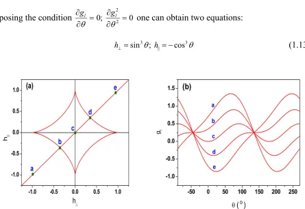
taking the first and second derivative of the energy function as described in (1.12) and by

imposing the condition 0; ₂ 0

2

= ∂ ∂ = ∂ ∂

θ

θl l

g g

one can obtain two equations:

3 3

||

sin ; cos

h_⊥ = θ h = − θ (1.13)

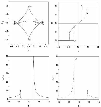
Figure 1.3. (a) Control plane of coordinates h and h_⊥. The astroid curve defined by (1.13). (b) Examples of the dependence of the system energy g_l in (1.12) on θ at different points in control space are shown.

The curve generated by (1.13) when θ varies in the interval

(

0, 2π

)

as shown in Fig. 1.3(a) is the critical curve or astroid curve [32]. The figure 1.3(b) shows the energy

obtained from (1.12) as a function of θ at different values of the applied field

(31)

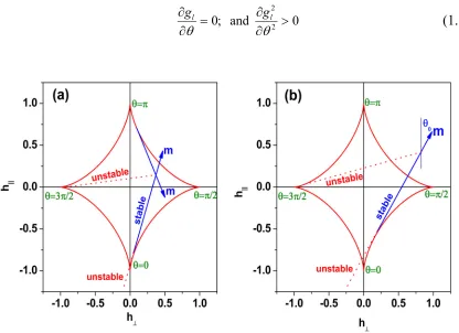
The astroid curve has remarkable properties. The orientations of m for a given

field h can be determined by drawing the tangents to the astroid passing through the

point h of the control plane (see Fig. 1.4). Each tangent may identify either a stable or an

unstable state. The stable orientation provides an energy minimum, and it can be selected

using the two conditions:

0; and ₂ 0

2

> ∂ ∂ =

∂ ∂

θ

θl l

g g

(1.14)

Figure 1.4. Graphical construction defining the possible m orientations associated with a given applied field: (a) Inside the astroid. (b) Outside the astroid. The straight half-lines marked as “stable” (“unstable”) are sets of local energy minima (maxima) characterized by the same m orientation. θ values show how the angle parameter of (1.13) varies along the astroid.

As a result, we can easily realize that there is only one stable solution when the

point is located outside the astroid, whereas there are two stable tangents that can be

(32)

Figure 1.5. (a) Magnetization process under alternating field. Black arrows represent the m orientation in the state occupied by the system, white arrows in the other state available to the system. (b) Hysteresis loops for different values of θ_K.

1.2.3 Hysteresis

The typical properties of the astroid curve discussed above are the basis for the

analysis of the phenomena taking place when the field is slowly varied over time. The

magnetization process under alternating field, where h oscillates between opposite

values along a fixed direction, is shown in Fig. 1.5(a). The field representative point

moves back and forth in control space along a fixed straight line. The m orientation at

each point is obtained by the tangent construction discussed in the preceding subsection.

Inside the astroid, two orientations are possible, and the one actually realized depends on

the past history. If the field oscillation were all contained inside the astroid, the

magnetization would reversibly oscillate around the orientation initially occupied. If the

field can cross over the astroid boundary, a magnetization reversal (Barkhausen jump)

(33)

1.2.4 Reversible transverse susceptibility

In the previous section we showed the importance of the astroid, or in general of

the switching critical curve. There are several methods [33, 34] for determining

experimentally the critical curve of magnetic materials and the reversible transverse

susceptibility (RTS) is one of them [35]. In the next chapter we will discuss this method

in some detail and the crucial role of RTS in studying the magnetization process.

Therefore, it is worth mentioning here how to obtain the RTS based on the SW model.

Figure 1.6. The vector diagram corresponding to a uniaxial magnetic particle subjected to a magnetization process in perpendicular fields.

The reversible transverse susceptibility (RTS),χ_T, is actually a component of the

reversible susceptibility (RS) tensor [36]. In order to define this tensor; one considers a

magnetic field H applied along to z-direction of a ferromagnetic specimen. For a change

ΔH of the field, the RS tensor, χik, is defined as ΔMi =χikΔHk, for ΔHk →0, provided

(34)

results that one has two components for RTS measured in two perpendicular directions

with respect to the applied field, and given by:

1

0

, 0

z x T y x H dM _H dH χ = ⎛ ⎞ =_⎜ _⎟ =

⎝ ⎠ (1.15)

2

0

, 0

y y T x y _H dM H dH χ = ⎛ ⎞ =_⎜ _⎟ =

⎝ ⎠ (1.16)

We will briefly outline the derivation of theχ_T expression in the case of a uniaxial

single-domain SW particle with the first anisotropy constant K₁, and the saturation

magnetization MS. Based on the spherical coordinate system as shown in Fig. 1.6, the free

energy density of the magnetic system, W W= _K +W_H, considered in the dimensionless

form of h HM= _S / 2K₁ is

(

)

2

1

sin cos sin cos sin sin sin sin cos cos

2 (sin sin cos cos cos )

K K M M K K M M K M

H M M H M

W K

hK

θ ϕ θ θ θ ϕ θ θ θ θ

θ θ ϕ θ θ

= − + +

− + (1.17)

The angle θ_M and ϕ_M will be determined from two conditions of minimizing the free

energy 0, and 0

M M

W W

θ ϕ

⎛ ∂ ₌ ∂ ₌ ⎞

⎜_∂ _∂ ⎟

⎝ ⎠ as follows:

(

)

(

)

2 2

2

sin sin 2 cos ( ) sin 2 cos 2 cos

cos sin 2 2 cos sin sin cos cos 0

K M K M K M K M

K M h H H H M M

θ θ ϕ ϕ θ θ ϕ ϕ

θ θ θ θ θ θ ϕ

− + −

− − − = (1.18)

(

)

(

)

sin sin sin sin

sin sin cos cos cos sin sin 0

M M K K M

K M K M K M h M M

θ θ θ ϕ ϕ

θ θ ϕ ϕ θ θ θ ϕ

−

⎡ − + ⎤− =

⎣ ⎦ (1.19)

In the limit θ_H →0, the equation (1.19) can be rewritten as

M K n

(35)

where n is an integer. In most cases n=0, but there are some cases in which n=1 give the energy minimum. In the limit θ_H →0, and using either of the condition n=0 or

1

n= , the equation (1.18) reduces to:

sin 2

(

θ_M −θ_K

)

+2 sinh θ_M =0 (1.21)

or sin 2

(

θ_M +θ_K

)

+2 sinh θ_M =0 (1.22)

From the figure 1.6, we have:

H_x =Hsinθ_H, cosH_z =H θ_H, sinM_x =M_s θ_M cosϕ_M

Hence,

(

)

(

)

0 0

sin cos 3

2 H sin

M M T H d Lim d h θ θ ϕ χ

χ = → θ (1.23)

where 2

0 Ms / 3K1

χ = . By differentiating (1.18) and (1.19) with respect to θ_H, and using

(1.20) in the case of n=0 one can obtain the final expression for χT as follows

2 2

₍

₎

2

(

)

0

sin cos

3

cos sin

2 cos cos 2 sin

K M

T M

K K

M M K K

h h θ θ χ _ϕ θ _ϕ χ θ θ θ θ ⎡ − ⎤ = _⎢ + _⎥ + − ⎢ ⎥

⎣ ⎦ (1.24)

This expression of TS of SW particles in (1.24) was first obtained by Aharoni [36]. A

complete analysis of TS curve in the case of quartic crystalline anisotropy will be given

in the next chapter.

1.3 Néel and Brown models

When the system of small single domain particles is concerned, the thermal effect

needs to be taken into account since in this case the thermal energy of the system is

comparable to the magnetic anisotropy energy barrier of single domain particles.

(36)

particle is given by _{E KV}₌ _sin2_θ _where_K_{is the anisotropy constant and}_θ_{the angle}

between the magnetization vector and the easy axis. Thus, the energy barrier, separating

easy directions is E_B =KV , proportional to the volume V . Therefore by decreasing

particle size the anisotropy energy decreases, and for a size lower than a certain value, it

may become comparable to or even lower than the thermal energy kT. This implies that,

the energy barrier for magnetization reversal may be overcome, and then the magnetic

moment of the particle can thermally fluctuate from one easy direction to the other, even

in the absence of the applied field, like a single spin in a paramagnetic material. The

magnetic behavior of an assembly of such small particles is called superparamagnetism

[31]. In the case of dealing with a system of magnetic nanoparticles concerning the

occurrence of superparamagnetism, the SW model failed to describe such a system. The

thermal fluctuation of the magnetic moments of a single-domain particle and its decay

toward thermal equilibrium was then introduced by Néel [37] and further developed by

Brown [38]. The main difference between these two authors is the pre-exponential factor

in their formulas. This pre-factor depends on several parameters such as damping,

temperature and exchange interaction. For simplicity, the pre-factor is assumed to be

constant, and this assumption became well known as the Néel-Brown model. This model

is widely used in magnetism, particular in order to describe the temperature and

time-dependence of the magnetization. However, in this work it will not be discussed in detail

but briefly. The model stated that the timescale for magnetization reversal τ , in a single

particle with uniaxial anisotropy, depends on the anisotropy energy barrier ΔE and the

(37)

) / exp(

0 ΔE kT

=τ

τ (1.25)

The pre-exponential factor τ₀ as mentioned above depends on various parameters

but typically is in the timescale ₁₀−9_s_{and plays a crucial role in determining the resulting}

time frame for superparamagnetic relaxation and hence the blocking behavior observed

by a particular technique.

Figure 1.7. Illustrating the barrier energy and Néel-Brown model.

From (1.25), one can see that for the fine magnetic particles the actual magnetic

behavior depends on the measuring time τ_m of the specific experimental technique with

respect to the relaxation time τ associated with the overcoming of the energy barriers. If

m

τ >τ , the relaxation appears to be so fast that the magnetic moment can easily overcome

the energy barriers and the assembly of particles behaves like a paramagnetic system

(38)

the energy barrier is negligible, the relaxation appears so slow that the assembly of

particles will be in blocked state (ferromagnetic state) (see Fig. 1.7).

The blocking temperature TB, separating the two states, is defined as the

temperature at which measuring time becomes equal to relaxation time, i.e.

τ_m =τ =τ₀exp(ΔE/kT) (1. 26)

Therefore the blocking temperature is not uniquely defined but it related to the time scale

of the experimental technique.

In this work, we only investigate theoretically the magnetization dynamics under

thermal relaxation. Thus, the magnetization dynamics we will mainly focus on is related

with the time necessary for a system to reverse the magnetization. This aspect could not

be achieved in the framework of SW model, but only by using a time dependent equation

of motion of magnetization. This will be the object of the following sections.

1.4 Landau – Lifshitz – Gilbert equation of motion

The behavior of the magnetization of a single domain ferromagnetic particle has

been the subject of many studies. As mentioned in the preceding section, the SW model

can describe the system of single domain particles, provided that the coherent rotation

condition is satisfied, and the magnetic relaxation (superparamagnetism) phenomena and

the interparticle interactions can be neglected. The SW model, however, says nothing

about two other important aspects: how the system will approach equilibrium and how

the magnetization will react to a time-varying applied field. In order to discuss these

(39)

magnetization in a homogeneously magnetized body. This equation is useful not only to

describe the equilibrium position but also the dynamics of the moment reaching that

position. Gilbert then modified it in 1955 to overcome the unphysical solution for large

damping parameters [40]. Because the so-called Landau – Lifshitz – Gilbert (LLG) is a

nonlinear differential equation, analytical solutions can be found only in special cases.

1.4.1 The gyromagnetic equation

Let us firstly consider the LLG equation in the absence of the damping term. It is

well known that the magnetic moment of an electron is related to spin momentum by:

M=γS (1.27)

where γ is the gyromagnetic ratio for an electron spin, given by

2 ge mc

γ = − (1.28)

Here, e is the electron charge, m the electron mass, c the velocity of light, and g the

Landé splitting factor. It is worth pointing out that since the charge of an electron is

negative, γ is a positive constant. However, Landau and Lifshitz used a negative γ and

consequently so did many researchers [41].

The equation (1.27) is valid in both classical and quantum mechanics. The torque

exerted on a magnetic moment M by a magnetic field H is

T M H= × (1.29)

Equations (1.27) and (1.29) give an equation of motion for the magnetic moment

(40)

d

dt =γ ×

M

M H (1.30)

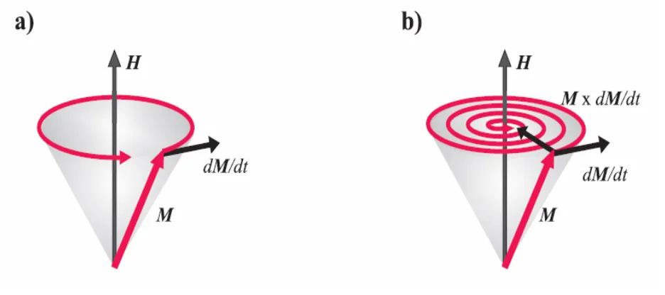
The simple gyromagnetic equation (1.30), simply describes an instantaneous precessional

motion of the magnetization vector, as sketched in Fig. 1.8. This is the most basic

equation describing the dynamic behavior of the magnetization of a single domain

ferromagnetic particle.

Figure 1.8.Precessional motion of magnetization.

The applicability of (1.30) is not limited to the torque exerted by an external magnetic

field. Any torque on a magnetic moment M can be written in the form of (1.30) if we

define an “effective” magnetic field:

( ) E ∂ = −

∂

M H

M (1.31)

where E( )M is the potential energy of the system with respect to the work done by

(41)

studies of the properties of ferromagnets have led to identification of five different

domain energy terms

(

H D E K

)

E= W +W +W +W +W_σ ∗V (1.32)

where V is the volume and W_H is the external field energy density, W_D is the

demagnetization energy density, W_E is the exchange energy density, W_K is the anisotropy

energy density, and W_σ is the magnetoelastic energy density. The corresponding effective

fields are

Total = H + D+ E + K + σ

H H H H H H (1.33)

The first two terms are magnetic fields. The last three are effective fields that have

quantum mechanical origins.

1.4.2 The Landau-Lifshitz equation

The equation (1.30) represents uniform undamped precession of the vector M

about the axis of the field H. The observable behavior, however, of the magnetization of

a single domain ferromagnetic particle, is that of alignment of M with H in time. This

alignment is due to the collisions between precessing electrons which take place within

particle. It is apparent, therefore, that the field does not directly cause alignment; rather it

causes a precession of M about the axis of the field, which along with collision will

produce alignment. With the aim of including this fact in the mathematical analysis,

Landau and Lifshitz introduced a second term into the gyromagnetic equation (1.30), the

tendency of which is to align M with H. In their 1935 paper [39], they proposed an

(42)

(M H× )×M H M M= ( . ) ( . )− H M M (1.34)

The Landau-Lifshitz equation in the original form is:

(

)

2 . s M γ ⎡ λ⎛ ⎞⎤ = − _⎢ × + _⎜ − _⎟_⎥ ⎢ ⎝ ⎠⎥ ⎣ ⎦

H M M

M H M H (1.35)

where λ is a constant of the same dimensions as M_s and limited by the condition that

s M

λ . Using (1.34), the Landau-Lifshitz equation is more commonly written in the

following form: ₂

s M

γλ γ

= × − × ×

M M H M H M (1.36)

This equation now represents damped precessional motion, wherein alignment ultimately

takes place between the two vectors, M and H.

1.4.3 Gilbert damping term, Gilbert equation

The Landau-Lifshitz phenomenological damping term could be used when the

damping was small, but encountered problems for large damping. In 1955, Gilbert

proposed an equation describing the dynamic behavior of M which incorporated the

collision damping incurred by the precessional motion, in an effective damping field term

[40]. He assumed that the damping field is

H_damping = −ηM (1.37)

where η is a damping constant with units such that ηγM_s is dimensionless. Including this

damping field in the simple gyromagnetic equation, we have

(

)

γ η

= × −

M M H M (1.38)

(43)

Figure 1.9.Magnetization torque without damping and with damping term

It is of interest to compare (1.38) with the Landau-Lifshitz equation (1.36). To do that,

we will bring two equations to the same form and then compare their coefficients. The

equation (1.38) can be rewritten as

s

t M t

α γ ∂ ∂ = × − × ∂ ∂ M M

M H M (1.39)

where α ηγ= Ms, and Ms is the magnitude of vector M.

By substituting the equality 1

2 s

t γλ_M

γ− ⎡∂ ⎛ ⎞ ⎤

× = _⎢ +_⎜ _⎟ × × _⎥

∂ ⎝ ⎠

⎣ ⎦

M

M H M H M into the right-hand

term in (1.36) and simplifying, the equation (1.36) can be rewritten as:

*

s

t M t

α γ

∂ ₌ _{× −} _×∂

∂ ∂

M M

M H M (1.40)

where _γ*₌_γ₍₁₊_α2₎_(1.41)

We observe that the damping terms in (1.39) and (1.40) are identical, the only

(44)

α increases in the Landau-Lishitz form, the gyromagnetic ratio _γ*_{and, hence, the rate of}

precession of spin also increases. The difference between the two equations is small and

ignorable when _α2 ₁_{. The connection between these two equations also can be}

understood in graphical manner, which was performed by Mallison in 1987 [42].

It is convenient to rewrite the Gilbert equation (1.39) in the form of using the

negative value of γ as mentioned above in (1.28)

s

t M t

α γ

∂ _{= −} _{× +} _×∂

∂ ∂

M M

M H M (1.42)

This equation may be visualized easily upon the surface of a sphere or radius equal to

M . Applying the cross-product right-hand rule, the vector diagram can be shown in Fig.

1.10(a). From the figure 1.10(a), we have

tgβ =α M =α

M (1.43)

hence, 2 1 cos 1 β α =

+ , sin ₁ 2

α β

α =

+

and

(

)

(

)

2

1 cos

1

t γ β _α γ

∂

= × = ×

∂ ₊

M

M H M H (1.44)

Besides we have: cos .uˆ sin .uˆ

t t β ϕ t β θ

∂ ∂ ∂

= −

∂ ∂ ∂

M M M

(1.45)

Using (1.44), (1.45) becomes

1 ₂

(

)

₂

(

)

1 1 _s

t M α γ γ α α ∂ _{= −} _× ₋ _× _× ∂ + + M M

(45)

Figure 1.10. Graphical representation of the Landau-Liftshitz and Gilbert equations. (a) Vector diagram of Gilbert’s equation (1.42). (b) Vector diagram of Landau-Liftshitz’s equation (1.47).

Now if we put ₂ and

1

L L L

γ

γ α α γ

α

= =

+ we can bring the equation (1.46) to the

form of Landau-Liftshitz equation

(

)

L

(

)

L

S

t M

α γ

∂

⎡ ⎤

= − × − _⎣ × × _⎦

∂

M

M H M M H (1.47)

with the vector diagram shown in Fig. 1.10(b).

1.4.4 Numerical integration of LLG equation

The first studies of magnetization switching using the LLG equation were

performed by Kikuchi [43]. An analytical solution was found for the magnetization

switching of an isolated, isotropic, single domain sphere. In 1958, anisotropy was

included in this calculation [44]. However, detailed solutions of the LLG equation require

extensive numerical integration and have been feasible only since the mid-1990s due to

(46)

We shall now express the LLG equation in spherical polar coordinates

(

r, , ϕ θ

)

, reducing Gilbert’s equation to two differential equations, one in each of the angular

variables ϕ and θ, which can be fully solved by computer. Starting from Gilbert

equation (1.42) and using (1.41) or (1.46), the equation (1.42) can be rewritten as the

form of Landau-Lifshitz equation, described as follows:

(

)

2 1 s t M α α γ + ∂ _{= − × −} _⎡ _× _× _⎤ ⎣ ⎦ ∂ M

M H M M H (1.48)

Divided both sides this equation by 2 s

M to give

2

1 1

s s s s s s s

M t M M M M M M

α _α γ ⎡ ⎤ ⎛ ⎞ ⎛ ⎞ ⎛ ⎞ + ∂ = − × − _⎢ × × _⎥ ⎜ ⎟ ⎜ ⎟ ⎜ ⎟ ∂ _⎝ _⎠ _⎝ _⎠ _⎢_⎣ _⎝ _⎠_⎥_⎦

M M H M M H _(1.49)

By writing ₂

1 M ts

γ τ

α

=

+ , = M_s

M

m , and

s M = H

h , we can write the equation (1.49) in

reduced (dimensionless) variables form as follows:

(

)

α τ ∂ _⎡ _⎤ = − × − _⎣ × × _⎦ ∂ m

m h m m h (1.50)

Study of Magnetization Switching for MRAM Based Memory Technologies

ScholarWorks@UNO

ScholarWorks@UNO

Study of Magnetization Switching for MRAM Based Memory

Study of Magnetization Switching for MRAM Based Memory

Technologies

Technologies

Study of Magnetization Switching for MRAM

Based Memory Technologies

Acknowledgments

Table of Contents

List of Figures

List of Tables

Abstract

Introduction

Chapter 1

Overview of Magnetism

(

)

(

)

∑

(

)

( )

(

)

(

)

(

)

(

)

(

)

(

)

(

(

)

)

(

)

(

)

(

)

(

)

(

)

(

)

(

)

(

)

(

)

(

)

(

)

(

)

(

)

(

)

(

)

(

)

(

)

(

)

₍

₎