Artificial Neural Network Based Multi-Objective Evolutionary Optimization of a Heavy-Duty Diesel Engine

(1)

Evolutionary Optimization of a Heavy-Duty Diesel Engine

1

Professor, 2PhD Student, 3PhD, 4.MSc Student, Automotive Engineering Department, Iran University of Science and Technology, Tehran, Iran

Abstract

In this study the performance and emissions characteristics of a heavy-duty, direct injection, Compression ignition (CI) engine which is specialized in agriculture, have been investigated experimentally. For this aim, the influence of injection timing, load, engine speed on power, brake specific fuel consumption (BSFC), peak pressure (PP), nitrogen oxides (NOx), carbon dioxide (CO2), Carbon monoxide (CO), hydrocarbon (HC) and Soot emissions has been considered. The tests were performed at various injection timings, loads and speeds. It is used artificial neural network (ANN) for predicting and modeling the engine performance and emission. Multi-objective optimization with respect to engine emissions level and engine power was used in order to deter mine the optimum load, speed and injection timing. For this goal, a fast and elitist non-dominated sorting genetic algorithm II (NSGA II) was applied to obtain maximum engine power with minimum total exhaust emissions as a two objective functions.

Keywords: Diesel engine, Artificial Neural Network, Multi-objective optimization.

1. INTRODUCTION

Diesel engines are more powerful and consume less fuel per power output than that of gasoline engines, which is desirable for trucks and off-road engineering applications. Also, today’s diesel engines are designed to pass a set of strict emissions certification limits. Therefore, being aware of the engine’s performance and exhaust emissions for possible conditions are very vital. One of the engine’s parameter that is highly effective on engine performance and emissions is injection timing.

Several researchers have also reported the effectiveness of injection timing on the performance and exhaust emissions of diesel engines [1-4]. Payri et al. examined a study on the start of injection timing in a diesel engine. They stated that retarded fuel injection yields very low levels in smoke opacity and NOx emissions, but it causes to higher CO and HC emissions and BSFC [1]. Aktas and Sekman investigated the effects of fuel injection advance on the performance and exhaust emissions of a diesel engine fueled with biodiesel [2]. The experiments were performed under three different injection timing at full load. They found when injection timing was

increased, the engine torque increased and BSFC decreased. Also, it was determined that CO and HC emissions decreased, while NOx emissions increased. Sayin et al. studied the effects of injection pressure and timing on the performance and emission characteristics of a DI diesel engine using methanol (5%, 10% and 15%) blended-diesel fuel were investigated [3, 4]. The tests were conducted on three different injection pressures and timings at a constant engine load and speed. The results indicated that BSFC, BSEC and NOx emissions increased as BTE, smoke, CO and HC decreased with increasing amount of methanol in the fuel mixture.

Artificial neural networks (ANNs) are used to solve a wide variety of problems in science and engineering. The predictive ability of an ANN results from the training on experimental data and then validation by independent data. An ANN has the ability to re-learn to improve its performance if new available data. A well trained ANN can be used as a predictive model for a specific application, which is a data-processing system inspired by biological neural system. ANN modeling is very useful and efficient because the experimental investigations on performance and emissions are complex, time consuming and costly. Numerous studies have been

Downloaded from www.iust.ac.ir at 20:15 IRST on Friday March 3rd 2017

M. H. Shojaeefard , M. M. Etghani , M. Tahani , M. Akbari *1 2 3, 4

** Corresponding Author

(2)

207 Artificial Neural Network Based Multi-Objective….

International Journal of Automotive Engineering Vol. 2, Number 4, Oct 2012 undertaken to predict the performance and exhaust

emission characteristics of internal combustion engines by using ANNs [5-8]. For example, Parlak et al. used ANNs for the modeling of a diesel engine to predict specific fuel consumption and exhaust temperature [5]. Ghobadian et al. modeled a diesel engine using waste cooking biodiesel fuel by ANN. They used engine speed, percentage of bio-fuel blend as the input variables and torque, BSFC, HC and CO as the outputs [6]. Necla Kara Togun et al. predicted torque and specific fuel consumption of a gasoline engine by using ANN [7]. They developed ANN to predict torque and BSFC of a gasoline engine in terms of spark advance, throttle position and engine speed. Shivakumar et al. have used ANN to prediction of performance and emission characteristics of a CI engine using WCO. ANN modeling was used to predict BTE, BSEC, Texh, NOx, HC and Smoke [8].

Profits can be made out of the ANN outputs. For example, they can be used for optimization and sensitivity analysis. In optimization several objectives can be optimized simultaneously as it is called multi-objective optimization problems (MOPs). These objectives often conflict with each other so that improving one of them will worsen another. Therefore, there is no single optimal solution with respect to all the objective functions. Instead, there is a set of optimal solutions, known as Pareto optimal solutions or Pareto front [9, 10].

A comprehensive explanation of the evolutionary algorithm methods has been presented in Coello [11]. A sharing operation is performed in NSGA to maintain the population diversity that, however, attracted criticisms for being too sensitive to the selection of sharing parameters. Besides, the lack of elitism was also a motivation for the modification of that algorithm to NSGA-II [12], in which a direct elitist mechanism, instead of sharing mechanism, has been introduced to enhance the population diversity. The Pareto based approach of NSGA-II has been used recently in a wide area of engineering.

In this study, an ANN was developed to predict exhaust emissions and engine performance of a diesel engine. Injection timing, engine speed and engine load were used as the input variables and brake power, torque, BSFC, Peak Pressure and exhaust emissions (CO, CO2, NOx, HC, Smoke) as the network outputs. Then multi-objective optimization applied to minimize overall emissions level and maximize power simultaneously.

2. Experiment and procedure

2.

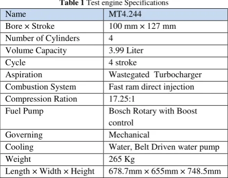
1. Engine Specification

In this study, the experiments were performed on an agricultural engine (MT4.244) produced by Motorsazan. Details of the engine’s specifications are given in Table 1.

Table 1 Test engine Specifications

Name MT4.244

Bore × Stroke 100 mm × 127 mm Number of Cylinders 4

Volume Capacity 3.99 Liter

Cycle 4 stroke

Aspiration Wastegated Turbocharger Combustion System Fast ram direct injection Compression Ration 17.25:1

Fuel Pump Bosch Rotary with Boost control

Governing Mechanical

Cooling Water, Belt Driven water pump

Weight 265 Kg

Length × Width × Height 678.7mm × 655mm × 748.5mm

2.2. Experimental set up

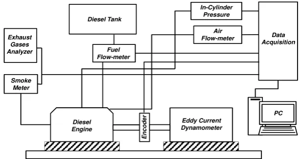
The study was carried out in the laboratory on an advanced fully computerized experimental engine test cell comprising of an eddy current dynamometer, in-cylinder pressure transducer, exhaust gas analyzer and soot meter. The schematic diagram of the experimental setup is shown in Fig. 1.

2.3 Experimentation and uncertainty error

In order to evaluate the performance and emissions, the experiments were conducted at four various injection timing [8°,4°,2° CA BTDC and 1° CA ATDC(-8,-4,-2 and +1 degrees]. The experiments were carried out at 1400 rpm (maximum torque speed), 1700 rpm and 2000 rpm (maximum power speed) and at four various loads (25%, 50%, 75% and 100%). The atmospheric pressure, charge pressure and ambient humidity were recorded regularly during the tests. The engine was warmed up for about 30 min. The experimental data required for the evaluation of the performance parameters and emissions were recorded after the engine was reached steady-state operation, which realized easily by observing a constant cooling water temperature. The variation in the power, BSFC, in-cylinder peak pressure and exhaust emissions of CO2, CO, HC, NOx and Smoke were determined for each mentioned

(3)

operating conditions. It should be noted that all the tests were repeated three times. The complete

experimental data and uncertainties of the engine performance and emissions are shown in Table 2

Fig1.Schematic diagram of experimental setup

Diesel Engine

Eddy Current Dynamometer

Data Acquisition Exhaust

Gases Analyzer

Smoke Meter

Diesel Tank

Fuel Flow-meter

Air Flow-meter

E

n

c

o

d

e

r PC

In-Cylinder Pressure

Table 2 Experimental results and uncertainties of the engine performance and emissions

Parameter Inj. timing

Engine Speed

Engine

Load Power HC CO CO2 NOx Smoke BSFC

Peak Pressure

Dimension sec rpm % Hp ppm ppm % ppm mg/m3 g/kW.h Bar

Uncertainty

Error (%) 2.86 0.18 1 0.03 3.31 0.16 0.1 0.16 0.14 0.04 0.012

1 -8 2000 100% 69.11 15 302 11.5 1565 63.44 222 140.88

2 -8 2000 75% 51.83 17 250 9.2 1102 33.67 228.629 101.02 3 -8 2000 50% 34.55 12 220 6.8 591 17.78 241.5267 86.90

4 -8 2000 25% 17.27 7 150 3.2 131 9.6 606.35 68.67

5 -8 1700 100% 59.28 17 621 10.9 1577 98.63 233.56 134.32

6 -8 1700 75% 44.46 18 512 8.8 1293 38.12 241.21 100.12

7 -8 1700 50% 29.64 13 446 6.6 775 18.17 249.23 83.45

8 -8 1700 25% 14.82 8 333 3 236 12.12 533.91 63.87

9 -8 1400 100% 49.11 22 878 10.4 1598 309.6 245.73 130.41

10 -8 1400 75% 36.83 19 780 8.3 1466 43.65 248.13 98.75

11 -8 1400 50% 24.55 15 650 6.5 862 19.04 269.45 79.86

12 -8 1400 25% 12.27 10 460 2.8 411 14.68 657.26 58.43

13 -4 2000 100% 57.80 33 611 11.9 914 76.4 263.81 115.09

14 -4 2000 75% 43.35 21 555 9.68 638 44.82 271.53 96.16

15 -4 2000 50% 28.90 15 401 7.45 349 18.16 303.14 82.12

16 -4 2000 25% 5.78 10 333 3.6 113 14.3 761.31 67.93

17 -4 1700 100% 52.87 45 777 11.4 1085 143.15 246.89 109.09

(4)

International Journal of Automotive Engineering Vol. 2, Number 4, Oct 2012

3. Artificial Neural Network (ANN)

3.1. Neural Network Design

ANN is an approach inspired by brain structure and tries to simulate the brain processing capabilities. Haykin defines a neural network as a massively

Parallel distributed processor [13]. It has an inherent tendency for storing experimental knowledge and making it available for use. It resembles the human brain in two respects: the knowledge is acquired by the network through a learning process, and inter-neuron connection strengths known as synaptic weights are used to store the knowledge. Neural network operates like a ‘‘black box” model, and does not require detailed information about the system. Instead, it learns the relationship between the 18 -4 1700 75% 39.34 30 643 9.33 823 46.12 259.63 89.81 19 -4 1700 50% 26.16 19 518 7.1 428 19.03 271.12 79.43 20 -4 1700 25% 8.01 10 411 3.5 188 14.88 790.54 62.12 21 -4 1400 100% 46.32 57 933 11.1 1135 225.8 254.34 104.07 22 -4 1400 75% 34.74 37 823 9 957 49.74 297.21 81.08 23 -4 1400 50% 23.16 22 708 6.8 608 19.35 323.90 67.23 24 -4 1400 25% 11.58 11 483 3.3 361 15.2 820.43 55.56 25 -2 2000 100% 55.29 39 799 12.35 691 108.2 261.12 101.09 26 -2 2000 75% 41.46 25 601 10.18 508 46.58 271.65 92.87 27 -2 2000 50% 27.64 19 483 7.77 258 19.96 315.11 78.52 28 -2 2000 25% 5.52 11 397 4.02 97 14.97 853.81 65.93 29 -2 1700 100% 49.49 68 871 12.1 739 198.32 267.43 98.40 30 -2 1700 75% 37.02 37 699 9.81 608 49.33 278.21 81.28 31 -2 1700 50% 25.63 25 566 7.48 304 21.22 323.09 73.52 32 -2 1700 25% 4.80 12 454 3.85 146 15.43 878.32 60.49 33 -2 1400 100% 43.98 95 978 11.9 858 295 296.59 94.92 34 -2 1400 75% 32.98 54 888 9.5 681 54.75 339.39 74.38 35 -2 1400 50% 21.99 31 762 7.1 437 23.02 369.98 66.09 36 -2 1400 25% 10.99 13 498 3.7 308 15.98 907.59 50.02 37 1 2000 100% 51.73 51 841 13.42 500 152.7 290.53 90.29 38 1 2000 75% 38.79 32 691 10.66 373 61.95 296.97 87.08 39 1 2000 50% 25.86 26 588 8.17 242 22.31 334.48 74.27

40 1 2000 25% 5.17 12 444 4.4 75 15.49 978.31 61.85

41 1 1700 100% 47.35 86 921 13.1 541 237.43 302.45 88.54 42 1 1700 75% 35.07 45 765 10.4 444 78.81 313.32 78.63 43 1 1700 50% 23.32 35 642 7.93 269 25.52 346.15 67.34 44 1 1700 25% 4.48 14 488 4.1 111 15.92 992.63 55.12 45 1 1400 100% 41.92 114 1009 12.34 639 391.45 329.95 85.78 46 1 1400 75% 31.44 64 909 9.85 531 91.88 371.82 73.23 47 1 1400 50% 20.96 45 818 7.3 379 27.04 404.03 64.65 48 1 1400 25% 10.48 15 513 3.9 255 16.33 1020.43 48.19

(5)

Fig2.The architecture of proposed ANN model for the engine.

Input parameters and the controlled and uncontrolled variables by studying previously recorded data, in a similar way that a non regression might be performed. Another advantage of using ANN is their ability to handle large and complex systems with many interrelated parameters. They simply ignore excess input data that are of minimal significance and concentrate instead on the more important inputs [14].

The learning-algorithm was used back propagation (BP), one of the most popular learning algorithms [15, 16]. Success in the algorithms depends on the user dependent parameters learning rate and momentum constant. Faster algorithms such as conjugate gradient, quasi-Newton, and Levenberg Marquardt (LM) use standard numerical optimization techniques. These algorithms eliminate some of the disadvantages mentioned above. In this case model

was trained with ‘‘Levenberg

optimization” learning algorithm. The Levenberg Marquardt algorithm is based on approaching second order training speeds without having t

of Hessian matrix [16].

MATLAB 7.0 was applied in all the stages of developed model including training and testing of the network. In this study ANN having an input layer with three neurons for each input factor (Injection timing, Engine loads and Engine speeds) and an output layer with eight neurons (NOx, Soot, HC, CO2, CO, Peak Pressure, Power and BSFC). One of the most important tasks in ANN studies is to choose the optimal network architecture which is related to the activation function and the number of neurons in hidden layer. Generally, the trial-and

is used. In this study, the optimal architecture of the network was obtained by trying different activation function and number of neurons. The performance of

The architecture of proposed ANN model for the engine.

parameters and the controlled and uncontrolled variables by studying previously recorded data, in a similar way that a non-linear regression might be performed. Another advantage of using ANN is their ability to handle large and interrelated parameters. They simply ignore excess input data that are of ficance and concentrate instead on the

algorithm was used back

propagation (BP), one of the most popular learning-16]. Success in the algorithms depends on the user dependent parameters learning rate and momentum constant. Faster algorithms such Newton, and Levenberg– Marquardt (LM) use standard numerical optimization

orithms eliminate some of the disadvantages mentioned above. In this case model

was trained with ‘‘Levenberg–Marquardt

optimization” learning algorithm. The Levenberg– Marquardt algorithm is based on approaching second-order training speeds without having the computation

MATLAB 7.0 was applied in all the stages of developed model including training and testing of the network. In this study ANN having an input layer with three neurons for each input factor (Injection timing, Engine loads and Engine speeds) and an er with eight neurons (NOx, Soot, HC, CO2, CO, Peak Pressure, Power and BSFC). One of the most important tasks in ANN studies is to choose the optimal network architecture which is related to the activation function and the number of neurons in and-error approach is used. In this study, the optimal architecture of the network was obtained by trying different activation function and number of neurons. The performance of

each network was checked by correlation coefficient (R) and is defined as follows:

The goal is to maximize correlation coefficient to obtain a network with the best generalization. R values were calculated for many different network models. Based on this analysis, the optimal architecture of the ANN was constructed as 3 NN and activation function in hidden layer and output layer both were ‘logsig’. The architecture of proposed ANN model is shown in Fig. 2

In the present work, 48 patterns were obtain from the experiments by changing the process parameters. Inputs and outputs have been normalized in the range of 0–1. Inputs for the ANN (process parameters) were the injection timing, engine loads and engine speeds and the outputs were shown in the Fig. 2

3.2 Evaluation of Results and D

An ANN was developed based on this experimental work to predict the missed data and avoid spending excessive time running experimental tests. The results showed that the training algorithm of Back Propagation was sufficient for predicting brake power, volumetric efficiency, peak pressure, specific fuel consumption and exhaust gas components for different engine load, speed and injection timing. For this purpose 40 patterns of the experimental results were used fo

model and 8 patterns were not applied to the model and were used for testing.

R₁∑ t o

∑ o

each network was checked by correlation coefficient

The goal is to maximize correlation coefficient to obtain a network with the best generalization. R values were calculated for many different network s analysis, the optimal architecture of the ANN was constructed as 3–15–8 NN and activation function in hidden layer and output layer both were ‘logsig’. The architecture of proposed

In the present work, 48 patterns were obtained from the experiments by changing the process parameters. Inputs and outputs have been normalized 1. Inputs for the ANN (process parameters) were the injection timing, engine loads and engine speeds and the outputs were shown in the

Discussion

An ANN was developed based on this experimental work to predict the missed data and avoid spending excessive time running experimental tests. The results showed that the training algorithm as sufficient for predicting brake power, volumetric efficiency, peak pressure, fic fuel consumption and exhaust gas components for different engine load, speed and injection timing. For this purpose 40 patterns of the experimental results were used for training the ANN model and 8 patterns were not applied to the model

1

(6)

211 Artificial Neural Network Based Multi-Objective…..

International Journal of Automotive Engineering Vol. 2, Number 4, Oct 2012 The Comparisons of the ANN-predicted results

and experimental (actual) results are indicated in Figs. 3 and 4. As mentioned before the criterion R was selected to evaluate the networks to find the best activation function and number of neuron. Linear regression analyses were carried out to investigate the network response in more detail. Correlation coefficients of 0.9902, 0.993, 0.998, 0.9916, 0.9923, 0.9951, 0.9921 and 0.9908 were obtained for the HC, CO2, CO, NOx, smoke, power, BSFC, peak pressure at the training stage. It is clear that the correlation coefficients for all output are close to unity indicating the good accuracy of the developed model. Thus, this ANN model can be used to predict emission and performance parameter for diesel engine with adequate accuracy.

3.3. Formulation

Hidden and output layers with ‘log-sigmoid’ transfer function were used to predict output. The log-sigmoid transfer function was:

Where x is the weighted sum of the input. To determine the emission parameters, bsfc, power and peak pressure. Equations 3 to 10 in Table 3 were derived from ANN. By using these equations similarly, performance and exhaust emissions of the diesel engine will be calculated.

Where f (i = 1, 2, 3... 15) can be calculated using:

Where

to

calculate as follows:

Where, the constants (Cji) are given in Table 4. For LM algorithm with 14 neurons and I, L and N are injection timing, speed and load, respectively. It should be noticed that in Equations 3-10, When using the equations in Table 4, I, N and L values are normalized by dividing them by 10, 2100 and 75 respectively. For outputs HC, CO, CO, NOx, Smoke, BSFC and PP values need to be multiplied by 120 , 1100, 15, 1600, 400, 1050 and 150, respectively.

Fig3.Comparisons of the ANN-predicted results and experimental (actual) results for Power, BSFC and Peak Pressure at test stage

R² = 0.9905

0 10 20 30 40 50 60 70

P

re

d

ic

te

d

P

o

w

e

r

(H

P

)

Experimental Power (HP)

R² = 0.9617

0 100 200 300 400 500 600 700 800 900

0 200 400 600 800 1000

P

re

d

ic

te

d

b

sf

c (

g

/K

w

.h

)

Experimental bsfc (g/Kw.h)

R² = 0.9816

60 70 80 90 100 110 120

P

re

d

ic

te

d

p

e

a

k

p

re

ss

u

re

(

P

a

)

Experimental peak pressure (Pa)

_{1 +}1 (2)

f_{1 + exp}1 (11)

! "!× $ + "!× % + "&!× ' + "! 12

(7)

Fig4.Comparisons of the ANN-predicted results and experimental (actual) results for NOx, HC, CO, CO2 and Smoke at test stage

Table 3 Derived equations from ANN

Power _{1 + e}_,..∗0₁_2.,∗0₃_.,∗0₄_2,.5.∗0₆_{2 ,.7∗0}₈_2,.&∗0₉_2,..∗0_:_2,.55∗01_;_2,.5<∗0₌_.5∗0_1>_,.<∗0₁₁_2.<.∗0₁₃_2,.∗0₁₄_2,.∗0₁₆_.??∗0₁₈_.? (3)

Bsfc _{1 + e}_&.∗0₁_,.,∗0₃_2,.&,∗0₄_.∗0₆_2..<∗0₈_2.&∗0₉_2,.7<∗0_:_2,.7∗01_;_{2 ,.&∗0}₌_2.?∗0_1>_2,.&∗0₁₁_,.?,∗0₁₃_2.,5∗0₁₄_2,..∗0₁₆_2.&∗0₁₈_. (4)

PP _{1 + e}_,.,?∗0₁_2,.∗0₃_,.<∗0₄_2,.5∗0₆_,..<∗0₈_,.?∗0₉_2,.∗0_:_2,.?∗01_;_{2 .5∗0}₌_.,∗0_1>_,.7∗0₁₁_2.<7∗0₁₃_2,.∗0₁₄_,.,<∗0₁₆_,.5,∗0₁₈_2,..? (5)

HC _{1 + e}_,.,<.∗0₁_,.∗0₃_.?∗0₄_{2 ,.57∗0}₆_{2 ,.5?∗0}₈_2,.5∗0₉_{2 ,.,&∗0}_:_,.?∗01 _;_.77∗0₌_2.,∗0_1>_2.<∗0₁₁_{2 ,.7&∗0}₁₃_,.7.∗0₁₄_2,.&,∗0₁₆_,.∗0₁₈_.7 (6)

CO _{1 + e}_,.∗0₁_2,.?∗0₃_.7,∗0₄_2,..∗0₆_2,..∗0₈_2,.77∗0₉_,.<&∗0_:_,.&&∗01_;_,.,<∗0₌_2.,∗0_1>_2.&.∗0₁₁_2,..,∗0₁₃_2,.,∗0₁₄_2,.,,∗0₁₆_,.,?∗0₁₈_,.7&? (7)

CO2 _{1 + e}_,.,∗0₁_2,.&∗0₃_.5&∗0₄_{2 .∗0}₆_{2 ,.∗0}₈_2,.&&∗0₉_2,.&∗0_:_2,.&.∗01 _;_2,...∗0₌_,.<?∗0_1>_2,.∗0₁₁_2,.5?∗0₁₃_{2 ,.∗0}₁₄_,.&<∗0₁₆_2.∗0₁₈_,., (8)

NOx _{1 + e}_,.7∗0₁_2.7∗0₃_2,.,7∗0₄_2,..<∗0₆_{2 .,∗0}₈_2,.5.∗0₉_2,.?5∗0_:_2.<∗01_;_2....∗0₌_.&∗0_1>_,.&∗0₁₁_2.5,∗0₁₃_2.7?∗0₁₄_2,.<∗0₁₆_2.5<∗0₁₈_.? (9)

Smoke _{1 + e}_,..,∗0₁_2,.,.∗0₃_&.?&∗0₄_2,.∗0₆_2.<&∗0₈_2.?∗0₉_.,<∗0_:_2,.5?∗01_;_{2 ,.<?∗0}₌_..7∗0_1>_2.5∗0₁₁_{2 .5&∗0}₁₃_.&∗0₁₄_2.∗0₁₆_2,.&∗0₁₈_&.?? (10)

R² = 0.9757

0 200 400 600 800 1000 1200

P

re

d

ic

te

d

N

O

x

(

p

m

)

Experimental NOx (ppm)

R² = 0.9821

0 10 20 30 40 50 60 70 80 90 100

0 20 40 60 80 100

P

re

d

ic

te

d

H

C

(

p

m

)

Experimental HC (ppm)

R² = 0.9784

0 200 400 600 800 1000 1200

P

re

d

ic

te

d

C

O

(

p

m

)

Experimental CO (ppm)

R² = 0.9719

0 2 4 6 8 10 12 14

0 2 4 6 8 10 12 14 16

P

re

d

ic

te

d

C

O

2

(

%

)

Experimental CO2 (%)

R² = 0.9842

0 50 100 150 200 250 300 350

P

re

d

ic

te

d

s

o

m

k

e

Experimental smoke

(8)

213 Artificial Neural Network Based Multi-Objective…..

International Journal of Automotive Engineering Vol. 2, Number 4, Oct 2012

4. Multi-objective optimization

Multi-objective optimization, which is also called multi criteria optimization, has been defined as finding a vector of decision variables satisfying constraints to give acceptable values to all objective functions. In general, it can be mathematically defined as Find the vector J∗= [∗ , ∗ , … , _K∗ ] to optimize:

Subject to m inequality constraints,

and p equality constraints:

where X∗∈ RN is the vector of decision or design variables and Fx ∈ RP is the vector of objective functions, which must each be either minimized or maximized [17].

A variety of approaches can be used to solve this problem. One popular approach is to combine those objectives into a single composite objective so that traditional mathematical programming methods can be applied. To this end, some sort of value or utility function needs to be identified according to the preference of one or multiple decision-makers. The simplest method is to assume independent preferences among those objectives and apply an additive utility function. On the other hand, instead of transforming the original problem into a single-objective one, the Pareto optimum concept based on non-dominance can be utilized. Maheshvari et al. used traditional method to optimize IC engine parameters and transformed the original problem into a single-objective one [18].

In many MOPs, the considered objectives are in conflict with each other. Therefore, it is impossible to gain a solution that optimizes each objective function concurrently. The answer such problems are a set of solutions, called Pareto optimal. But, before defining this term, the concept of dominant must be introduced. Assume that x1 and x2 are vectors in n-dimensional space and f is a function. x1 dominates x2 if the following conditions satisfy:

Pareto optimal is a solution which is not dominated by any other solution in the solution space. The main characteristic of the Pareto optimal solution is that it cannot be improved with respect to an objective unless deteriorating at least one other objective. A set of all these non-dominated solutions is called Pareto optimal set and the corresponding objective function values in the objective space are the Pareto front. Finding the Pareto front, which

consists of Pareto optimum solutions, is the major goal in MOPs.

In order to deal with this multi-objective optimization problem, a multi-objective evolutionary algorithm is proposed. To generate a Pareto-optimal, the powerful multi-objective evolutionary algorithm, Non-dominated Sorting Genetic Algorithm (NSGA-II), was used. The NSGA-II makes use of a fast non-dominated sorting approach, elitist strategy, and a crowded comparison operator to create Pareto-optimal solutions. First a random parent population is created. Binary tournament selection, recombination, and mutation operators are used to create a child population. Then, a combined parent and child population is formed. This allows parent solutions to be compared with the child population, thereby ensuring elitism. The population is sorted according to non-domination. The new same size parent population is formed according to non-domination ranks and crowded comparison operator. This population is now used for selection, crossover and mutation to create a new population [19].

5. Pareto optimization of power and overall

emissions using neural network models

In order to gain optimal power and overall emissions, the neural network models obtained in the previous sections are now used in a multi-objective optimization procedure. The two objectives in this study are overall engine exhaust emissions and power to be simultaneously optimized with respect to the design variables, namely injection timing, engine speed and engine load. The overall exhaust emission was defined as below [18].

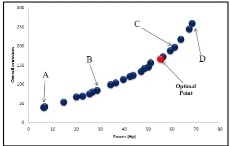
The corresponding Pareto front of two objectives power and overall emissions has been shown in Fig. 5. It is clear from this figure that choosing appropriate values for engine speed, load and injection timing for obtaining a better value of one objective would cause a worse value of another objective.

Four sections, A, B, C and D, can be seen from Fig. 5 that illustrate important optimal design facts. Area between sections A and B exhibits an increase of power with a small change in overall emissions according to its slip 1.98. Area between sections C and D exhibits a significant increase of overall emission while power (slip 8.86) is not increases

[R, R, … , RU]W, 13

Y! ≤ 0 \ 1 ]^ _ 14

ℎb 0 c 1 ]^ d 15

fR! ≤ R!ijk ∀\ 1 , … , h R! < R! ∃\ 1 , … , h

n ₁₆

pqriss _\tt\^jt _%p%p

uv+

"p "puv

+_"p"p

uv+

w" w"uv

+_{x_^h}x_^h

uv

17

(9)

significantly. Therefore, changing the injection timing, engine speed and engine load as decision variables should be in such a way that power and overall emission lies between sections B and C of the Pareto optimal front which has a slip of 3.45.

As shown in Fig. 5, the optimal result was selected and has the coordinates of (50,143). This

point corresponds to Power of 50 HP and overall emissions of 143. In other words, with the engine speed 1943 rpm, load of 240.82 N.m. and injection timing -7.8 ( 7.8 bTDC), the best solution was obtained

Fig5.Optimization result (Pareto front)

Table 4 The weights and biases between input layer and hidden layer for Eqs. (3) to (10).

! "!× $ + "!× % + "&!× ' + "!

i "_! "_! "_&! "_!

1 -8.0268 2.5952 12.6505 -3.1785

2 -4.2729 -27.6237 10.7672 19.6299

3 -3.5191 0.59379 -7.7725 4.6328

4 1.8233 7.9999 22.3282 -13.0801

5 -10.5491 -34.8195 0.10597 29.4396

6 11.2742 27.1059 2.1041 -23.5179

7 -8.5576 26.9746 3.7775 -33.653

8 -3.4063 34.4069 7.185 -34.2456

9 -7.0547 -6.9283 6.3134 -5.3252

10 -7.7067 -36.7574 4.8087 22.6632

11 12.9156 30.3336 -1.6584 -17.4314

12 -8.7067 -33.0747 6.3342 18.8497

13 13.5601 -11.4703 -0.19769 18.4414

14 0.0089625 -47.7151 5.3141 27.2334

15 -1.3715 -19.8066 11.6078 -3.2733

6. Conclusion

In this investigation, It is assessed the influence of three key factors of engine loads, speeds and injection timing. After getting data from experimental tests by varying the engine speed, load and injection timing,

using ANN to modeling the engine to predict the performance and emissions for all operating conditions. This reduces the experimental efforts and hence can serve as an effective tool for predicting the performance of the engine and emission characteristics under various operating conditions. It is considered that the ANN results are very good and

(10)

International Journal of Automotive Engineering Vol. 2, Number 4, Oct 2012 R values in this model are very close to one. Results

showed Correlation coefficients of 0.9902, 0.993, 0.998, 0.9916, 0.9923, 0.9951, 0.9921 and 0.9908 were obtained for the HC, CO2, CO, NOx, smoke, power, BSFC, peak pressure at the training stage respectively. Then, by using NSGA II, the best solution was obtained to optimize the two objective functions minimum overall exhaust emissions and maximum engine power.

References

[1]. Payri F., Benajes J., Arregle J., Riesco J.M., (2006) Combustion and exhaust emissions in a heavy-duty diesel engine with increased premixed combustion phase by means of injection retarding. Oil & Gas Science and Technology 61:247–58.

[2]. Aktas A., Sekmen Y., (2008) The effects of advance fuel injection on engine performance and exhaust emissions of a diesel engine fueled with biodiesel. J Faculty Eng Architect Gazi Univ 23:196–208 [In Turkish].

[3]. Sayin C., Kadir U., Mustafa C., (2008) Influence of injection timing on the exhaust emissions of a dual fuel CI engine. Renewable Energy 33:1314–1323.

[4]. Sayin C., Ozsezen A.N., Mustafa Canakci M., (2010) The influence of operating parameters on the performance and emissions of a DI diesel engine using methanol-blended-diesel fuel. Fuel 89 1407–1414.

[5]. Parlak A., Islamoglu Y., Yasar H., Egrisogut A., (2006) Application of artificial neural network to predict specific fuel consumption and exhaust temperature for a diesel engine”, Applied Thermal Engineering 26:824–8.

[6]. Ghobadian B., Rahimi H., Nikbakht A., Najafi G., Yusaf T.F., (2009) Diesel engine performance and exhaust emission analysis using waste cooking biodiesel fuel with an artificial neural network. Renewable Energy 34:976–982.

[7]. Togun N.K., Baysec S., (2010) Prediction of torque and specific fuel consumption of a gasoline engine by using artificial neural networks. Applied Energy 87:349–355.

[8]. Shivakumar P., Srinivasa P., Shrinivasa B.R., (2011) Artificial Neural Network based prediction of performance and emission characteristics of a variable compression ratio CI engine using WCO as a biodiesel at different injection timings. Applied Energy 88:2344– 2354

[9]. Haupt R.L., Haupt S.E., (2004) Practical Genetic Algorithms. Second Edition. John Wiley & Sons.

[10]. Abraham A., Jain L., Goldberg R., (2005) Evolutionary Multiobjective Optimization. Springer-Verlag London Limited.

[11]. Coello C.A. (1999) A comprehensive survey of evolutionary-based multiobjective optimization techniques. Knowledge and Information Systems: An International Journal 3:269–308. [12]. Deb K., Agrawal S., Pratap A., Meyarivan T.

(2002) A fast and elitist multiobjective genetic algorithm: NSGA-II. IEEE Transactions on Evolutionary Computation 6 (2):182–197. [13]. Haykin S., (1994) Neural networks: a

comprehensive foundation. New York: Macmillan.

[14]. Hagan M.T., Demuth H.B., (1995) Neural network design. PWS Publishing Company. Boston, USA.

[15]. Muthukrishnan N., Paulo Davim J. (2009) Optimization of machining parameters of Al/SiC-MMC with ANOVA and ANN analysis. Journal of Materials Processing Technology 209:225-232.

[16]. Montano J.J., Palmer A., (2003) Numeric sensitivity analysis applied to feedforward neural networks. Neural Comput & Applic 12:119-125.

[17]. . Branke J., Deb K., Miettinen K., Słowinski R., (2008) Multiobjective optimization. Springer-Verlag Berlin Heidelberg.

[18]. Maheshwari N., Balaji C., Ramesh A., (2011) A nonlinear regression based multi-objective optimization of parameters based on experimental data from an IC engine fueled with biodiesel blends. Biomass and bioenergy 35:2171-2183

[19]. Nakayama H., Yun Y., Yoon M., (2009) Sequential Approximate Multiobjective Optimization Using Computational Intelligence. Springer-Verlag Berlin Heidelberg.