The modified BFGS method with new secant relation for
uncon-strained optimization problems
Razieh Dehghani∗
Faculty of Mathematics, Yazd University, Yazd, Iran.
E-mail: [email protected]
Mohammad Mehdi Hosseini
Faculty of Mathematics, Yazd University, Yazd, Iran.
E-mail: hosse−[email protected],
Narges Bidabadi
Faculty of Mathematics, Yazd University, Yazd, Iran.
E-mail: n−[email protected].
Abstract Using Taylor’s series we propose a modified secant relation to get a more accurate approximation of the second curvature of the objective function. Then, based on this modified secant relation we present a new BFGS method for solving unconstrained optimization problems. The proposed method make use of both gradient and func-tion values while the usual secant relafunc-tion uses only gradient values. Under appro-priate conditions, we show that the proposed method is globally convergent without needing convexity assumption on the objective function. Comparative results show computational efficiency of the proposed method in the sense of the Dolan-Mor´e performance profiles.
Keywords. Unconstrained optimization, Modified BFGS method, Global convergence. 2010 Mathematics Subject Classification. 90C30, 90C53, 49M37, 65K05.
1. Introduction
Consider the unconstrained nonlinear optimization problem
minf(x), x∈Rn, (1.1)
where,f :Rn→R,is twice continuously differentiable.
Notation 1. Throughout our work, we consider the following notations:
fk=f(xk), sk =xk+1−xk, gk=∇f(xk), yk=gk+1−gk, Gk+1=∇2f(xk+1).
Also,k.k is the Euclidean norm.
As we all know, Newton method based on the second order Taylor’s series approx-imation involves computation of the Hessian matrix of second order derivatives at
Received: 24 December 2017 ; Accepted: 27 October 2018.
∗Corresponding author.
each iteration. In practice it is often preferred to approximate the Hessian matrix (or sometimes its inverse) with a symmetric positive definite matrix through some effective procedure instead of its exact computation. This idea of approximating the Hessian with a symmetric positive definite matrix was first introduced by Davidon [7]. The class of methods that approximates Newton method by utilizing some symmetric positive definite approximation of the Hessian or the inverse Hessian instead of the corresponding exact value is termed as quasi-Newton methods.
The quasi-Newton methods possess a number of important theoretical properties (see [4], [5], [8], [9], [22] ), for example, quadratic termination, invariance under non-singular affine transformations, heredity of positive-definite updates, and generating identical iterate points with exact line searches (see [11]), locally and superlinearly convergence under mild conditions (see [8], [9]).
These methods generate a sequence{xk}by the iterative scheme
xk+1=xk+αkdk, (1.2)
where, αk > 0 is a step length and dk is the search direction obtained by solving Bkdk =−gk, whereBk is an approximation of the Hessian matrix of f atxk.
A famous class of quasi-Newton methods is the Broyden family [2] in which the Hessian updates are defined by
Bk+1=Bk−
BksksTkBk sT
kBksk
+yky
T k sT
kyk
+µwkwkT, wk = (sTkBksk)1/2[ yk sT
kyk
− Bksk
sT kBksk
],
whereµis a scalar andBk+1 satisfies the following standard secant relation:
Bk+1sk =yk. (1.3)
The popular BFGS, DFP and SR1 updates are obtained by settingµ= 0,µ= 1 and
µ= 1/(1−sTkBksk/sTkyk),respectively.
From the numerical experiment on the quasi-Newton methods, it is proved that the BFGS method is the most successful one among all the quasi-Newton methods. But the global convergence for general function f is still open even if it is convergent (global and superlinear) for convex minimization [1]-[3], [10]. Hence, it is very interesting to investigate whether there is any new quasi-Newton method that not only possess global convergence but also superior than the BFGS method from the computation point of view.
The usual secant relation employs only the gradients and the available function values are ignored. To overcome this problem, several researchers have modified the usual secant relation (1.3) to make full use of both the gradient and function values (see [25]-[29]).
Zhang and Xu [29], using Taylor’s series, modified usual secant equation (1.3) as follows:
Bk+1sk =yk, yk =yk+ ϑk
kskk2
sk, (1.4)
with
ϑk = 6(fk−fk+1) + 3(gk+gk+1)Tsk. (1.5)
A merit of the new modified secant method can be seen from the following theorem [29].
Theorem 1.1. Assume that the functions f(x) are smooth enough and yk is de-fined by (1.4). Ifkskk is sufficiently small, then we have
sTk(Gk+1sk−yk) =O(ksk k4), sTk(Gk+1sk−yk) =O(ksk k3).
Resently, Yabe and Takano [27] extended the modified secant relation (1.4) by mul-tiplying a fixed parameterρ≥0,as follows:
Bk+1sk =zk, zk=yk+ρ ϑk
kskk2 sk,
whereϑk is given by (1.5).
Theorem 1.1, demonstrate ifkskk > 1, the standard secant relation is expected to
be more accurate than the modified secant relation (1.4). In this case, the use of (1.4)) does not seem to be suitable. To overcome these problems, Peyghami et al. [21] modified (1.4) as follows:
Bk+1sk =wk, wk =yk+ρk ϑk
kskk2
sk, (1.6)
with
ρk= min(ρmax, a b+kskkm
), (1.7)
wherea, b, ρmax andmis a nonnegative integer.
secant relation. In section 3, we investigate the global convergence of the proposed method. Finally, in section 4, we report some numerical results.
2. Proposed modified quasi-Newton method
Consider the following auxiliary function
fk(x) =f(x) + rk
2(x−xk)
T(x−x
k). (2.1)
Obviously the functionsfk andf have the same value inxk.
By using (2.1), we have
Bk+sk=yk∗, y
∗
k=yk+rksk. (2.2)
Clearly, different choices of therk in (2.2) define a variety of secant relation. Here,
we introduce a reasonablerk,that leads a new secant relation.
Using the Taylor formula for the functionsf(x), we obtain
fk'fk+1−gTk+1sk+21sTkGk+1sk−16Pni,j,l=1 ∂3fk+1
∂xi∂xj∂xls
i ks j ks l k +1 24 Pn i,j,k,l=1
∂4f
k+1
∂xi∂xj∂xk∂xls
i ks j ks k ks l k, (2.3) sT
kgk'sTkgk+1−skTGk+1sk+12Pni,j,l=1 ∂3fk+1
∂xi∂xj∂xls
isjsl
−1 6
Pn i,j,d,l=1
∂4f
k+1
∂xi∂xj∂xd∂xls
i ks j ks d ks l k, (2.4)
sTkGksk'sTkGk+1sk− n
X
i,j,l=1
∂3f
k+1
∂xi∂xj∂xls i ks j ks l k+ 1 2 n X i,j,d,l=1
∂4f
k+1
∂xi∂xj∂xd∂xl∂s i ks j ks d ks l k. (2.5)
Cancellation ofPn i,j,l=1
∂3fk+1
∂xi∂xj∂xls
i ks j ks l k and Pn i,j,d,l=1
∂4fk+1
∂xi∂xj∂xd∂xl∂s
i ks
j ks
d
kslk,from (2.3),
(2.4) and (2.5) yields,
sTkGk+1sk'12(fk−fk+1) + 6(gk+gk+1)Tsk+sTkGksk. (2.6)
SinceBk+1 approximateGk+1=∇2f(xk+1),we have
sTkBk+1sk=sTkyk+ 12(fk−fk+1) + 7gTksk+ 5gTk+1sk+sTkBksk. (2.7)
On the other hand, multiplying both sides of (2.2) bysk, we get
sTkBk+1sk=sTkyk+rksTksk. (2.8)
The relation (2.7), together with (2.8), result in
rk=
θk
kskk2
, θk= 12(fk−fk+1) + 7gkTsk+ 5gkT+1sk+sTkBksk. (2.9)
Now, Based on the above observation, we can modify the secant relation (1.3) as follows
with
y∗k=yk+
θk
kskk2
sk, θk= 12(fk−fk+1) + 7gkTsk+ 5gkT+1sk+sTkBksk. (2.11)
A merit of the new modified secant method is revealed by the following result.
Theorem 2.1. Assume that the functionsf is smooth enough andy∗kis defined by (2.11).
Ifkskkis sufficiently small, then we have
sTk(Gk+1sk−y∗k) =O(kskk5),
sTk(Gk+1sk−yk) =O(kskk4),
and
sTk(Gk+1sk−yk) =O(kskk3).
Proof. The result follows immediately from (2.3), (2.4) and (2.5) (for details, see Theorem
2.1 of [25].
Theorem 2.1 implies that the quantitysT ky
∗
kgenerated by the modified secant method
ap-proximates the second-order curvaturesTkGk+1skwith a higher accuracy respect to quantity
sT
kykandsTkyk.
Obviously, determine vk by (2.11) require expensive computations at each iteration
(be-cause of the matrix-vector products), especially for large problems. We are going to propose an effective approach to to reduce the level of computation to determiningvk.
We know direction search computed by
dk=−B
−1
k gk. (2.12)
On the other hand, using (1.2), we get
sk=αkdk. (2.13)
From (2.12) and (2.13), we obtain
Bksk=−αkgk. (2.14)
Also, we know thatBk satisfies
Bksk−1=yk−1. (2.15)
Using (2.14) and (2.15), the relation (2.11) can be written as
yk∗=yk+
θk
kskk2
sk, θk= 12(fk−fk+1) + 7gTksk+ 5gTk+1sk−α2kd T
kgk. (2.16)
Hence, we can be written as the secant relation (2.10) as follows:
Bk+1sk=y∗k, y
∗
k=yk+ρk
θk
kskk2
sk, (2.17)
whereρkandθkare given by (1.7) and (2.16) respectively.
Clearly, this relation is considerably less expensive than that given in (2.10), especially for large scale problems.
overcome this, we using the idea in [18] and updateBk+1 by the following rule:
Bk+1= (
Bk− BksksT
kBk
sT
kBksk +
y∗ky∗kT
sT ky∗k
, sTky ∗ k kskk2 ≥δ,
Bk, otherwise.
(2.18)
An attractive property of this update forBkis that
yk∗ T
sk>0, (2.19)
which guarantees the positive definiteness of matrixBk.
We can now give a new BFGS algorithm using our new secant relation as follows.
Algorithm 1: A modified BFGS method.
Step 1: Give ε as a tolerance for convergence, σ1 ∈ (0,1), σ2 ∈ (σ1,1), a starting point
x0 ∈Rn,and a positive definite matrixB0.Setk= 0.
Step 2: Ifkgkk< εthen stop.
Step 3: Compute a search directiondk: SolveBkdk=−gk.
Step 4: Computeαkby using the following Wolfe conditions:
f(xk+αkdk)≤f(xk) +σ1αkgkTdk, (2.20)
and
g(xk+αkdk)Tdk≥σ2g(xk)Tdk. (2.21)
Step 5: Setxk+1=xk+αkdk. Computey∗kby (2.17). UpdateBk+1by (2.18).
Step 6: Setk=k+ 1 and go to Step 2.
Next, we will investigate the global and asymptotic superlinear convergence of the proposed algorithm.
3. Convergence analysis
In order to establish the global convergence of the Algorithm 1, we need some commonly used assumptions.
Assumption A. The level setD={x|f(x)≤f(x0)}is bounded, wherex0 is the starting point of Algorithm 1.
Assumption B. In an open setN containingD, there exists a constantL >0 such that
kg(x)−g(y)k ≤Lkx−yk,∀x, y∈N.
It is clear that assumptions A and B imply that there exists a positive constantγsuch that
From Assumption A and the Wolfe conditions,{f(xk)}is a non-increasing sequence, which
ensures{xk} ⊂D and the existence ofx∗such that
lim
k→∞f(xk) =f(x ∗
). (3.2)
To establish convergence of Algorithm 1, we first provide some lemmas.
Lemma 3.1. Let f satisfy assumptions A and B, and {xk} be generated by Algorithm
1 and there exist constantsa1anda2 such that,
kBkskk ≤a1kskkandskTBksk≥a2kskk2, (3.3)
for infinitelyk, then we have
lim inf
k→∞ g(xk) = 0. (3.4)
Proof. From (3.3) and the relationgk=−Bkdk we have
dTkBkdk≥a2kdkk2, a2kdkk ≤ kgkk ≤a1kdkk. (3.5)
Let Λ be the set of indicesksuch that (3.5) holds. By using (2.21) and Assumption B, we have
Lαkkdkk2≥(gk+1−gk)Tdk≥(1−σ2)gkTdk. (3.6)
This implies that, for anyk∈Λ,
αk≥
(1−δ)gkTdk
Lkdkk2
= (1−δ)d
T kBkdk
Lkdkk2
=(1−δ)a2
L . (3.7)
On the other hand, from (3.2), we obtain
∞ X
k=1
(fk−fk+1) = lim N→∞
N
X
k=1
(fk−fk+1) = lim
N→∞(f(x1)−fN) =f(x1)−f ∗ , which yields ∞ X k=1
(fk−fk+1)<∞,
Using (2.20), we get
∞ X
k=1
αkgTkdk<∞,
which ensures
lim
k→∞αkg
T kdk= 0,
this together with (3.7) lead to
lim
k∈Λ,k→∞d
T
kBkdk= lim k∈Λ,k→∞−g
T kdk= 0,
which along with (3.5), yields (3.4).
Lemma 3.2.(Theorem 2.1 of [3]) Suppose that there are positive constantsmandM such that for allk≥0
sTky
∗
k
kskk2
≥mand ky ∗
kk2
sT ky
∗
k
≤M. (3.8)
Now, we prove the global convergence for Algorithm 1.
Theorem 3.1. Let f satisfies in assumption A and B, and {xk} be generated by
Algo-rithm 1. Then, we have
lim inf
k→∞ g(xk) = 0. (3.9)
Proof. In view of Lemma 3.1, sufficiently show that (3.3) holds for infinitelyk.
LetK={k| sTky ∗ k
kskk2 ≥δ}.IfKis a finite set, then from (2.18)Bk,is a constant matrix after some finite iterations, clearly (3.3) holds for all largek.
Now, supposeKis a infinite set, then we have
sTky
∗
k≥δkskk2, ∀k∈K. (3.10)
By the definitions ofy∗kand Assumption B, it is easy to see that
ky∗kk
2
sT ky
∗
k
≤M.
whereM >0 is a constant. Applying Lemma 3.2 to the subsequence{Bk}k∈K,there exist,
constantsa1 >0 anda2 >0 such that (3.3) holds for infinitely manyk. Then, Lemma 3.1
completes the proof.
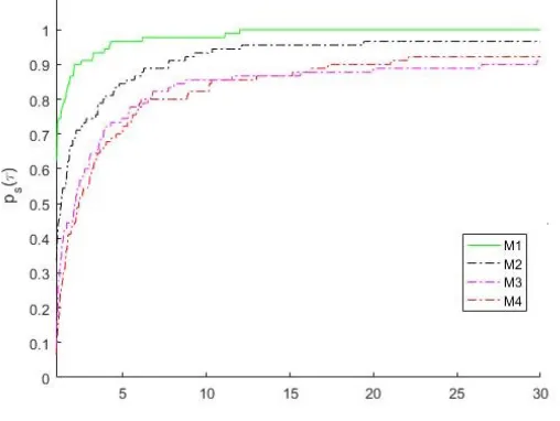
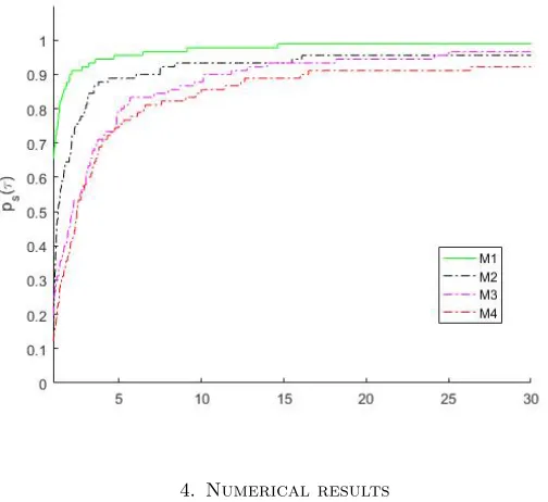
Figure 2. Total number of function evaluations performance profiles
for the Algorithms.
4. Numerical results
We compare the performance of the following four methods on some unconstrained opti-mization problems:
M1: proposed method (Algorithm 1) witha=b=ρmax= 1, m= 10.
M2: the modified BFGS of Peyghami et al. using (1.6) [21] witha=b=ρmax= 1, m= 10.
M3: the modified BFGS method of Zhang and Xu using (1.4) [29]. M4:the usual BFGS method using (1.3) [3].
We have tested all the considered algorithms on 120 test problems from CUTEr library [16]. A summary of these problems are given in Table 1 of [8]. All codes were written in Matlab 2012 and run on a PC with CPU Intel(R) Core(TM) i5-4200 3.6 GHz, 4 GB of RAM memory and Centos 6.2 server Linux operating system.
In the four algorithms, the initial matrix is set to be the identity matrix, and the step length αk was computed satisfying the Wolfe conditions, with σ1 = 0.01, σ2 = 0.9 and
ε= 10−6.In Algorithm 1 we setδ= 10−6.
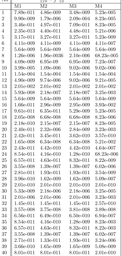
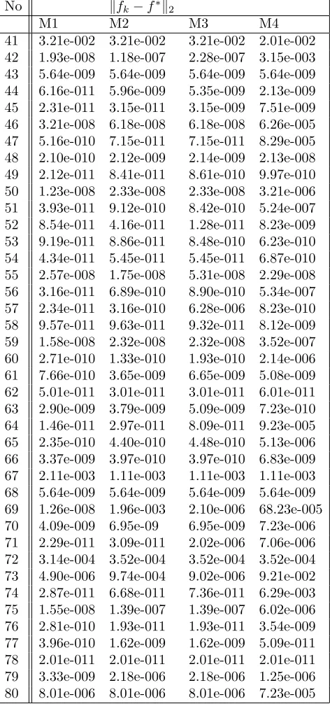
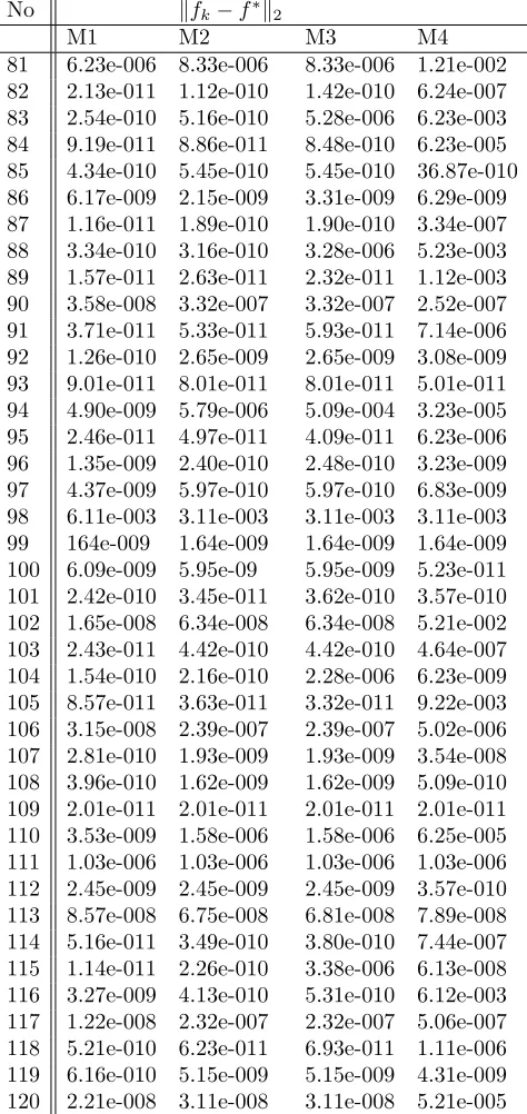
Tables 1-3 in the appendix list estimation errors of these algorithms, wheref∗ stand for optimal value objective function.
We used the performance profiles of Dolan and Mo´re (see [12]) to evaluate performance of these two algorithms with respect to the number of iterations and the total number of function and gradient evaluations computed as
whereNf andNg,respectively denote the number of function and gradient evaluations (note
that to account for the higher cost ofNg,as compared toNf,the former is multiplied byn).
Figures 1 and 2 demonstrate the results of the comparisons. From these figures, it is clearly observed that the proposed method (M1) is the most efficient for solving these 120 test problems.
5. Conclusion
We propose a modified secant relation to get a more accurate approximation of the sec-ond curvature of the objective function. Then, based on the proposed secant relation, we presented a modified BFGS for solving unconstrained optimization problem. The global convergence of all the proposed methods was established, under suitable assumptions. Nu-merical results on the collection of problems from the CUTEr library showed the proposed method to be more efficient as compared to several proposed BFGS methods in the literature.
Acknowledgements
We would like to thank the referees and the associate editor, whose very helpful sugges-tions led to much improvement of this paper.
References
[1] C. G. Broyden,A class of methods for solving nonlinear simultaneous equations, Math. Comp.,19(1965), 577–593.
[2] C. G. Broyden,The convergence of a class of double rank minimization algorithms-Part 2: The new algorithm, J. Inst. Math. Appl.,6(1970), 222–231.
[3] R. Byrd and J. Nocedal,A tool for the analysis of quasi-Newton methods with application to unconstrained minimization, SIAM J. Numerical Anal.,26(1989), 727–739.
[4] R. Byrd, J. Nocedal, and Y. Yuan,Global convergence of a class of quasi-Newton methods on convex problems, SIAM J. Numer. Analysis,24(1987), 1171–1189.
[5] A. R. Conn, N. Gould, and Ph. L. Toint,Convergence of quasi-Newton matrices generated by the symmetric rank one update, Math. Programming,50(1991), 177–195.
[6] Y. Dai, Convergence properties of the BFGS algorithm, SIAM J. Optim., 13 (2003), 693–701.
[7] W. C. Davidon,Variable metric methods for minimization, Argonne National Labs Re-port, ANL-5990.
[8] R. Dehghani, N. Bidabadi, and M. M. Hosseini,A new modied BFGS method for un-constrained optimization problems, Computational and Applied Mathematics,37(2018), 5113-5125.
[9] J. E. Dennis and J. J. Mor´e, Quasi-Newton methods, motivation and theory, SIAM Review,19(1977), 46–89.
[10] J. E. Dennis and R. B. Schnabel,Numerical methods for unconstrained optimization and nonlinear equations, Prentice-Hall, Englewood Cliffs, New Jersey, 1983.
[11] L. C. W. Dixon,Quasi-Newton algorithms generate identical points, Math. Programming,
2(1972), 383–387.
[12] E. Dolan and J. J. Mor´e,Benchmarking optimization software with performance profiles, Math. Program.,91(2002), 201–213.
[13] R. Fletcher,A new approach to variable metric algorithms, Comput.,13(1970), 317–322. [14] J. A. Ford and A. F. Saadallah,On the construction of minimisation methods of
quasi-Newton type, J. Comput. Appl. Math.,20(1987), 239–246.
[16] N. I. M. Gould, D. Orban, and Ph. L. Toint,A constrained and unconstrained testing environment, revisited, ACM Trans. Math. Softw.,29(4) (2003), 373–394.
[17] A. Griewank, The global convergence of partioned BFGS on problems with convex de-compositons and Lipschitzian gradients, Math. Program.,50(1991), 141–175.
[18] D. H. Li and M. Fukushima,On the global convergence of BFGS method for nonconvex unconstrained optimization problems, SIAM Journal on Optimization,11(2001), 1054– 1064.
[19] D. H. Li and M. Fukushima, A modified BFGS method and its global convergence in nonconvex minimization, J. Comput. Appl. Math.,129(2001), 15–35.
[20] W. F. Mascarenhas, The BFGS method with exact line searches fails for non-convex objective functions, Math. Program.,99(2004), 49–61.
[21] M. R. Peyghami, H. Ahmadzadeh, and A. Fazli, A new class of efficient and globally convergent conjugate gradient methods in the Dai-Liao family, Optimization Methods and Software,30(4) (2015), 843–863.
[22] M. J. D. Powell, Some global convergence properties of a variable metric algorithm for minimization without exact line searches, In: Cottle, R.W., Lemke, C.E. (eds.), Nonlinear Programming, SIAMAMS Proceedings, vol. IX. SIAM, Philadelphia, 1976.
[23] D. F. Shanno,Conditioning of quasi-Newton methods for function minimization, Math. Comp.,24(1970), 647–656.
[24] Ph. L. Toint,Global convergence of the partioned BFGS algorithm for convex partially separable opertimization, Math. Program.,36(1986), 290–306.
[25] Z. Wei, G. Li, and L. Qi, New quasi-Newton methods for unconstrained optimization problems, Appl. Math. Comput.,175(2006), 1156–1188.
[26] G. Yuan and Z. Wei,Convergence analysis of a modified BFGS method on convex mini-mizations, Computational Optimization and Applications,47(2010), 237–255.
[27] H. Yabe and M. Takano,Global convergence properties of nonlinear conjugate gradient methods with modified secant condition, Comput. Optim. Appl.,28(2004), 203–225. [28] J. Z. Zhang, N. Y. Deng, and L. H. Chen,New quasi-Newton equation and related methods
for unconstrained optimization, J. Optim. Theory Appl.,102(1999), 147–167.
[29] J. Z. Zhang and C. X. Xu,Properties and numerical performance of quasi-Newton meth-ods with modified quasi-Newton equation, J. Comput. Appl. Math.,137(2001), 269–278. [30] D. T. Zhu, Nonmonotone backtracking inexact quasi-Newton algorithms for solving
smooth nonlinear equations, Appl. Math. Comput.,161(2005), 875–895.
Table 1. Test results for the two algorithms.
No kfk−f∗k2
M1 M2 M3 M4
Table 2. Test results for the two algorithms.
No kfk−f∗k2
M1 M2 M3 M4
Table 3. Test results for the two algorithms.
No kfk−f∗k2
M1 M2 M3 M4