Distributed Support Vector Machine With Graphics Processing Units

(1)

University of New Orleans University of New Orleans

ScholarWorks@UNO

University of New Orleans Theses and

Dissertations Dissertations and Theses

8-6-2009

Distributed Support Vector Machine With Graphics Processing

Units

Hang Zhang

University of New Orleans

Follow this and additional works at: https://scholarworks.uno.edu/td

Recommended Citation Recommended Citation

Zhang, Hang, "Distributed Support Vector Machine With Graphics Processing Units" (2009). University of New Orleans Theses and Dissertations. 991.

https://scholarworks.uno.edu/td/991

This Thesis is protected by copyright and/or related rights. It has been brought to you by ScholarWorks@UNO with permission from the rights-holder(s). You are free to use this Thesis in any way that is permitted by the copyright and related rights legislation that applies to your use. For other uses you need to obtain permission from the rights-holder(s) directly, unless additional rights are indicated by a Creative Commons license in the record and/or on the work itself.

(2)

Distributed Support Vector Machine With Graphics Processing Units

A Thesis

Submitted to the Graduate Faculty of the University of New Orleans in partial fulfillment of the requirements for the degree of

Master of Science in

Computer Science Bioinformatics

(3)

ii

(4)

iii

Acknowledgments

First and foremost, I want to thank my advisor Dr. Stephen Winters-Hilt. His endless support and wisdom helped me to finish this thesis. His enthusiasm for Bioinformatics was contagious— and I definitely caught it. His depth of knowledge and very precise academic guidance brought me to an understanding of machine learning algorithm in depth.

I would also like to thank Murat Eren. He was always ready to give me hints whenever I needed them. We learned SVM algorithm together and his integral knowledge helped me understand SVM quicker.

My bioinformatics group members helped me with their smart ideas and enlightened the thoughts behind my thesis. For their help I am deeply grateful.

I would like to express my gratitude to all those who helped to make this thesis a reality: Vico Marziale, Fangfang Liu, George Voulgarakis, Guorong Xu. With their aid and encouragement, I made it through the thesis-writing process.

(5)

iv

List of Figures

Figure 2.1 Non-linear separable input space... 8

Figure 2.2 Linearly separable high dimensional kernel space ... 8

Figure2.3 Electrochemistry setup for the nanopore device ... 11

Figure3.1.1 Comparison between GPU and CPU ... 12

Figure 3.1.2 An enormous transistor devoted to data processing ... 13

Figure 3.2.1 Execution sequence and thread hierarchy ... 15

Figure 3.2.2 Hierarchy of streaming multiprocessor (SM) ... 16

Figure 3.3.1 Breaking training data into blocks ... 18

Figure 3.3.2 Thread orgnization within one thread block ... 19

Figure 3.3.3 Matrix calculations within thread block ... 19

Figure 3.3.4 Decide the number of blocks ... 21

Figure 3.3.1.1 Gaussian kernel performance comparison ... 24

Figure 3.3.1.2 SVM classification time using Gaussian kernel ... 25

Figure 3.3.2.1 Absdiff kernel time comparison ... 27

Figure 3.3.2.2 SVM classification time using Absdiff kernel ... 27

Figure 3.3.3.1 Sentropic kernel calculation time comparison ... 29

Figure 3.3.3.2 SVM classification time using Sentropic kernel ... 30

Figure 3.4.1 MPI data sending construction model ... 33

Figure 3.5.1 Combine MPI and CUDA data sending model ... 35

(7)

vi

List of Tables

Table 3.1.1 GeForce 8800 Ultra features ... 13

Table 3.3.1.1 Gaussian kernel performance comparison table ... 23

Table 3.3.2.1 Absdiff kernel performance comparison table ... 26

Table 3.3.1.1. Sentropic kernel performance comparison table. ... 28

Table 3.3.3.2. Sentropic kernel performance comparison table. ... 29

(8)

vii

List of Illustrations

Illustration 3.1 Original Absdiff kernel function on CPU ... 18

Illustration 3.2 Device code for Absdiff kernel function ... 20

Illustration 3.3 Unrolled device code for Absdiff kernel function ... 21

(9)

viii

Abstract

Training a Support Vector Machine (SVM) requires the solution of a very large quadratic programming (QP) optimization problem. Sequential Minimal Optimization (SMO) is a decomposition-based algorithm which breaks this large QP problem into a series of smallest possible QP problems. However, it still costs O(n2) computation time. In our SVM

implementation, we can do training with huge data sets in a distributed manner (by breaking the dataset into chunks, then using Message Passing Interface (MPI) to distribute each chunk to a different machine and processing SVM training within each chunk). In addition, we moved the kernel calculation part in SVM classification to a graphics processing unit (GPU) which has zero scheduling overhead to create concurrent threads. In this thesis, we will take advantage of this GPU architecture to improve the classification performance of SVM.

Keywords

Distributed Parallel

SVM

Support Vector Machine GPUs

Graphics Processing Units SMO

(10)

1

Chapter 1. Introduction

1.1 Motivation

Support Vector Machine (SVM) classification is a very promising technique because it has already demonstrated good performance in a variety of applications [7] and has a solid

mathematical foundation. However, its computational time is expensive due to the large data sample size and to the numerous numbers of classifications per optimization step. Much

research has already been presented to reduce the training time by breaking the data into chunks [3] or by a better decomposition approach (SMO) [1]. SVM training time is still a bottle-neck for a large dataset.

With the PC’s increasing power for supercomputing happening at the low-end, the use of GPUs (graphics processing units), which cost less than CPUs (central processing units) is becoming popular. GPUs are not only good at presenting 3D graphics as specialized processors, but also have been used as accelerators because of their highly paralleled structures. This makes them perform better on paralleling implementations than on general-purpose CPUs. By taking the advantage of this, we can move the computational intensive part of the algorithm, such as kernel trick part, from CPU to GPU by creating hundreds of threads with extremely low latency to accelerate the whole SVM training process.

(11)

2

1.2 Overview

The body of this thesis is organized into 5 chapters. In chapter 2 we review Support Vector Machine, the training and classification processes, and our improved SVM chunking method. In chapter 3 we describe an overview the GPU and its programming environment, and the

(12)

3

Chapter 2. Support Vector Machines

2.1Introduction

Support Vector Machines (SVMs) were first introduced by Vapnik and his co-workers in 1992 at the COLT conference [1]. SVMs can be used in binary classification tasks. It maps non-linearly separable input data to a high dimensional with non-linearly separable feature data and estimates a separating hyperplane. SVMs perform this classification task by choosing a good kernel function. The original SVMs method is very slow, since it requires solving a large quadratic programming (QP) optimization problem with the data size increasing O(n2). This limits the training data size to be small and causes the training time to be very expensive. Platt’s sequential minimal optimization (SMO) algorithm, was proposed in 1998 [2], compared and updated two Lagrange multipliers (alphas) at a time (in each optimization step) to bypass the large QP problem. This eliminated the time consuming large QP optimization, increased training speed, and made the SVM classification approach more feasible to use.

2.2 SVM Applications

Handwriting recognition is used in many areas. One is called offline recognition [4], such as check and mail that people write daily. The other one is called online recognition [4]; for

(13)

4

Neural Network (NN) are popular methods previously used in handwriting recognition systems. To improve the recognition rate, SVMs have been used in place of NNs at the segment

classification level [5]. A1.1% test error rate was obtained by SVM, which is the same as the error rate of a carefully constructed NNs [7].

Speech identification’s recognition rate had been improved significantly by using SVMs. SVMs provide a distance (known as margin) that can be used to classify data; where the thicker the margin the more accurately we can separate the speech signal from background noise. Also, SVMs are more robust and easier to converge compared with other classification methods like NNs. People classify a minimum 25ms of voice segment (frame), and by taking advantage of the segmentation process, the correlations of frames of data become unimportant [6] [10]. Because of SVM kernel mapping, it allows sentence level interactions.

Text classification has played a significant role in the rapidly developing internet area. Examples of text classification include web searching, email filtering etc.

The objective of text classification is to classify which documents belong to which category— multiple, merely one, or no category at all. The first step is to get extract features by

transforming a stem of words into signals. According to the frequency of each distinct word occurrence in the document, people assign the values to this word feature vector. Words like “and”, ”or” and “the” are typically unnecessary data, since they cannot carry any information about the document type, and therefore cannot be features. SVMs can work very well for this kind of non-related data, since it can map the data into higher dimensional space and find the decision boundary [11].

(14)

5

The features obtained by the HMM are used to construct a150 component feature vector. The class labels come from the two different molecular blockades observed defined such as 9GC and 9CG [12]. SVMs are a powerful method in nonseparable cases, like this DNA hairpin dataset, when the data is difficult for pervious methods like NNs.

2.3 Find the Decision Hyperplane

Suppose we have N training data “points” (feature vectors with binary labels):

, , , , … , , , , 1.

Let denote the feature vectors, and be the class labels. All of the training data must satisfy

the decision boundary:

1 for 1,

1 for 1.

This can be rewritten as: 1 0, . Data points that satisfy this constraint are

called “support” vectors (S.V.s), since they reside on the boundaries which are known as

To obtain an optimal discriminating hyperplane, we should maximize the distance from the

boundary to the hyperplane () or maximizing (minimizing ) instead of

maximizing and also subject to:

1 0, .

This is a constrained optimization problem. Solving this requires using Lagrangian formulation:

, , ! ∑ ! # · 1%, ! 0,

where ! is a Lagrangian multiplier. Using Lagrangian optimization theory, we seek to minimize

(15)

6

' ! 0

(

) ∑ !

(

) ∑ !( 0, ! 0

Substituting these relations back into the Lagrangian we arrive at the dual problem (the Wolfe

dual). If we know then we know all !; if we know all !, we know . Thus, we obtain a QP

problem—to maximize:

*! ∑ ! ∑ !,+ !++· +,

subject to ∑ !₍ 0, ! 0 .

The maximum ! value can always be found.

Solving the QP problem is equivalent to solving a set of constraints known as the

Karush-Kuhn-Tucker (KKT) relations: for all i,

! 0 , - 1

0 . ! . ∞ , - 1

! ∞ , - 1

where the ! value is only reached for non-separable data excluded in this derivation. SMO is

used in solving KKT relations. It optimizes the smallest QP problem.

So far, we have only considered the linear separable cases. How do we generate a linear

hyperplane for non-linear cases? It turns out to have an almost identical formula: rescale Ι!

(16)

7

2.4 Kernel Functions

As mentioned, we can lift our feature vectors ( from input space to a higher dimensioned feature space by doing non-linear mapping Φ preprocessing. Input space is a space that are located in. Feature space is an abstract space where Φ is represented as a point in

n-dimensional space being transformed. This can be very powerful for a linear classifier algorithm, since it can be easily transformed to a non-linear algorithm to identify a separating hyperplane in a higher-dimensional mapping. We apply

2 Φ -45 Φ: 7 _{2 8}9

Therefore, the above training data can be preprocessed as:

Φ, , Φ , , … , Φ, : 8 ;

The problem of explicitly apply this mapping to the data might result in the extremely high dimensional space. The kernel trick avoids this costly computation. Suppose:

Φ <, √2 , ?, ,

Mapping the points in 7 to points in 7@, the inner product is:

. Φ, Φ A

So we can define the kernel function as below:

B,

. , A

(17)

8

1Figure 2.1 Non-linear separable input space

Then after plugging in the qualified kernel function, we can transform the data into kernel space.

(18)

9

Recall that in the SVM optimization, the training data only appear as dot product ( · ₊) between two vectors. As long as we can calculate the inner product in the kernel wrapped space, the mapping process can be implicit. The inner product Φ ·Φ₊ can be described as kernel function:

B+ Φ ·Φ+.

Therefore, instead of concerning the storage and the manipulation of the high dimensional data in infinite dimensional feature space, we only have to calculate the kernel function whenever the (· ₊) dot product is used.

2.5 Mercer’s conditions

Kernel functions must satisfy Mercer’s conditions [15] (positive definite K) to express dot product in feature space. Let C be a Hilbert space of functions. For all - C, the flowing condition is Mercer’s theorem:

D B, EE 0

-Given this condition, we can expand the function B, in its eigenfunctions:

B, ∑ F9+( +G+G+, G+ is an eigenfunction.

If we choose, we can map Φ in feature space as:

Φ HF+G+ for I 1…∞ From above, we see B, can be expressed as an inner product:

B, =. Φ, Φ A

(19)

10

2.6 Dataset Acquisition

I use training and testing Data on DNA hairpin blockade signals which are obtained from my advisor’s nanopore detector experiments (see figure 2.3) [17]. An HMM is used to remove noise from the acquired signals, and to extract features from them. The HMM is implemented with 50 states. Each blockade signature is de-noised by 5 rounds of Expectation-Maximization (EM) training on the parameters of the HMM. After the EM iterations, 150 parameters are extracted from the HMM. The 150 feature vectors obtained from the 50-state HMM-EM/Viterbi

(20)

11

3Figure2.3 Electrochemistry setup for the nanopore device [17]

The datasets that we use in this thesis project have 150 feature components (the column number), and select 200,400, 800, or1600 as the number of samples (the row number).

2.7 SVM Chunking Methods

After the preprocessing is done, a SVM classifier algorithm is used to find a separating hyperplane. A big problem is related to the size of the training dataset, which is huge compared with the maximum memory that one computer can deal with while doing SVM training. SVM Chunking methods are used to classify large datasets where instead of training the given dataset as a whole, the dataset is broken up into a number of chunks and the idea is to then run SVMs within each chunk. After each chunk converge, the data points which are selected as SVs after the training process will be pulled out to the next chunk level while the week data points which are not SVs will be mostly discarded. This process continues until the final convergence on a single, reduced, training chunk.

(21)

12

Chapter 3. Implementation of Chunking SVM with GPU

3.1 Introduction to GPU

A graphics processing unit is a processor attached to a graphics card and specialized in highly paralleled floating-point computations. It has its own sufficient device memory and is organized as a set of multiprocessors which execute thousands of threads. Creating these threads is

extremely light weight computationally, than their CPU center points in this regard. With the need of a faster processing speed, the more computational intensive cases are being offloaded from CPU to GPU (see the performance comparison in figure 3.1.1). And from learning its hardware architecture (Figure 3.1.2), GPU attributes a significant portion of its transistors to calculation units-- arithmetic logic units (ALU) and very few logic controls which makes it more specialized in data processing. Another difference is the memory bandwidth. A modern GPU disposes of +/- 100 GB/s while a CPU is only +/- 10 GB/s.

(22)

13

5Figure 3.1.2 An enormous transistor devoted to data processing [20] In this thesis, we used NVIDIA GeForce8800 Ultra G80 GPU. Some of its specific characteristics are listed in table 3.1.1.

Stream Processors 128 Multiprocessors 16 Core Clock(MHz) 612 Shader Clock(MHz) 1500 Memory Clock(MHz) 1080 Memory Amount 768MB Memory Interface 384-bit Memory Bandwidth(GB/sec) 103.7 Texture Fill Rate(billion/sec) 39.2

1Table 3.1.1 GeForce 8800 Ultra features (NVIDIA website)

3.2 CUDA Programming

NVIDIA developed an architecture which is for general purpose parallel computing called

(23)

14

intensive problems. This programming architecture allows people to write C extended code that can run on the programmable graphics card (GeForce 8 series and above).

As we mentioned above, GPU has its own device memory acting like a co-processor to the host CPU which can do massive threading tasks. In order to compute on the GPU device, we need to complete four steps (figure 3.2.1):

i) Allocate memory space on the device: cudaMalloc();

ii) Copy data from host memory to device memory (GPU does not include I/O): cudaMemcpy(); iii)Launch the code that will execute on the device (this piece of code is called kernel which can

invoke the GPU device and will be parallel scaled to run on GPU’s multiprocessors, while it is different from the kernel function that we described before which is a mapping function to map the data into feature space); kernel<<<dimGrid, dimBlock>>>();

(24)

15

6Figure 3.2.1 Execution sequence and thread hierarchy [20]

(25)

As mentioned above, multiprocessor blocks. Inside of each multiprocessor are one CUDA thread. Figure 3.2.2

within each SM can be up to 768. All threads assigned and maintained thread id

7Figure 3.2.2 Hierarchy of

The CUDA code is a scalable architecture

no matter how many multiprocessors GPU has. All the thread blocks will run parallel, and after one multiprocessor is full of b

multiprocessor and keep all of the processor

compute work distribution and its work is to generate a stream of request [19]. The most important thing that we should keep in mind

memory is 16k, and that the thread

However, what is the best combination of the threads’ number on thread block can only have up to 512 threads.

can have many combinations of threads number: 4*4, 8*8, 16*16, and 32*32. For 4*

16

As mentioned above, multiprocessors are the fundamental processing units for the thread multiprocessor are 8 streaming processors, and each

.2.2 shows the hierarchy of Streaming Multiprocessor (SM). within each SM can be up to 768. All threads are scheduled and managed by SMs

tained thread ids.

Hierarchy of streaming multiprocessor (SM) (UIUC lecture 8 CUDA code is a scalable architecture. Every thread will execute the kerne

multiprocessors GPU has. All the thread blocks will run parallel, and after one multiprocessor is full of blocks, it will assign new work to one of the other spare

multiprocessor and keep all of the processors busy. This is done by hardware which

compute work distribution and its work is to generate a stream of requests to start thread blocks thing that we should keep in mind all the time is that

and that the thread number within each block can be up to 512. However, what is the best combination of the threads’ number on a GPU?

block can only have up to 512 threads. One SM can run up to 8 blocks concurrently can have many combinations of threads number: 4*4, 8*8, 16*16, and 32*32. For 4*

s are the fundamental processing units for the thread ALU is for running treaming Multiprocessor (SM). Threads

and managed by SMs and SMs

UIUC lecture 8)

very thread will execute the kernel calculation multiprocessors GPU has. All the thread blocks will run parallel, and after

locks, it will assign new work to one of the other spare

busy. This is done by hardware which is called to start thread blocks that the shared number within each block can be up to 512.

(26)

17

16 threads per block, since each SM can take up to 768 threads, and the thread capacity allows 48 blocks. However, each SM can only take up to 8 blocks; thus there will be only 128 threads in each SM! For 8*8, we have 64 threads per block. Since each SM can take up to 768 threads, it could take up to 12 blocks. However, each SM can only take up to 8 blocks, only 512 threads will go into each SM! For 16*16, we have 256 threads per block. Since each SM can take up to 768 threads, it can use 3 blocks and achieve full capacity. For 32*32, we have 1024 threads per block. Not even one can fit into an SM! Therefore, the best number of threads within each block is 256 (16*16).

3.3 SVM Kernel Implementations on GPU

SVM kernel computational cost is one of the limitations in the real-time classification performance running on a standard CPU. Motivated by successful earlier work introduced in the CUDA manual, we can also take advantage of the GPU’s highly parallel architecture by

implementing the kernel function on GPU. We present our promising results. The training dataset is the DNA hairpin dataset which has 1600 data examples and 150 feature components.

(27)

8Figure 3.

In the training process, we break data A into blocks and each block will operate with the corresponding blocks in data B (copy of A)

of A and B. We do calculations with pairs of blocks of A and B: the

with the first block of B, then the second block of A will operate with the second block of B and so on. Finally the first set of blocks result would merge together as

The algorithms below are the CPU.

1Illustration After the vectors have been copied function on the GPU device side.

18

Figure 3.3.1 Breaking training data into blocks

In the training process, we break data A into blocks and each block will operate with the blocks in data B (copy of A). As shown in the above are the first set of the blocks of A and B. We do calculations with pairs of blocks of A and B: the first block of A will operate with the first block of B, then the second block of A will operate with the second block of B and so on. Finally the first set of blocks result would merge together as the first

the kernel algorithm on GPU compared with original algorithm on

Illustration 3.1 Original Absdiff kernel function on CPU

After the vectors have been copied from the host to the device, we start to calculate the kernel on the GPU device side. In order to utilize the GPU’s high performance,

In the training process, we break data A into blocks and each block will operate with the As shown in the above are the first set of the blocks

first block of A will operate with the first block of B, then the second block of A will operate with the second block of B and

the first block of C.

original algorithm on

on CPU

(28)

within the block loads each element bring it closer to ALU, which make

two matrixes together within shared memory

sub-matrix (see figure 3.3.3). Since each thread block uses 10 * 10 * 2* 4B= 0.79KB memory which is much smaller than 16k

factor.

9Figure 3. The values of threadIdx.x(tx),

the block is line 11 to line 13 shown in illustration

10Figure 3. Below is the algorithm for function. This idea came from

19

in the block loads each element from each matrix from global memory to shared memory which makes the calculation even faster (see figure 3.

within shared memory; each thread computes one element of the block Since each thread block uses 10 * 10 * 2* 4B= 0.79KB memory smaller than 16k of shared memory, the shared memory here is not the limiting

Figure 3.3.2 Thread orgnization within one thread block , threadIdx.y and k are all from 0 to block_size

shown in illustration 3.2.

Figure 3.3.3 Matrix calculations within thread block

above breaking process that we use to calculate the kernel . This idea came from [20] (Illustration 3.2).

from each matrix from global memory to shared memory to the calculation even faster (see figure 3.3.2). Then calculate

one element of the block Since each thread block uses 10 * 10 * 2* 4B= 0.79KB memory

red memory here is not the limiting

2 Thread orgnization within one thread block

from 0 to block_size-1. The loop within

within thread block

(29)

20

2Illustration 3.2 Device code for Absdiff kernel function

From the above algorithm, we can see k is fairly small; therefore to increase the performance, we will unroll the “ for loop” in our device code. Because in each for loop that executes 2

floating point arithmetic instructions, there is one loop branch instruction, two address arithmetic instructions, and one loop counter increment instruction. That is, only 1/3 of the instructions executed are floating-point calculation instructions. With limited instruction processing

bandwidth, this instruction mixture limits the achievable performance to no more than 1/3 of the peak bandwidth.

An easy way to improve the above instruction is to unroll the loop, as shown in illustration 3.3. Given a block size, one can simply unroll all the iterations and simply express the

(30)

3Illustration 3.3

We considered the block size which can be

about the vector size that is not the integral number of the siz

11Figure 3. We select 16 by 16 as the block size

according to CUDA design. Our 1600*150 dataset cannot be evenly divided by this dimens

21

Illustration 3.3 Unrolled device code for Absdiff kernel function the block size which can be exactly divided by the size of the vector.

not the integral number of the size of the block (see figure

Figure 3.3.4 Decide the number of blocks select 16 by 16 as the block size, which is the optimal number for one

Our 1600*150 dataset cannot be evenly divided by this dimens kernel function

divided by the size of the vector. How e of the block (see figure 3.3.4)?

number for one thread block

(31)

22

block, therefore, we can also create this number of threads in the block while not letting the thread do any calculation (see Illustration 3.4 sudo code for this calculation).

4Illustration 3.4 Block with remainder

Next, we will explain all of the kernel functions and the performance running on different datasets.

3.3.1 Gaussian Kernel

(32)

23

BJ, + exp|_2O +|

which has one of the best performances among kernel functions. We can consider Gaussian function as aperture function for some observations. O is an inner scale and it can only be positive.

The performance of our C code with GPU vs Java code and C code on CPU is listed below: training dataset: 9GC9TA.train, sigma: 0.05, row #: 400, column #: 150

sensitivity (sn) is: 0.800000, specificity (sp) is: 0.960000, accuracy (acc) is: 0.880000 CPU

(Java) CPU (C)

GPU (10*10)

Time Speedup GPU (16*16) Kernel calculation time (s) 0.305 0.04 0.14 2.18 0.14 Kernel on Device (s) 0.0021 0.0035 Total time (s) 2.72 0.5 0.79 3.44 0.68

2Table 3.3.1.1 Gaussian kernel performance comparison table

sn is: 0.91,sp is: 0.94,acc is: 92.5

CPU (Java)

CPU (C)

GPU (10*10)

Time Speedup GPU (16*16) Kernel Calculation Time (s) 0.761 0.16 0.15 5.1 0.15

Kernel on Device (s) 0.0082 0.014

Total time (s) 9.899 3.79 3.12 3.2 3.35

(33)

24

The performance of our C code with GPU vs Java code and C code on CPU is listed below: training dataset: 9GC9CG_9AT9TA.train, sigma: 0.05, row #: 1600, column #: 150

sn is: 0.835,sp is: 0.785, acc is: 0.81 CPU (Java) CPU (C) GPU (10*10)

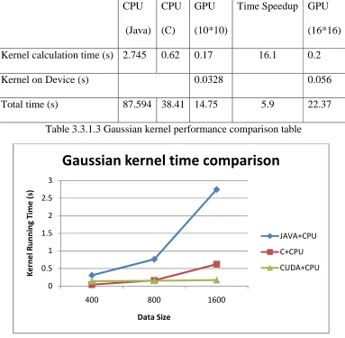
Time Speedup GPU (16*16) Kernel calculation time (s) 2.745 0.62 0.17 16.1 0.2

Total time (s) 87.594 38.41 14.75 5.9 22.37

4Table 3.3.1.3 Gaussian kernel performance comparison table

12Figure 3.3.1.1 Gaussian kernel performance comparison

0 0.5 1 1.5 2 2.5 3

400 800 1600

K e rn e l R u n n in g Ti m e ( s) Data Size

Gaussian kernel time comparison

JAVA+CPU

C+CPU

(34)

25

13Figure 3.3.1.2 SVM classification time using Gaussian kernel

From the tests above, we can see the GPU kernel calculation time is very small, which is more obvious when the dataset is larger. When the data set is small, GPU cannot show its performance advantages. The speed increases from 3 times to 16 times faster than the original java version. The total training time makes more difference -- which is 5 times faster than the original one with the data getting larger. This is because Java ,every time, needs to call the library (cern scientific matrix calculation library) then get the value, while in C there is no need to call the library. It just gets the value from the array.

3.3.2 Absdiff Kernel

For kernel functions, far away points result in large polarization values and small kernel values. We can take the other extreme. Next we consider the Absdiff kernel [21]:

BPQRSTUV W BXYZQ[[, exp \H∑ |_2O |]

400 800 1600

S V M C la ss if ic a ti o n Ti m e S p e e d U p Data Size

SVM classification time using Gaussian kernel

(35)

26 sn is: 0.920000,sp is: 0.920000,acc is: 0.920000

CPU (Java)

CPU (C)

GPU (10*10)

Time speedup GPU (16*16) Kernel calculation time (s) 0.305 0.12 0.13 2.3 0.13 Kernel on Device (s) 0.0021 0.0036 Total time (s) 2.261 0.35 0.37 6.1 0.37

5Table 3.3.2.1 Absdiff kernel performance comparison table

The performance of our C code with GPU vs Java code and C code on CPU is listed below: dataset: 9GC9TA.train, sigma: 0.5, row #: 800, column #: 150

sn is: 0.95, sp is: 0.93, acc is: 0.94

CPU (Java)

CPU (C)

GPU (10*10)

Time speedup GPU (16*16) Kernel Calculation Time (s) 0.743 0.48 0.14 5.3 0.16 Kernel on Device (s) 0.0082 0.0139 Total time (s) 5.253 2.12 1.74 3.01 1.77

The performance of our C code with GPU vs Java code and C code on CPU is listed below: dataset: 9GC9CG_9AT9TA.train, sigma: 0.5, row #: 1600, column #: 150

sn is: 0.87,sp is: 0.84,acc is: 0.855

CPU (Java)

CPU (C)

GPU (10*10)

Time speedup GPU (16*16) Kernel calculation time (s) 3.5 1.96 0.18 19.4 0.21

(36)

27

Total time (s) 64.6 17.84 11.8 5.47 12.48

14Figure 3.3.2.1 Absdiff kernel time comparison

15Figure 3.3.2.2 SVM classification time using Absdiff kernel

The performance of the Absdiff kernel is more like the Gaussian kernel, since they have almost the same number of arithmetic instructions.

0 0.5 1 1.5 2 2.5 3 3.5 4

400 800 1600

Absdiff kernel time comparison

JAVA+CPU

C+CPU

C+GPU

400 800 1600

SVM classification time using Absdiff kernel

(37)

28

3.3.3 Sentropic Kernel

Next we consider the Sentropic kernel:

B^_TVU`R, exp _O1 #a|| a||%

where

a|| a|| '

b c d

e

is the symmetric Kullback-leibler divergence.

The performance of our C code with GPU vs Java code and C code on CPU is listed below: training dataset: 9GC9TA.train, sigma: 0.5, row #: 400, column #: 150

sn is: 0.770000,sp is: 0.960000,acc is: 0.865000 CPU (Java)

CPU (C)

GPU (10*10)

Time Speedup GPU (16*16) Kernel calculation time (s) 1.12 0.787 0.14 8 0.15 Kernel on Device (s) 0.0075 0.011 Total time (s) 3.498 1.71 0.73 4.8 0.73

8Table 3.3.1.1. Sentropic kernel performance comparison table.

The performance of our C code with GPU vs Java code and C code on CPU is listed below: dataset: 9GC9TA.train, sigma: 0.5, row #: 800, column #: 150

sn is: 0.91,sp is: 0.93,acc is: 0.92

CPU (Java)

CPU (C)

GPU (10*10)

Time Speedup (s)

GPU (16*16) Kernel Calculation Time (s) 4.49 3.102 0.17 26.4 0.18

(38)

29

Total time (s) 11.44 6.08 1.81 6.4 2.32

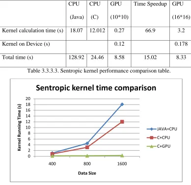
The performance of our C code with GPU vs Java code and C code on CPU is listed below: dataset: 9GC9CG_9AT9TA.train, sigma: 0.5, row: 1600, column: 150

sn is: 0.875,sp is: 0.82, acc is: 0.8475 CPU (Java) CPU (C) GPU (10*10)

Time Speedup GPU (16*16) Kernel calculation time (s) 18.07 12.012 0.27 66.9 3.2

Total time (s) 128.92 24.46 8.58 15.02 8.33

16Figure 3.3.3.1 Sentropic kernel calculation time comparison

0 2 4 6 8 10 12 14 16 18 20

400 800 1600

Sentropic kernel time comparison

JAVA+CPU

C+CPU

(39)

30

17Figure 3.3.3.2 SVM classification time using Sentropic kernel

For the Sentropic kernel, the kernel instruction is different from the first two, since we need to compare with the cutoff value before we calculate the kernel function. Therefore, most of the time gets wasted there. However, we can see that with the more function calls and the larger dataset, the C and CUDA version is more efficient than the Java version. This is true, because the function calls in C and CUDA are very light.

According to the tests above, the GPU performs faster than the CPU for the same kernel function algorithm used on different block sizes as predicted. The reason is the highly parallel architecture of the GPU. However, as we increase the block size of the GPU to 16 by 16, we notice that the performance decreases as compared to a GPU with block size 10. This occurs because in a larger block size there are more threads operating and therefore there is more context switch. In addition, although the GPU creates thread with zero overhead, the extra threads which are not used by the kernel calculation are actually still doing the comparison work by the if statement. After all, we can see that the SVM classification time has been improved

400 800 1600

SVM classification time using Sentropic kernel

(40)

31

(41)

32

Chapter 4. Chunking SVM using GPU clusters

4.1 Message Passing Interface

With all the tests above, we can see that GPU provides a cheap solution for SIMD (Single Instruction, Multiple Data) vector computation. We would like to harness this power in the scientific computation area by using GPU clusters, as we use clusters that have been built to harness the power of the standard CPU. The Message Passing Interface (MPI) helps us to combine multi-CPU and multi-GPU together.

MPI is a standard message passing library which allows a wide range of computers to communicate with each other. It has been developed and implemented by many of today’s high performance computing companies (Sun, IBM, SGI, etc.) and is mainly used for solving

significant scientific and engineering problems on parallel computers. The draft of this standard called MPI-1was presented at Supercomputing 1994. It has about 128 functions which

emphasizes message passing and has a static runtime environment. In 1998 version MPI-2.1 (called MPI-2) was completed, which includes 287 functions and adds new features like parallel I/O, dynamic process management and remote memory operations. It is important to note that 2 is mostly a superset of 1, although some functions have been deprecated. Thus MPI-1.2 programs still work under MPI implementations compliant with the MPI-2 standard.

(42)

The paradigm of an MPI program can be understoo responsible for decomposing the problem into

slaves process, and gathers the partial results in order to produce the final computation; 2) the slave nodes execute in

task, process the task, and send

18Figure 3.4.1 MPI data sending construction model

4.2 Combine MPI and

If the MPI implementation

show a response for a larger parallel part machines, while within each, CUDA

There are some similarities

MPI_Comm_rank() are constant variab

know to create the number of parallel threads to run within a thread the number of machines that user defined to

increasing values from 0 to the number that user defined. synchronization mechanisms for the

return the correct value for each round

33

MPI program can be understood in two parts: 1) the m ecomposing the problem into small tasks and distributes these

the partial results in order to produce the final result of the slave nodes execute in very simple cycles which get the m

and send the results to the master (see figure 3.4.1).

Figure 3.4.1 MPI data sending construction model

PI and CUDA

MPI implementation is compared to the CUDA one, the MPI implementation should parallel part, which means that MPI distributes

CUDA is used to do its smaller parallel part of between these two in implementing parallel task. are constant variable. threadIdx can be initialized by the user

the number of parallel threads to run within a thread block. MPI_Comm_rank() is that user defined to parallel running among the cluster.

from 0 to the number that user defined. They both have the similar for the all of the threads to finish each round of parallel work return the correct value for each round: syncthreads() vs MPI_Barrier().

the master node is small tasks and distributes these tasks to a farm of

result of the

the message with the

Figure 3.4.1 MPI data sending construction model

, the MPI implementation should s work to all of the part of work.

in implementing parallel task. threadIdx vs the user to let the GPU block. MPI_Comm_rank() is among the cluster. They are self- They both have the similar

(43)

34

There are some differences between the two as well. CUDA uses shared memory for all of the threads within the same block to communicate with each other. All of the threads can be

synchronized only within the thread block. The communication within the shared memory and transferring data from global memory to shared memory is very cheap compared with the data transformation between machines using MPI, which is highly dependent on network latency.

We have run our SVM chunking algorithm on four machines. We put our dataset (1600 by 150 dimensions) on a network shared hard disk and each machine will read one chunk of this dataset to send it to the GPU to calculate kernel function then start to run SVM within this chunk. After each chunk converges, the result will be send back to the master machine. In order to avoid wasting time on transferring data back and forth, we only use MPI to send the indexes of the resulting dataset and re-chunk the data using the changed indexes, then continue to run kernel function on GPU and finally run SVM on all of the machines. This step will stop unless the merged data chunk is smaller than twice the size of the first chunk layer (see figure3.5.1 for data sending structure).

(44)

19Figure 3.5.1 Combine MPI and CUDA data sending model

35

(45)

36

20Figure 3.5.2 MPI-CUDA flowchart

4.3 Results

Clusters’ environment: 4 Ubuntu machines: each of them has 4 processors and each processor is Intel Core 2 Extreme CPU Q6850 3.00GHz. Memory is 2GB. GPU is NVIDIA Corporation GeForce 8800 Ultra and has two on each machine.

We decided to use the Absdiff kernel, since after testing the three kernels, Absdiff was chosen as the best kernel for the DNA hairpin datasets because of its high accuracy (average is: 90.5) and because it takes the least amount of time to converge. The training dataset is

(46)

37

(47)

38

Chapter 5. Conclusion

SVM is a very useful technique in the area of classification. It has been utilized in various pattern recognition applications. However, a main constraint of SVM is its training time often costing a lot of time when a large dataset is being classified. Then the very natural way to solve this problem is using data parallelism to break the data into many small chunks. After obtaining results from these small chunks, we can trace back the original problem and then make it easier to solve.

GPU is very popular now in scientific computation domains. Because of its highly paralleled architecture, we can implement SVM on GPU which can help improve the performance on SVM classification time. Although GPU has a lot of limitations, such as shared memory is very small and only one kernel function can be execute on one GPU card at one time, we can also

implement our SVM on it, as long as we manage the memory carefully. As shown in table 3.3 serial, we conclude that GPU can improve SVM performance a lot better than CPU while maintaining the same accuracy as C and Java.

Although the testing result on distributed machine with many GPUs is not well illustrated, we still have space to improve it. For example, the SVM kernel function part on GPU needs to be revised to take the thread block size not only as a squared number but as any number.

With the chunking idea, the problem of a larger dataset running on SVM would not be a problem anymore and several machines could be utilized together to make the classification process faster. In addition, for reaching the highest level of performance, in the future, multiple GPUs could be used as one time; in this case we could have distributed machines with

(48)

39

References

[1] B. E. Boser, I. Guyon, V. Vapnik: A Training Algorithm for Optimal Margin Classifiers. Proceedings of the Fifth Annual Workshop on Computational Learning Theory 144-152, 1992. [2] J.C. Platt: Sequential Minimal Optimization: A Fast Algorithm for Training Support Vector Machines, Microsoft Research, Technical Report MSR-TR-98-14, 1998.

[3] E. Osuna, R. Freund, F. Girosi: Improved Training Algorithm for Support Vector Machines," Proc. IEEE NNSP ’97, 1997.

[4] Handwriting recognition: Wikipedia.

[5] C. Bahlmann, B. Haasdonk , H. Burkhardt : On-line Handwriting Recognition with Support Vector Machines—A Kernel Approach, publ. in Proc. of the 8th Int. Workshop on Frontiers in Handwriting Recognition (IWFHR), pp. 49–54, 2002.

[6] A. Ganapathiraju, J. E. Hamaker, J. Picone: Applications of Support Vector Machines to Speech Recognition, IEEE Transactions on Signal Processing; Vol. 52 Issue 8, Aug2004. [7] L. Bottou et al. Comparison of classifier methods: a case study in handwritten digit

recognition. Proceedings of the 12th IAPR International Conference on Pattern Recognition, vol. 2, pp. 77-82.

[8] C.J. C. Burges: A tutorial on support vector machines for pattern recognition, Knowledge Discovery Data Mining, vol. 2, no. 2, pp. 121–167, 1998.

[9] V. N. Vapnik: Statistical Learning Theory. New York: Wiley, 1998.

[10] J. Padrell-Sendra, D. Mart´ın-Iglesias and F. D´ıaz-de-Mar´ıa: Support Vector Machines for Continuous Speech Recognition

(49)

40

[12] S. Winters-Hilt, A. Davis, I. Amin, E. Morales: Nanopore current transduction analysis of protein binding to non-terminal and terminal DNA regions: analysis of transcription factor binding, retroviral DNA terminus dynamics, and retroviral integrase-DNA binding, BMC Bioinformatics, 2007

[13] H.P., Graf, E., Cosatto, L., Bottou, I., Durdanovic, V., Vapnik: Parallel Support Vector Machines: The Cascade SVM, in proceedings NIPS, 2004

[14] S. Winters-Hilt, and K. Armond Jr.: Distributed SVM Learning and Support Vector Reduction, Department of Computer Science, University of New Orleans

[15] J. Mercer: Functions of positive and negative type and their connection with the theory of integral equations, Philos. Trans. Roy. Soc. London 1909

[16] Sam Meren, thesis 2008

[17] S. Winters-Hilt, E. Morales, I. Amin, and A. Stoyanov: Nanopore-based kinetics analysis of individual antibody-channel and antibody-antigen interactions, 8(Suppl 7): S20, BMC

Bioinformatics, 2007

[18] W. Gropp, E. Lusk and A. Skjellum: “Using MPI: portable parallel programming with the message-passing interface”. MIT Press In Scientific And Engineering Computation Series, Cambridge, MA, USA. 307 pp, 1994

[19] video: http://www.youtube.com/watch?v=nlGnKPpOpbE [20] NVIDIA CUDA programming guide 2.0

(50)

41

Appendix

A1.C++ code implement SVM

/* * SVM.c *

* Created on: Feb 5, 2009 * Author: Hang Zhang */

#include "SVM.h"

SVMModel *learnSVM(SVMModel *model,dataoutput *dataoutputInst, const int RowNum, const int ColNum,float parameter2, int type, int argc, char** argv) {

printf("training... row=%d, col=%d \n",RowNum,ColNum); float* inputFeatures = dataoutputInst->inputFeatures1d; float* inputLabels = dataoutputInst->inputLabels;

clock_t kerneltime=clock();

float* kernelMat=kernelMatrix(inputFeatures,inputFeatures,RowNum,ColNum,RowNum,sigma, type, argc, argv); printf("\nsvm kernel time is:%f, ",((double)clock()-kerneltime));

float *alpha=new float[RowNum]; float *errorCache=new float[RowNum]; float threshold=0;

int numChanged; int examineAll; int i;

int supp = 0;

/* Initialize alpha array to all zero */ for (i = 0; i < RowNum; i++) {

alpha[i] = 0; errorCache[i] = 0; }

numChanged = 0; examineAll = 1; int iter=0; int maxIter=1000; clock_t start,finish;//time float costtime;

start = clock();

while ((numChanged > 0 || examineAll == 1) && iter < ((maxIter == 0)?iter+1:maxIter)) { iter++;

numChanged = 0; if (examineAll == 1) {

/* Loop over all training examples */ for (i = 0; i < RowNum; i++) {

numChanged += examineExample(i,inputLabels,RowNum,kernelMat,&threshold,alpha, errorCache);

}

// printf("examineAll=1\n"); } else {

/* Loop over examples where alpha is not 0 & not C */ for (i = 0; i < RowNum; i++)

if (alpha[i] != 0 && alpha[i] != cVal) { numChanged +=

examineExample(i,inputLabels,RowNum,kernelMat,&threshold,alpha, errorCache); }

}

(51)

42

examineAll = 0; else if (numChanged == 0)

examineAll = 1; }

finish = clock(); costtime = finish-start;

printf("\ntraining time spend (ms): %f, iteration: %d, threshold: %f", costtime, iter, threshold); delete(errorCache);

//*****************construct SVM Model*****************

{

model->setIter=iter;

model->setThreshold=threshold; vector<int> nonZeroAlphaIndList; vector<int> polarizationIndList;

int upto = 0;

for (int i = 0; i < RowNum; i++) { float thisalpha = alpha[i];

if (thisalpha > 0 && thisalpha != cVal){ nonZeroAlphaIndList.push_back(i); }

// count the vectors in the polarization set if (thisalpha == 0) {

polarizationIndList.push_back(i); }

++upto; } /*

* allocate the alpha corresponding to support vectors */

float* tmpSvAlphas = new float[nonZeroAlphaIndList.size()]; for (int i = 0; i < (int)nonZeroAlphaIndList.size(); i++) {

tmpSvAlphas[i]= alpha[nonZeroAlphaIndList.at(i)]; }

model->setSvAlphas=tmpSvAlphas;///

model->setsupp=(int)nonZeroAlphaIndList.size(); /////

int suppLength=(int)nonZeroAlphaIndList.size(); int nonSuppLength=(int)polarizationIndList.size();

int* nonZeroAlphaIndArray=new int[nonZeroAlphaIndList.size()]; int* polarizationIndArray=new int[polarizationIndList.size()];

for(int i=0; i<suppLength;i++){

nonZeroAlphaIndArray[i]=nonZeroAlphaIndList.at(i); } model->setSvIndices=nonZeroAlphaIndArray;//// for(int i=0;i<nonSuppLength;i++){ polarizationIndArray[i]=polarizationIndList.at(i); }

model->setPolarizationIndices=polarizationIndArray; ////

//allocate original features

model->setSuppFeatures=viewSelectionFeats(inputFeatures,nonZeroAlphaIndArray,suppLength, ColNum); // allocate original labels

model->setSvLabels=viewSelectionLabel(inputLabels, nonZeroAlphaIndArray,suppLength); printf("\n #SV = %d, threshold = %f, Iterations: %d", nonZeroAlphaIndList.size(), model->setThreshold, iter);

(52)

43

free(kernelMat); return model; }

float* viewSelectionFeats(float* feats,int* thisIndex, int thisLength, int ColNum){ unsigned int size_features = thisLength*ColNum;

unsigned int mem_size_features= sizeof(float) * size_features; float* selectFinal = (float*) malloc(mem_size_features); for(int i=0;i<thisLength;i++){ for(int j=0;j<ColNum;j++) selectFinal[i*ColNum+j]=feats[(thisIndex[i])*ColNum+j]; } return selectFinal; }

float* viewSelectionLabel(float* labels,int* thisIndex, int thisLength){ float* selectFinal=new float[thisLength];

for(int i=0;i<thisLength;i++){

selectFinal[i]=labels[(thisIndex[i])]; }

return selectFinal; }

float outputNonlinear(int i,float *inputLabels,const int RowNum, float *kernelMat, float *threshold,float *alpha) {

float alphaJ = 0; float sum = 0;

for (int j=0; j < RowNum; j++){ if ((alphaJ = alpha[j]) > 0){

sum += alphaJ * inputLabels[j] *kernelMat[i*RowNum+j]; }

}

return sum - *threshold; }

int examineExample(int i2,float *inputLabels, const int RowNum, float *kernelMat, float *threshold, float *alpha, float *errorCache) {

float r2=0; float E2=0;

float alph2 = alpha[i2]; float y2 = inputLabels[i2]; float tol=tolerance;

if (alph2 > 0 && alph2 < cVal) E2 = errorCache[i2]; else

E2 = outputNonlinear(i2,inputLabels,RowNum, kernelMat, threshold, alpha) - y2;

r2 = E2 * y2;

/*

* if alpha2 violates the KKT condition within a tolerance

* then look for an alpha1 and optimize both alphas (take_step(i1,i2)) */

if ((r2 < -tol && alph2 < cVal) || (r2 > tol && alph2 > 0)) {

{

/*

(53)

44

*/ int i1 = -1; float tmax = 0;

for (int k = 0; k < RowNum; k++) {

float alpha_k = alpha[k];

if (0 < alpha_k && alpha_k < cVal) {

float temp;

float E1 = errorCache[k];

/*

* SMO approximates the step size by absolute value of (E1-E2) */

temp = abs(E1 - E2); if (temp > tmax) {

tmax = temp; i1 = k; }

} }

if (i1 > -1 )

if (takeStep(i1, i2,RowNum, inputLabels,kernelMat,threshold, alpha, errorCache) == 1) return 1;

}

/*

* At this point no positive progress was made (last paragraph * in Platt's paper section 2.4).

*

* first check the non bound alphas from a random place */

{ srand(0); int k = 0; int i1 = -1;

// int k0 = abs(rand()*327688*RowNum); int k0 = abs(rand()*RowNum);

for (k = k0; k < RowNum + k0; k++) {

i1 = k % RowNum; float alpha_k = alpha[i1];

if (0 < alpha_k && alpha_k < cVal) {

if (takeStep(i1, i2,RowNum, inputLabels,kernelMat, threshold, alpha, errorCache)== 1) return 1; } } } /*

* if still no progress then iterate through all feature vectors * starting from a random place

*/

{ srand(0);

int k = 0, i1=-1;

// int k0 = abs(rand()*327688*RowNum); int k0 = abs(rand()*RowNum);

(54)

45

{

i1 = k % RowNum;

if (takeStep(i1, i2,RowNum,inputLabels,kernelMat,threshold,alpha,errorCache) == 1) return 1; } } } return 0; }

int takeStep(int i1, int i2, const int RowNum, float *inputLabels, float *kernelMat, float *threshold, float *alpha, float *errorCache) {

float eps=epsilon;

float alpha_old_1, alpha_old_2; // old_values of alpha_1, alpha_2 float alpha_new_1, alpha_new_2; // new values of alpha_1, alpha_2 float y1, y2, s, E1, E2, L, H, k11, k22, k12, eta, Lobj, Hobj;

if (i1 == i2) return 0;

alpha_old_1 = alpha[i1]; y1 = inputLabels[i1];

if (alpha_old_1 > 0 && alpha_old_1 < cVal) E1 = errorCache[i1];

else

E1 = outputNonlinear(i1,inputLabels,RowNum, kernelMat,threshold, alpha) - y1;

alpha_old_2 = alpha[i2]; y2 = inputLabels[i2];

if (alpha_old_2 > 0 && alpha_old_2 < cVal) E2 = errorCache[i2];

else

E2 = outputNonlinear(i2,inputLabels,RowNum,kernelMat,threshold, alpha) - y2;

s = y1 * y2;

if (y1 == y2) {

float gamma = alpha_old_1 + alpha_old_2; if (gamma > cVal)

{

L = gamma-cVal; H = cVal; }

else {

L = 0; H = gamma; }

} else {

float gamma = alpha_old_2 - alpha_old_1; if (gamma > 0)

{

L = gamma; H = cVal; }

(55)

46

{

L = 0;

H = cVal + gamma; }

}

if (L == H){ return 0; }

k11=kernelMat[i1*RowNum+i1]; k12=kernelMat[i1*RowNum+i2]; k22=kernelMat[i2*RowNum+i2];

eta = k11 + k22 - 2*k12;

if (eta > 0) {

alpha_new_2 = alpha_old_2 + y2 * (E1 - E2) / eta; if (alpha_new_2 < L)

alpha_new_2 = L; else if (alpha_new_2 > H)

alpha_new_2 = H; }

else {

float f1 = y1 * (E1 + *threshold) - alpha_old_1 * k11 - s * alpha_old_2 * k12; float f2 = y2 * (E2 + *threshold) - alpha_old_2 * k22 - s * alpha_old_1 * k12; float l1 = alpha_old_1 + s * (alpha_old_2-L);

float h1 = alpha_old_1 + s * (alpha_old_2-H);

Lobj = l1*f1 + L*f2 + 1/2 * ( (l1*l1)*k11 + (L*L)*k22 + 2*s*L*l1*k12 ); Hobj = h1*f1 + H*f2 + 1/2 * ( (h1*h1)*k11 + (H*H)*k22 + 2*s*H*h1*k12 );

if (Lobj < Hobj-eps) alpha_new_2 = L; else if (Lobj > Hobj+eps)

alpha_new_2 = H; else

alpha_new_2 = alpha_old_2;

}

if (abs(alpha_new_2 - alpha_old_2)< eps * (alpha_new_2 + alpha_old_2 + eps) ) return 0;

alpha_new_1 = alpha_old_1 + s * (alpha_old_2 - alpha_new_2);

if (alpha_new_1 < 0) {

alpha_new_2 += s * alpha_new_1; alpha_new_1 = 0;

}

else if (alpha_new_1 > cVal) {

float t = alpha_new_1 - cVal; alpha_new_2 += s * t; alpha_new_1 = cVal; }

/* updating the threshold */ float b1, b2, bnew, delta_b;

(56)

47

b2 = *threshold + E2 + y1 * (alpha_new_1 - alpha_old_1) * k12 + y2 * (alpha_new_2 - alpha_old_2) * k22;

if (alpha_new_1 > 0 && alpha_new_1 < cVal) bnew = b1;

else if (alpha_new_2 > 0 && alpha_new_2 < cVal) bnew = b2;

else

bnew = (b1 + b2) / 2;

delta_b = bnew - *threshold; *threshold = bnew;

/*

* updating the error cache */

float t1 = y1 * (alpha_new_1-alpha_old_1); float t2 = y2 * (alpha_new_2-alpha_old_2);

for (int i = 0; i < RowNum; i++) {

float alpha_i = alpha[i];

if (0 < alpha_i && alpha_i < cVal) {

float k1i=kernelMat[i1*RowNum+i]; float k2i=kernelMat[i2*RowNum+i];

float error_old_i = errorCache[i];

float error_new_i = error_old_i + t1*k1i + t2*k2i - delta_b; errorCache[i]=error_new_i; } } errorCache[i1]= 0; errorCache[i2]= 0; /*

* updating the alphas */

alpha[i1]= alpha_new_1; alpha[i2]= alpha_new_2;

return 1; }

A2. Host code to launch the GPU function call

SVM_kernel_host.cu

// includes, kernels

#include "Absdiff_kernel_device.cu"

#include "Gaussian_kernel_device.cu"

#include "Sentropic_kernel_device.cu"

// includes, project #include <cutil_inline.h>

(57)

48

void printDiff(float*, float*, int, int); void printAB(float*, float*, int , int);

void AbsdiffGold( float*, const float*, const float*, unsigned int, unsigned int,unsigned int, float); void GaussianGold( float*, const float*, const float*, unsigned int, unsigned int,unsigned int, float); void SentropicGold( float*, const float*, const float*, unsigned int, unsigned int,unsigned int, float);

////////////////////////////////////////////////////////////////////////////////////

float* kernelMatrix(float* features1, float* features2, int RowNum, int ColNum, int RowNum2,float sigma, int type, int argc, char** argv){

if( cutCheckCmdLineFlag(argc, (const char**)argv, "device") ) cutilDeviceInit(argc, argv);

else

cudaSetDevice( cutGetMaxGflopsDeviceId() ); float parameter =1/(2*sigma*sigma);

float parameter2=1/(sigma*sigma);

// allocate host memory for matrices A and B unsigned int size_A = RowNum * ColNum; unsigned int mem_size_A = sizeof(float) * size_A;

unsigned int size_B = RowNum2 * ColNum; unsigned int mem_size_B = sizeof(float) * size_B;

float* d_A;

cutilSafeCall(cudaMalloc((void**) &d_A, mem_size_A)); float* d_B;

cutilSafeCall(cudaMalloc((void**) &d_B, mem_size_B));

// copy host memory to device

cutilSafeCall(cudaMemcpy(d_A, features1, mem_size_A, cudaMemcpyHostToDevice) ); cutilSafeCall(cudaMemcpy(d_B, features2, mem_size_B, cudaMemcpyHostToDevice) );

// allocate device memory for result

unsigned int size_C = RowNum * RowNum2; unsigned int mem_size_C = sizeof(float) * size_C; float* d_C;

cutilSafeCall(cudaMalloc((void**) &d_C, mem_size_C));

// allocate host memory for the result float* h_C = (float*) malloc(mem_size_C);

// create and start timer unsigned int timer = 0;

cutilCheckError(cutCreateTimer(&timer)); cutilCheckError(cutStartTimer(timer));

// setup execution parameters

dim3 threads(BLOCK_SIZE, BLOCK_SIZE);

dim3 grid(RowNum2 / threads.x, RowNum / threads.y); // execute the kernel

switch(type){

case 0: AbsdiffKernel<<< grid, threads >>>(d_C, d_A, d_B, RowNum, ColNum, parameter); break; case 1: GaussianKernel<<< grid, threads >>>(d_C, d_A, d_B, RowNum, ColNum, parameter); break; case 2: SentropicKernel<<< grid, threads >>>(d_C, d_A, d_B, RowNum, ColNum, parameter2); break; }

// check if kernel execution generated and error cutilCheckMsg("Kernel execution failed");

(58)

49

cutilCheckError(cutStopTimer(timer));

printf("kernel on the device Processing time: %f (ms) \n", cutGetTimerValue(timer)); cutilCheckError(cutDeleteTimer(timer));

// copy result from device to host

cutilSafeCall(cudaMemcpy(h_C, d_C, mem_size_C, cudaMemcpyDeviceToHost) );

cutilSafeCall(cudaFree(d_A)); cutilSafeCall(cudaFree(d_B)); cutilSafeCall(cudaFree(d_C)); cudaThreadExit(); return h_C; }

A3. Absdiff kernel function code on GPU, BLOCKSIZE=10 Absdiff_kernel_device.cu

/*

* Device code. */

#ifndef _ABSDIFF_KERNEL_DEVICE_H_ #define _ABSDIFF_KERNEL_DEVICE_H_

#include <stdio.h>

#include "SVM_kernel_host.h"

#define CHECK_BANK_CONFLICTS 0 #if CHECK_BANK_CONFLICTS

#define AS(i, j) cutilBankChecker(((float*)&As[0][0]), (BLOCK_SIZE * i + j)) #define BS(i, j) cutilBankChecker(((float*)&Bs[0][0]), (BLOCK_SIZE * i + j)) #else

#define AS(i, j) As[i][j] #define BS(i, j) Bs[i][j] #endif

////////////////////////////////////////////////////////////////////////// //absdiff kernel

////////////////////////////////////////////////////////////////////////// __global__ void

AbsdiffKernel( float* C, float* A, float* B, int RowNum, int ColNum, float Para) {

// Block index int bx = blockIdx.x; int by = blockIdx.y;

// Thread index int tx = threadIdx.x; int ty = threadIdx.y;

// Index of the first sub-matrix of A processed by the block int aBegin = ColNum * BLOCK_SIZE * by;

// Index of the last sub-matrix of A processed by the block int aEnd = aBegin + ColNum - 1;

// Step size used to iterate through the sub-matrices of A int aStep = BLOCK_SIZE;

(59)

50

int bBegin = ColNum * BLOCK_SIZE * bx;

// Step size used to iterate through the sub-matrices of B int bStep = BLOCK_SIZE;

// Csub is used to store the element of the block sub-matrix // that is computed by the thread

float Csub = 0; float Cresult=0;

// Loop over all the sub-matrices of A and B // required to compute the block sub-matrix for (int a = aBegin, b = bBegin;

a <= aEnd;

a += aStep, b += bStep) {

// Declaration of the shared memory array As used to // store the sub-matrix of A

__shared__ float As[BLOCK_SIZE][BLOCK_SIZE];

// Declaration of the shared memory array Bs used to // store the sub-matrix of B

__shared__ float Bs[BLOCK_SIZE][BLOCK_SIZE];

// Load the matrices from device memory // to shared memory; each thread loads // one element of each matrix AS(ty, tx) = A[a + ColNum * ty + tx]; BS(ty, tx) = B[b + ColNum * ty + tx];

// Synchronize to make sure the matrices are loaded __syncthreads();

// Calculate the two matrices together; // each thread computes one element // of the block sub-matrix

for (int k = 0; k < BLOCK_SIZE; ++k){ Csub += abs(BS(tx, k)-AS(ty,k)); }

__syncthreads(); }

// Write the block sub-matrix to device memory; // each thread writes one element

float norm1_diff_squared = sqrtf(Csub); Cresult=expf(-Para*norm1_diff_squared); int Row=by*BLOCK_SIZE+ty;

int Row2=bx*BLOCK_SIZE+tx;

C[RowNum * Row + Row2] = Cresult; }

#endif // #ifndef _ABSDIFF_KERNEL_H_

A4. Absdiff kernel function code on GPU, BLOCK_SIZE=16 Absdiff_kernel_device.cu

/*

(60)

51

#ifndef _ABSDIFF_KERNEL_DEVICE_H_ #define _ABSDIFF_KERNEL_DEVICE_H_

#include <stdio.h>

////////////////////////////////////////////////////////////////////////// //absdiff kernel

////////////////////////////////////////////////////////////////////////// __global__ void

AbsdiffKernel( float* C, float* A, float* B, int RowNum, int ColNum, float Para) {

// Block index int bx = blockIdx.x; int by = blockIdx.y;

// Thread index int tx = threadIdx.x; int ty = threadIdx.y;

// Index of the first sub-matrix of A processed by the block int aBegin = ColNum * BLOCK_SIZE * by;

// Index of the last sub-matrix of A processed by the block int aEnd = aBegin + ColNum - 1;

// Step size used to iterate through the sub-matrices of A int aStep = BLOCK_SIZE;

// Index of the first sub-matrix of B processed by the block int bBegin = ColNum * BLOCK_SIZE * bx;

// Step size used to iterate through the sub-matrices of B int bStep = BLOCK_SIZE;

int remainderA=ColNum % BLOCK_SIZE;

// Csub is used to store the element of the block sub-matrix // that is computed by the thread

float Csub = 0; float Cresult=0;

// Loop over all the sub-matrices of A and B // required to compute the block sub-matrix for (int a = aBegin, b = bBegin;

a <= aEnd;

a += aStep, b += bStep) {

__shared__ float As[BLOCK_SIZE][BLOCK_SIZE];

__shared__ float Bs[BLOCK_SIZE][BLOCK_SIZE];

if (a==aBegin+(ColNum/BLOCK_SIZE)*BLOCK_SIZE){ if(tx<remainderA){

AS(ty, tx) = A[a + ColNum * ty + tx]; BS(ty, tx) = B[b + ColNum * ty + tx]; }

(61)

52

for (int k = 0; k < remainderA; ++k){ Csub += abs(BS(tx, k)-AS(ty,k)); }

__syncthreads(); }else {

AS(ty, tx) = A[a + ColNum * ty + tx]; BS(ty, tx) = B[b + ColNum * ty + tx]; __syncthreads();

for (int k = 0; k < BLOCK_SIZE; ++k){ Csub += abs(BS(tx, k)-AS(ty,k)); }

__syncthreads(); }

}

float norm1_diff_squared = sqrtf(Csub); Cresult=expf(-Para*norm1_diff_squared); int Row=by*BLOCK_SIZE+ty;

int Row2=bx*BLOCK_SIZE+tx;

C[RowNum * Row + Row2] = Cresult; }

#endif // #ifndef _ABSDIFF_KERNEL_H_

A5. Gaussian kernel function code on GPU, BLOCK_SIZE=10 Gaussian_kernel_device.cu

/*

* Device code. */

#ifndef _GAUSSIAN_KERNEL_DEVICE_H_ #define _GAUSSIAN_KERNEL_DEVICE_H_

#include <stdio.h>

////////////////////////////////////////////////////////////////////////// //absdiff kernel

////////////////////////////////////////////////////////////////////////// __global__ void

GaussianKernel( float* C, float* A, float* B, int RowNum, int ColNum, float Para) {

int bx = blockIdx.x; int by = blockIdx.y;

int tx = threadIdx.x; int ty = threadIdx.y;

int aBegin = ColNum * BLOCK_SIZE * by;

Distributed Support Vector Machine With Graphics Processing Units

ScholarWorks@UNO

ScholarWorks@UNO

Distributed Support Vector Machine With Graphics Processing

Distributed Support Vector Machine With Graphics Processing

Units

Units

Acknowledgments

Table of Contents

List of Figures

List of Tables

List of Illustrations

Abstract

Keywords

Chapter 1. Introduction

1.1 Motivation

1.2 Overview

Chapter 2. Support Vector Machines

2.1Introduction

2.2 SVM Applications

2.3 Find the Decision Hyperplane

2.4 Kernel Functions

2.5 Mercer’s conditions

2.6 Dataset Acquisition

2.7 SVM Chunking Methods

Chapter 3. Implementation of Chunking SVM with GPU

3.1 Introduction to GPU

3.2 CUDA Programming

NVIDIA developed an architecture which is for general purpose parallel computing called

3.3 SVM Kernel Implementations on GPU

3.3.1 Gaussian Kernel

Gaussian kernel time comparison

3.3.2 Absdiff Kernel

SVM classification time using Gaussian kernel

Absdiff kernel time comparison

SVM classification time using Absdiff kernel

3.3.3 Sentropic Kernel

Sentropic kernel time comparison

SVM classification time using Sentropic kernel

Chapter 4. Chunking SVM using GPU clusters

4.1 Message Passing Interface

4.2 Combine MPI and

PI and CUDA

4.3 Results

Chapter 5. Conclusion

References

Appendix