Sinc operational matrix method for solving the Bagley-Torvik
equa-tion
Mohammad-Reza Azizi∗
Department of Mathematics, Faculty of Sciences, Azarbaijan Shahid Madani University, Tabriz, Iran. E-mail: [email protected]
Ali Khani
Department of Mathematics, Faculty of Sciences, Azarbaijan Shahid Madani University, Tabriz, Iran. E-mail: [email protected]
Abstract The aim of this paper is to present a new numerical method for solving the Bagley-Torvik equation. This equation has an important role in fractional calculus. The fractional derivatives are described based on the Caputo sense. Some properties of the sinc functions required for our subsequent development are given and are utilized to reduce the computation of solution of the Bagley-Torvik equation to some algebraic equations. It is well known that the sinc procedure converges to the solution at an exponential rate. Numerical examples are included to demonstrate the validity and applicability of the technique.
Keywords. Bagley-Torvik equation, Sinc functions, Operational matrix, Caputo derivative, Numerical
methods.
2010 Mathematics Subject Classification. 65L60, 26A33.
1. Introduction
A history of fractional calculus, i.e. the theory of derivatives and integrals of frac-tional (non-integer) order, can be found in [11, 14, 16]. Both differential equations and fractional differential equations have been used to model physical and engineering processes such as electromagnetic, acoustics, viscoelasticity, electroanalytical chem-istry, neuron modeling, diffusion processing and material sciences (see for example [2, 5, 7, 13, 20] and the references therein). The analytic results on existence and uniqueness of solutions to fractional differential equations have been investigated by many authors [7, 16]. In general, most of the fractional differential equations do not have exact solutions. Recently increased attention has turned to comparing numeri-cal methods for solving fractional differential equations, fractional partial differential equations, fractional integro-differential equations and dynamic system containing fractional derivative (see for example [3,8,12,18,21,22,23]).
Received: 13 January 2017 ; Accepted: 1 March 2017.
∗Corresponding author.
In this study, we consider the Bagley-Torvik equation
A1y(2)+A2y(3/2)+A3y=f(x), x∈[0,1], (1.1)
with the boundary conditions
y(0) =a, y(1) =b, (1.2)
whereA1, A2, A3, a, bare real constants andy(x) is an unknown function. The
Bagley-Torvik equation arises in modeling of the motion of a thin rigid plate immersed in a Newtonian fluid [6, 16]. This equation has been numericaly solved by using the hybridizable discontinuous Galerkin methods [6], pseudo-spectral scheme [3], Bessel collocation method [28], generalized Taylor collocation method [1], Haar wavelet, [17] and hybrid functions [10].
In the present paper we intend to extend the application of sinc mthods to solve the Bagley-Torvik equation. Sinc function properties are discussed thoroughly in [9,26] and it is widely used for solving a wide range of problems arising from scientific and en-gineering applications including Hallen’s integral equation [25], third-order boundary value problems [24], squeezing flow [19], fractional convection-diffusion equations [23], differential-algebraic equations [27] and Thomas-Fermi equation [15].
Our method consists of reducing the problem to the solution of algebraic equations by expanding the required approximate solution as the elements of the sinc func-tions with unknown coefficients. The properties of sinc funcfunc-tions are then utilized to evaluate the unknown coefficients.
The organization of the rest of this paper is as follows: In Section 2, we introduce some necessary definitions and mathematical preliminaries of sinc functions, fractional calculus and Gauss-Jacobi quadrature. In Section 3, the new method proposed in the current work is presented. As a result a set of algebraic equations is formed and a solution of the considered problem is introduced. In Section 4, several numerical results are given to show the efficiency of our methods. In Section 5, we give a brief conclusion.
2. Preliminaries and notations
2.1. A short overview on sinc functions.
The goal of this section is to recall properties and definition of the sinc function. These are discussed thoroughly in [9,26]. The sinc function is defined on the whole real line,−∞< x <∞, by
sinc(x) =
{ sin(πx)
πx , x̸= 0,
1, x= 0.
Forh > 0, andk = 0,±1,±2, . . ., the translated sinc functions with evenly spaced nodes are given by
S(k, h)(x) = sinc
(
x−kh h
)
=
{sin[π h(x−kh)] π
h(x−kh)
, x̸=kh,
The sinc function for the interpolating pointsxj=jhis given by
S(k, h)(jh) =δkj=
{
1, k=j, 0, k̸=j.
If a functionf(x) is defined on the real axis, then forh >0 the series
C(f, h)(x) =
∞ ∑
k=−∞
f(kh) Sinc
(
x−kh h
)
,
is called the Whittaker cardinal expansion off whenever this series converges. The properties of Whittaker cardinal expansion have been extensively studied in [9]. These properties are derived in the infinite stripDS of the complexw-plane, where ford >0,
DS =
{
w=t+is :|s|< d≤π 2
}
.
Approximations can be constructed for infinite, semi-infinite and finite intervals. To construct approximations on the interval (0,1), which is used in this paper, the eye-shaped domain in the z-plane
DE=
{
z=x+iy :arg
(
z 1−z
)
< d≤π 2
}
,
is mapped conformally onto the infinite stripDS via
w=ϕ(z) = ln
(
z 1−z
)
.
The basis functions on (0,1) are taken to be the composite translated sinc functions,
Sk(x) =S(k, h)◦ϕ(x) = sinc
(
ϕ(x)−kh h
)
, (2.2)
whereS(k, h)◦ϕ(x) is defined byS(k, h)(ϕ(x)). The inverse map ofw=ϕ(z) is
z=ϕ−1(w) = exp(w) 1 + exp(w).
Thus we may define the inverse images of the real line and of the evenly spaced nodes {kh}∞k=−∞ as
Γ ={ψ(t)∈DE :−∞< t <∞}= (0,1), and
xk =ϕ−1(kh) = e kh
1 +ekh , k= 0,±1,±2, . . . (2.3) respectively.
The class of functions such that the known exponential error estimates exist for sinc interpolation is denoted byB(DE) and is defined in the following.
Definition 2.1. LetB(DE) be the class of functionsF which are analytic inDE,
satisfy ∫
ψ(t+L)
whereL={iv :|v|< d≤ π2}, and on the boundary ofDE, (denoted∂DE), satisfy
N(F) =
∫
∂DE
|F(z)dz|<∞.
Interpolation for function in B(DE) are defined in the following theorem whose proof can be found in [26].
Theorem 2.2. If ϕ′F ∈B(DE) then for allx∈Γ
F(x)−
∞ ∑
k=−∞
F(xk)S(k, h)◦ϕ(x)
≤
N(F ϕ′) 2πdsinh(πd/h)
≤2N(F ϕ′) πd e
−πd/h.
Moreover, if|F(x)| ≤Ce−α|ϕ(x)|, x∈Γ,for some positive constantsC andα, and if
the selectionh=√πd/αN≤2πd/ln 2, then
F(x)−
N
∑
k=−N
F(xk)S(k, h)◦ϕ(x)
≤C2
√
Nexp(−√πdαN), x∈Γ,
whereC2 depends only onF, dandα.
The above expressions show sinc interpolation onB(DE) converge exponentially [26]. We also require derivatives of composite sinc functions evaluated at the nodes. The expressions required for the present discussion are [23].
δk,j(0) = [S(k, h)◦ϕ(x)]|x=xj = {
1, k=j,
0, k̸=j. (2.4)
δk,j(1) = h d
dϕ[S(k, h)◦ϕ(x)]|x=xj = {
0, k=j,
(−1)j−k
j−k , k̸=j.
(2.5)
δk,j(2) = h2 d
2
dϕ2[S(k, h)◦ϕ(x)]|x=xj = {−π2
3 , k=j,
−2(−1)j−k
(j−k)2 . k̸=j.
(2.6)
2.2. The fractional derivative in the Caputo sense.
There are various definitions of fractional integration and differentiation of order γ > 0, and not necessarily equivalent to each other [11, 14]. We recall here some classical definitions which will be useful in the sequel.
Definition 2.3. Caputo’s definition of the fractional-order derivative is defined as
Dβf(x) =
1 Γ(n−β)
∫x
0
f(n)(t)
(x−t)β+1−ndt, n−1< β < n, n∈N,
dn
dxnf(x), β=n∈N.
(2.7)
For the Caputo’s derivative we have [14],
DβC= 0, (C is a constant),
(2.8)
Dβxγ =
{
0, forγ∈N∪ {0}andγ <⌈β⌉,
Γ(γ+1) Γ(γ+1−β)x
γ−β, forγ∈N∪ {0}andγ≥ ⌈β⌉. (2.9)
We use the ceiling function⌈β⌉to denote the smallest integer greater than or equal toβ. Similar to integer-order differentiation, Caputo’s fractional differentiation is a linear operator:
Dβ(c1f(x) +c2g(x)) =c1Dβf(x) +c2Dβg(x), (2.10)
wherec1 andc2are constants.
2.3. Gauss-Jacobi quadrature.
Let λ, µ > −1. The Jacobi polynomials Pm(λ,µ)(x), m = 0,1,2, ..., x ∈ (−1,1) are defined by
Pm(λ,µ)(x) =(−1) m
2mm!(1−x)
−λ(1 +x)−µ dm
dxm[(1−x)
λ+m(1 +x)µ+m]. (2.11)
They have the following orthogonality relation
∫ 1
−1
Pn(λ,µ)(x)P
(λ,µ)
m (x)(1−x) λ
(1 +x)µdx=
{
2λ+µ+1
λ+µ+2n+1
Γ(λ+n+1)Γ(µ+n+1)
n!Γ(λ+µ+n+1) , n=m,
0, n̸=m.
As a result, all the zeros ofPm(λ,µ)(x) are simple and belong to the interval (−1,1). For a given positive integerm, we denote the Gauss-Jacobi points with parametersλ andµ, by{ξ(iλ,µ)}m
i=1 which is the set ofmroots ofP (λ,µ)
m (x).
The Gauss-Jacobi quadrature rule, with parametersλand µ, is based on Gauss-Jacobi points{ξi(λ,µ)}m
i=1 and can be used to approximate the integral of a function
over the range [−1,1] with weight (1−x)λ(1 +x)µ as
∫ 1
−1
f(x)(1−x)λ(1 +x)µdx≈ m
∑
i=1
ω(iλ,µ)f(ξ(iλ,µ)), (2.12)
where the Gauss-Jacobi weights{ω(iλ,µ)}mi=1 are given by [4]
ω(iλ,µ)=Γ(λ+m+ 1)Γ(µ+m+ 1) m!Γ(λ+µ+m+ 1)
2λ+µ+1 (
1−
(
ξi(λ,µ)
)2) [
Pm(λ,µ)′(ξ(iλ,µ))
]2.
(2.13)
3. Description of the method
First of all, we reformulate the problem (1.1)-(1.2) by applying the following trans-formation that makes the boundary conditions become homogeneous
u(x) =y(x) + (a−b)x−a. Therefore, we consider the following Bagley-Torvik equation
A1u(2)+A2u(3/2)+A3u=g(x), x∈[0,1], (3.1)
with homogeneous boundary conditions
u(0) = 0, u(1) = 0, (3.2) whereg(x) =f(x) +A3((a−b)x−a). Now, we approximate solution foru(x), in Eq.
(3.1) as
u(x)≈uM(x) = N
∑
k=−N
ukSk(x), (3.3)
whereuk =u(xk) andM = 2N+ 1. It is worth pointing out thatuM(x) = 0 whenx tends to 0 or 1. The first derivative of Eq. (2.2) is given by
d
dx[S(k, h)◦ϕ(x)] =ϕ
′(x) d
dϕ[S(k, h)◦ϕ(x)]. Thus, using Eq. (7) we get
d dxSk(x)
x=xj
= 1 hϕ
′(xj)δ(1)
kj. (3.4)
Similarly by taking the second derivative from Eq. (2.2) and using Eqs.(7) and (8) we obtain
d2
dx2Sk(x)
x=xj
= 1 hϕ
′′(xj)δ(1)
kj + 1 h2[ϕ
′(xj)]2δ(2)
kj. (3.5)
Therefore, the approximations of the first and second derivatives at the sinc nodesxj take the form
u′M(xj) = N
∑
k=−N uk
{
1 hϕ
′(x
j)δ
(1)
kj
}
, (3.6)
u′′M(xj) = N
∑
k=−N uk
{
1 hϕ
′′(xj)δ(1)
kj + 1 h2[ϕ
′(xj)]2δ(2)
kj
}
. (3.7)
The approximations (3.6) and (3.7) are more conveniently recorded by defining the vector−→u = [u−N, ..., uN]T. Then define theM×M Toeplitz matricesI(q)= [δ
(q)
matrix I(2) is a symmetric matrix, i.e., I(2)kj = I(2)jk and the matrix I(1) is a
skew-symmetric matrix, i.e.,I(1)kj =−I(1)jk. They take the form
I(1)=
0 −1 . . . (−M1)−M1−1
1 . . . ... ..
. ... . .. −1
(−1)1−M
1−M . . . . . . 0
M×M ,
I(2)=
−π2
3 2 . . .
−2(−1)M−1
(M−1)2
2 . . . ... ..
. ... . .. ...
−2(−1)M−1
(M−1)2 . . . . . . −
π2 3
M×M .
Then approximations (3.6) and (3.7) can be written as
− →u′≈{1
hI
(1)
E(ϕ′)
}
−
→u ≡D(1)−→
u . (3.8)
−
→u′′≈{1
hI
(1)E(ϕ′′) + 1
h2I
(2)E(ϕ′2) }
−
→u ≡D(2)−→u . (3.9)
Also, the fractional derivative of orderβ forSk(x) at the sinc nodesxj is given by
Dβ(Sk(x))x=x
j =
1 Γ(2−β)
∫ xj
0
(xj−t)1−βS
(2)
k (t)dt, 1< β <2. (3.10)
In order to use the Gauss-Jacobi quadrature formula for Eq. (3.10), we transfer the t-interval [0, xj] into τ-interval [−1,1] by means of the transformation
τ= 2 xjt−1. Eq. (3.10), may then be restated as
Dβ(Sk(x))x=x
j =
(xj 2)
2−β
Γ(2−β)
∫ 1
−1
(1−τ)1−βSk(2)
(xj
2 (1 +τ)
)
dτ. (3.11)
Using the Gauss-Jacobi quadrature rule (2.13), with parametersλ= 1−βandµ= 0, we obtain
Dβ(Sk(x))x=x
j ≈
(xj 2)
2−β
Γ(2−β) m
∑
i=1
ω(1i −β,0)Sk(2)
(x
j 2 (1 +ξ
(1−β,0)
i )
)
. (3.12)
Thus, the approximation of the fractional derivative of orderβ at the sinc nodes xj takes the form
uβM(xj) = N
∑
k=−N uk
{
δkj(β)
}
whereδkj(β)is given by
δkj(β)= ( xj
2) 2−β
Γ(2−β) m
∑
i=1
ω(1i −β,0)Sk(2)
(xj
2 (1 +ξ
(1−β,0)
i )
)
. (3.14)
Now, define theM×M matrixD(β)= [δ(kjβ)],i.e., the matrix whosekj-entry is given byδ(kjβ). Then, the approximation of the fractional derivative of orderβcan be written as
−
→u(β)≈D(β)−→
u . (3.15)
Applying Eqs. (3.9) and (3.15) in Eq. (3.1), the vector of unknowns −→u is related to the known vector−→g = [g(x−N), ..., g(xN)]T by
(A1D(2)+A2D(3/2)+A3I(0))−→u =−→g . (3.16)
Eq. (3.16) givesM linear algebraic equations. Therefore theseM algebraic equations can be solved for the unknown vector−→u. ConsequentlyuM(x) given in Eq. (3.3) can be calculated.
4. Numerical results
In this section, we present some examples to show the efficiency of method for solving the Bagley-Torvik equation. In all examples we chooseα= 1/2 andd=π/2 which leads toh=π/√N. Also, we choosem= 10.
Example 1. In this example, we consider the Bagley-Torvik equation [28]
y(2)+y(3/2)+y= 1 +x, x∈[0,1],
with the boundary conditionsy(0) = 1 andy(1) = 2. By using the sinc method with N= 2 we obtainy(x) =x+ 1, which is the exact solution of this problem.
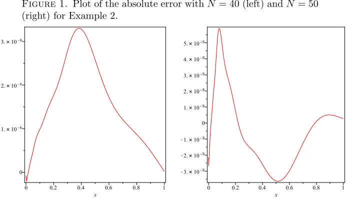
Example 2. Let us solve the following Bagley-Torvik equation [10]
y(2)+ 8 17y
(3/2)+13
51y=
x−1/2
89250√π
(
48p(x) + 7√πxq(x)), x∈[0,1],
where p(x) = 16000x4 −32480x3+ 21280x2−4746x+ 189 and q(x) = 3250x5− 9425x4+ 264880x3−448107x2+ 233262x−34578.Here, the boundary conditions are y(0) = 0 andy(1) = 0. It can be easily verified that the exact solution is
y(x) =x5−29 10x
4+76
25x
3−339
250x
2+ 27
125x.
The absolute errors are obtained in Table 1 for different values ofN using the pre-sented method. Also, Figure 1 shows the plot of absolute error withN= 40,50.
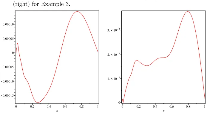
Example 3. In our third example, we consider the equation [6]
Figure 1. Plot of the absolute error withN= 40 (left) andN = 50 (right) for Example 2.
with the boundary conditions y(0) = 0 and y(1) = 1. The exact solution of this problem is given byy(x) =x2. Figure 2 shows the plot of absolute error withN = 32
andN = 64 using the presented method. Of course the accuracy of our method can be improved by increasingN.
Table 1. Absolute errors for different values ofN for Example 2.
x N = 8 N = 16 N = 32 N = 64 0.1 2.90×10⁻³ 2.96×10⁻⁴ 1.36×10⁻⁶ 3.92×10⁻⁹
0.2 9.92×10⁻⁴ 4.78×10⁻⁴ 4.17×10⁻⁶ 4.59×10⁻⁹
0.3 2.18×10⁻⁴ 6.26×10⁻⁴ 1.36×10⁻⁶ 4.16×10⁻⁹
0.4 3.83×10⁻⁴ 9.04×10⁻⁴ 5.30×10⁻⁶ 4.12×10⁻⁹
0.5 1.36×10⁻³ 1.13×10⁻³ 3.41×10⁻⁶ 3.87×10⁻⁹ 0.6 1.88×10⁻³ 1.18×10⁻³ 3.19×10⁻⁷ 3.82×10⁻⁹ 0.7 1.83×10⁻³ 1.03×10⁻³ 2.17×10⁻⁶ 4.54×10⁻⁹ 0.8 1.32×10⁻³ 7.44×10⁻⁴ 2.74×10⁻⁶ 4.78×10⁻⁹ 0.9 6.17×10⁻⁴ 3.79×10⁻⁴ 1.65×10⁻⁶ 3.16×10⁻⁹
5. Conclusion
Figure 2. Plot of the absolute error withN= 32 (left) andN = 64 (right) for Example 3.
Acknowledgment
The authors are very thankful to reviewers for carefully reading the paper and for their comments and suggestions.
References
[1] Y. Cenesiz, Y. Keskin, and A. Kurnaz,The solution of the Bagley-Torvik equation with the generalized Taylor collocation method, J. Franklin Inst.,347(2010), 452-466.
[2] S. Das,Functional Fractional Calculus for System Identification and Controls, Springer, New York, 2008.
[3] S. Esmaeili, M. Shamsi, and Y. Luchko,A pseudo-spectral scheme for the approximate solution of a family of fractional differential equations, Commun. Nonlinear Sci. Numer. Simulat., 16 (2011), 3646-3654.
[4] N. Hale and A. Townsend,Fast and accurate computation of Gauss-Legendre and Gauss-Jacobi quadrature nodes and weights, SIAM J. Sci. Comput.,35(2013), A652-A674.
[5] S. Irandoust-pakchin, H. Kheiri, and S. Abdi-mazraeh,Efficient computational algorithms for solving one class of fractional boundary value problems, Comput. Math. and Math. Phys.,53 (2013), 920-932.
[6] M. F. Karaaslan, F. Celiker, and M. Kurulay,Approximate solution of the Bagley-Torvik equa-tion by hybridizable discontinuous Galerkin methods, Appl. Math. Comput.,285(2016), 51-58. [7] A. A. Kilbas, H. M. Srivastava, and J. J. Trujillo,Theory and Applications of Fractional
Dif-ferential Equations, Elsevier, San Diego, 2006.
[8] M. Lakestani, M. Dehghan, and S. Irandoust-pakchin,The construction of operational matrix of fractional derivatives using B-spline functions, Commun. Nonlinear Sci. Numer. Simulat.,17 (2012), 1149-1162.
[10] S. Mashayekhi and M. Razzaghi,Numerical solution of the fractional Bagley-Torvik equation by using hybrid functions approximation, Math. Meth. Appl. Sci.,39(2016), 353-365.
[11] K. S. Miller and B. Ross,An Introduction to The Fractional Calculus and Fractional Differential Equations, Wiley, New York, 1993.
[12] A. Mohebbi, M. Abbaszadeh, and M. Dehghan, Compact finite difference scheme and RBF meshless approach for solving 2D Rayleigh-Stokes problem for a heated generalized second grade fluid with fractional derivatives, Comput. Methods Appl. Mech. Engrg.,264(2013), 163-177. [13] A. A. Neamaty, B. Agheli, and M. A. Firozja,Numerical solution for boundary value problem
of fractional order with approximate integral and derivative, Comput. Methods Differential Equations,2(2014), 195-204.
[14] K. B. Oldham and J. Spanier,The Fractional Calculus, Academic Press, New York, 1974. [15] K. Parand, M. Dehghan, and A. Pirkhedri,The Sinc-collocation method for solving the
Thomas-Fermi equation, J. Comput. Appl. Math.,237(2013), 244-252.
[16] I. Podlubny,Fractional Differential Equations, Academic Press, San Diego, 1999.
[17] S. S. Ray, On Haar wavelet operational matrix of general order and its application for the numerical solution of fractional Bagley-Torvik equation, Appl. Math. Comput., 218 (2012), 5239-5248.
[18] A. Saadatmandi, Bernstein operational matrix of fractional derivatives and its applications, Appl. Math. Modelling,38(2014), 1365-1372.
[19] A. Saadatmandi, A. Asadi, and A. Eftekhari,Collocation method using quintic B-spline and sinc functions for solving a model of squeezing flow between two infinite plates, Int. J. Comput. Math.,93(2016), 1921-1936.
[20] A. Saadatmandi and M. Dehghan,Numerical solution of a mathematical model for capillary formation in tumor angiogenesis via the tau method, Commun. Number. Math. Eng.,24(2008), 1467-1474.
[21] A. Saadatmandi and M. Dehghan,A new operational matrix for solving fractional-order differ-ential equations, Comput. Math. Appl.,59(2010), 1326-1336.
[22] A. Saadatmandi and M. Dehghan,A tau approach for solution of the space fractional diffusion equation, Comput. Math. Appl.,62(2011), 1135-1142.
[23] A. Saadatmandi, M. Dehghan, and M. R. Azizi,The Sinc-Legendre collocation method for a class of fractional convection-diffusion equations with variable coefficients, Commun. Nonlinear Sci. Numer. Simulat.,17(2012), 4125-4136.
[24] A. Saadatmandi and M. Razzaghi,The numerical solution of third-order boundary value prob-lems using Sinc-collocation method, Commun. Numer. Meth. Engng,23(2007), 681-689. [25] A. Saadatmandi, M. Razzaghi, and M. Dehghan,Sinc-collocation methods for the solution of
Hallen’s integral equation, J. of Electromagan. Waves and Appl.,19(2005), 245-256.
[26] F. Stenger,Numerical Methods Based on Sinc and Analytic Functions, Springer-Verlag, New York, 1993.
[27] S. Yeganeh, A. Saadatmandi, F. Soltanian, and M. Dehghan, The numerical solution of differential-algebraic equations by sinc-collocation method, Comput. Appl. Math., 32 (2013), 343-354.