Universitá degli Studi di Trento
Study of dynamic and
ground-state properties
of dipolar Fermi gases
using mean-eld and
quantum Monte Carlo methods
Ph.D. thesis by
Natalia Matveeva
Thesis advisor: Prof. Stefano Giorgini
Facoltá di Scienze Matematiche Fisiche e Naturali
Dipartimento di Fisica
Contents
1 Introduction 1
1.1 Ultracold dipolar gases . . . 3
2 Dipolar drag in bilayer harmonically trapped gases 9 2.1 Introduction . . . 9
2.2 Dipolar drag of the center-of-mass motion . . . 10
2.3 The model and the method . . . 11
2.4 The details of calculations . . . 13
2.5 Variational parameters . . . 14
2.5.1 Bosons . . . 14
2.5.2 Fermions . . . 16
2.6 Frequency shift: bosons versus fermions . . . 16
2.7 Comparison with a classical gas . . . 17
2.8 Conclusions . . . 18
3 Quantum Monte Carlo methods 21 3.1 Introduction . . . 21
3.2 Basic concepts . . . 24
3.3 Random walks and Metropolis sampling . . . 27
3.4 Variational Monte Carlo . . . 31
3.5 Diusion Monte Carlo . . . 34
3.6 Diusion Monte Carlo for fermions . . . 40
3.7 Trial wave functions . . . 41
3.8 Correlation functions . . . 42
4 Liquid and Crystal Phases of Dipolar Fermions in Two Di-mensions 49 4.1 Introduction . . . 49
4.2 Calculation of the potential energy . . . 51
4.3 Fermi liquid phase . . . 53
4.3.1 General physical properties of a Fermi liquid and the Slater-Jastrow wave function . . . 53
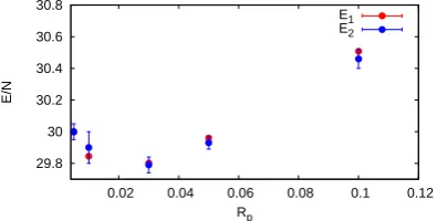
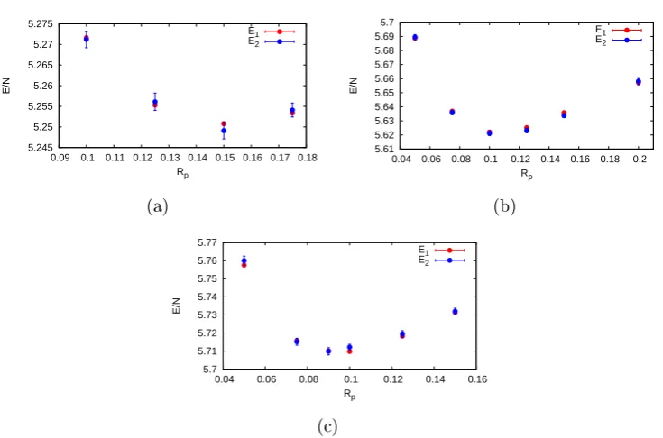
4.3.2 Optimization of the variational parameter Rp . . . 54
4.3.3 Optimization of DMC parameters: time step and num-ber of walkers . . . 55
4.3.5 Equation of state, eective mass and renormalization
factor . . . 58
4.3.6 Chemical potential and compressibility . . . 61
4.4 Crystal phase . . . 62
4.4.1 Wave function . . . 62
4.4.2 Optimization of the variational parameter α . . . 63
4.4.3 Finite size scaling . . . 63
4.5 Stripe phase . . . 64
4.5.1 The model . . . 64
4.5.2 VMC results . . . 66
4.5.3 Finite size scaling . . . 66
4.6 Quantum phase transition liquid-crystal . . . 67
4.7 Correlation functions . . . 69
5 The impurity problem 75 5.1 Introduction . . . 75
5.2 Two-body problem . . . 76
5.3 Perturbative calculation of the impurity chemical potential. . . 79
5.4 Trial wave function and its optimization . . . 81
5.5 Calculation of the potential energy . . . 82
5.6 Chemical potential of the impurity . . . 83
5.7 Eective mass of the impurity . . . 85
5.8 Conclusion . . . 85
Acknowledgements
I would like to express my deep gratitude to my supervisor Prof. Stefano Giorgini for his great scientic support, condence, kindness, patience and encouraging me. His willingness to give his time so generously has been very much appreciated. Also I am very grateful to Prof. Sandro Stringari and Alessio Recati with who I've been working during the rst year of the PhD study.
I would like to thank all members of INO-CNR BEC center with who I al-ways had very useful and interesting discussions, especially Gianluca Bertaina, Riccardo Rota, Marta Abad, Yun Li, Marco Larcher, Giovanni Martone, Luis Ardila, Yan-Hua Hou, Nicola Bartolo, Robin Scott, David Papoular, Tomoki Ozawa, Zou Peng, Gabriele Ferrari, Giacomo Lamporesi, Onur Umuncalilar, Phillipp Hyllis, Francesco Piazza, Michael Klawunn. It was a great opportu-nity to spend three years in such an inspiring place. I would also like to extend my thanks to the secretaries Beatrici Ricci, Michaela Paoli, Flavia Zanon and the technician Giuseppe Froner.
Also I am very grateful to the group of Prof. Jordi Boronat in UPC, Barcelona and especially to Gregory Asrtracharchik for the hospitality during my visit, for many valuable advices and useful critiques.
The discussions with Prof. Markus Holzmann, Sebastiano Pilati and Alex Pikovski are also greatly appreciated.
Chapter 1
Introduction
In this thesis we theoretically study the dynamic and ground state prop-erties of ultracold dipolar Fermi gases. Since 1995, when a Bose-Einstein condensate was experimentally created [1, 2], the eld of ultracold gases has been developing very rapidly. The rst degenerate Fermi gas has become experimentally available since 1999 [3] and during the last ten years a spec-tacular experimental progress has been achieved in the creation of Bose and Fermi gases with dipolar interactions (see Section 1.1). A lot of theoreti-cal studies devoted to ultracold gases with short- and long-range interactions were performed as well. Several reviews are available: Bose [4] and Fermi [5] gases with short-range interactions, Bose [6] and Fermi [7] gases with dipolar interactions.
The interest in ultracold atoms is based on the fact that they are highly controllable and clean systems and they can be used to verify with great pre-cision condensed-matter theoretical predictions. This task has already been largely accomplished in the case of the short-range interactions, but systems with dipolar interaction can give access to a wider range of physical phenom-ena. As an example, in the near future they can be used to simulate solid state systems with long-range interactions similar to Coulomb case. The new interesting features of the dipolar interaction is the possibility of controling its strength and the anisotropic character.
In the weakly interacting regime, the mean-eld approach and perturba-tion theory can be used to study the ground-state and dynamic properties of ultracold gases. These approaches, however, have the disadvantage that they become inaccurate with the increase of the interaction strength. Therefore, more precise numerical techniques, such as the Quantum Monte Carlo meth-ods (QMC), are better suited to investigate the strongly interacting regime. These methods allow one to nd the exact ground-state energy of a many-body Hamiltonian for bosonic systems and a very good upper bound of the ground-state energy for fermionic ones. The investigation of dynamic prop-erties using the QMC methods is computationally very demanding and the majority of the QMC studies are devoted to the ground-state properties.
method (FNDMC) is used instead to investigate the ground-state properties of two dimensional dipolar Fermi gases. This technique is also applied to the problem of one impurity in a bilayer conguration with dipolar fermions.
In the rst project a trapped bilayer conguration of a dipolar Fermi gas is studied (Chapter 2). Due to the long-range character of the dipolar interaction a frequency shift of the collective dipole mode is expected. This shift can open the possibility to experimentally measure the parameters of the dipolar potential. Our goal is to propose a scheme of a drag experiment (analogous to the famous Coulomb drag experiment), which can be realized using dipolar Fermi gases. We found that this eect is relatively large and can be detected in a sample of polar molecules.
Chapter 3 contains the detailed description of the QMC methods which we use, namely the Variational and the Diusion Monte Carlo techniques.
The second project, which is discussed in Chapter 4, is devoted to the study of the ground-state properties of a two dimensional dipolar Fermi gas at zero temperature by means of the FNDMC method. The dipoles are ori-ented by an external eld perpendicular to the plane of motion, resulting in a purely repulsive 1/r3 interaction. In the weakly interacting regime the ground
state of the system can be described in terms of the Fermi liquid theory. We calculated the ground-state energy, the eective mass of a quasiparticle and the renormalization factor of the momentum distribution. In the strongly interacting regime the system is expected to undergo the transition to a crys-talline phase. The point of this quantum phase transition was quantitatively established. Near the phase transition point we also searched for the existence of a stripe phase predicted by dierent mean-eld approaches. It was found that this phase is never energetically favorable. Also, important quantities related to the system, such as the pair-distribution function, the static struc-ture factor and the momentum distribution were obtained for a wide range of parameters.
In Chapter 5 we discuss 2D dipolar fermions in a bilayer conguration, where the dipole moments are polarized perpendicular to the planes. We con-sider the case of only one particle in the top layer and many particles in the bottom layer which are in the Fermi liquid phase. The intralayer interaction has a purely repulsive 1/r3 character, but the interlayer one has an
attrac-tive part. This system represents an interesting impurity problem with long-range anisotropic interactions. Using the FNDMC method we calculated the chemical potential of the impurity, its eective mass and the pair-correlation function between the impurity and the bottom layer particles.
1.1. Ultracold dipolar gases 3
the eld of ultracold dipolar gases and the new physical phenomena which appear due to the long-range character of the dipolar interaction.
1.1 Ultracold dipolar gases
As it follows from the basic principles of quantum mechanics, a particle can be described as a matter wave packet with the characteristic de Broglie wave lengthλT =
q
~
2πmkBT, whereT is the temperature, mis the atomic mass and
kBis Boltzmann's constant. At densityn '1012cm−3and at temperatureT ' 10−6K, the mean interparticle distancel = 1/n3 is comparable or less thanλ
T
meaning that the matter waves of the dierent particles overlap and quantum indistinguishability becomes important. If these conditions are satised, a gas is in the quantum degenerate regime. It means that the eects of quantum statistics play an important role. If the temperature of an atomic ensemble is less than a critical temperature a Bose gas forms a Bose-Einstein condensate, while a Fermi gas enters gradually the degenerate regime by reducing the temperature. For a detailed description of these states of matter see the reviews [4] and [5].
If the particles of an ultracold gas do not have a dipole moment, the s-wave scattering is the dominant process. Therefore, the real interatomic potential (typically the van der Waals interaction) can be eectively replaced by the contact interaction potential
Ucont(r) =
4π~2a
m δ(r) = gδ(r), (1.1)
where a is the s-wave scattering length. As one sees from Eq. (1.1), the
contact potential is isotropic, short-range and is characterized only by the value of the scattering lengtha. Notice that for a single-component Fermi gas
the potential (1.1) is absent and only p-wave interactions are allowed by the Pauli principle.
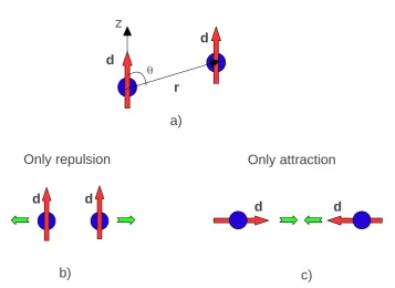
If the particles have a dipole moment their interaction include both the contact and the dipolar part. Assuming that the dipoles are polarized by an external eld (electric or magnetic) along the z-axis (see Fig. 1.1.a), the
dipolar interaction has the following form
Vdd(r) =
d2
r3(1−3 cos
2θ). (1.2)
Here d is the electric (magnetic) dipole moment, r is the vector connecting
two particles, and θ is the angle between r and the direction of d (z-axis).
Figure 1.1: Two aligned dipoles (a), "side-by-side" conguration, purely repul-sive interaction (b), "head-to-tail" conguration, purely attractive interaction (c).
with respect to r, the dipolar potential Vdd can be completely repulsive (Fig.
1.1.b), completely attractive (Fig. 1.1.c) or partially repulsive and partially attractive. The other important property of Vdd is its long-range character,
which appears because, from Eq. (1.2), it decays as 1
r3 at large distances. Such long-range behavior leads to scattering properties dierent from the contact interaction case. As it was found in Ref. [10], for the dipole-dipole interaction the phase shift δl in a scattering channel with angular momentum l behaves
as δl ∼k forl ≥0 and small k and therefore all partial waves must be taken
into account.
The other important characteristic of the dipolar potential is the existence of a contribution to the s-wave scattering channel. It appears because, due to the anisotropy of Vdd, the angular momentum is not conserved during the
1.1. Ultracold dipolar gases 5
s-wave contribution to the scattering amplitude is equal to zero due to the Pauli exclusion principle and the long-range dipolar part of the interaction alone denes the scattering properties.
In the weakly interacting regime the following pseudopotential was pro-posed in Ref. [11] to describe the properties of a polarized ultracold dipolar gas of bosons
Vpseud(r) =gδ(r) +
d2
r3(1−3 cos 2
θ), (1.3)
where
g = 4π~
2a
m . (1.4)
Hereais the s-wave scattering length. It is worth noticing here that the dipolar
potential (the second term in the right-hand side of Eq. (1.3) also contributes to the s-wave scattering and therefore modies the s-wave scattering lengtha.
For a one-component Fermi gas the pure dipolar potentailVdd is used instead
of Eq. (1.3).
The strength of the dipolar interaction can be characterized by the quan-tity
r0 =
md2
~2 . (1.5)
The scale ofr0 in Eq. (1.5) has the dimension of length and it can be
consid-ered as the characteristic length of the dipolar interaction.
The other important property of the dipolar interaction is its tunability. There are possibilities to tune the strength and the sign of the dipolar interac-tion [12] as well as its shape [13, 14] using a combinainterac-tion of external magnetic and electric elds.
Let us discuss now the experimental progress in the eld of ultracold dipo-lar gases. There are several possibilities to experimentally realize an ultracold gas with a dominant dipolar interaction. On one hand, one can work with atomic species having a large magnetic momentµ. At the present time several
of them are already available in the quantum degenerate regime. They are the following bosonic and fermionic atomic species: 52Cr [15] with µ = 6µ
B,
168Er [16] with µ= 7µ
B, 164Dy [17] and 161Dy withµ= 10µB [18] (where µB
is Bohr magneton). The magnetic interaction can be made stronger than the short-range one by tuning the eective scattering length close to zero using Feshbach resonances [19].
The second possibility to obtain a dipolar gas is the creation of heteronu-clear polar molecules. In their lowest rovibrational state such molecules can have an induced dipole moment along the internuclear axis as large as0.1−10 debye (D), where1D= 107.92µB. For comparison, the dipole moments
D, respectively. The most spectacular progress was obtained with 40K87Rb
fermionic molecules [20, 21, 22], which have a dipole momentd= 0.56D. The
experimental technique can be described as follows: potassium and rubid-ium atoms are brought to quantum degeneracy, then large and very weakly bound Feshbach molecules are created by tuning the interaction close to the resonance. These molecules, which have a very small dipole moment are trans-fered to the rovibrational ground state, where the dipole moment can reach its maximum value. The main problem with KRb molecules is the process of two-body losses which occur due to the possibility of the following isothermal chemical reaction
KRb+KRb→K2+Rb2. (1.6)
At present, a three-dimensional gas of KRbmolecules is available in the
quan-tum degenerate regime, but the molecules have a dipole moment d = 0.2D.
For larger values of d, a two-body losses increases exponentially due to the
chemical reaction (1.6). In a 2D geometry, the losses are greatly suppressed, but the gas is not yet available in the quantum degenerate regime (the lowest obtained temperature is T = 2.4TF). Other heteronuclear molecules can have
a dipole moment on the order of several debye. Currently, there are exper-imental attempts to create and bring to quantum degeneracy the following molecules: NaLi [23], NaK [24], LiCs [25] and RbCs [26].
Finally, let us mention a dipolar gas of Rydberg atoms [27, 28]. These atoms have a large dipole moment because they are in a highly exited elec-tronic state. The disadvantage of Rydberg atoms is a very short life-time compared to the case of magnetic atoms and dipolar molecules.
Such a spectacular experimental development goes alongside with the the-oretical progress. We briey discuss some of the thethe-oretical works, which are devoted to homogeneous and trapped systems, without considering lattice models (e. g. Bose-Hubbard model). For a general review see Ref. [7].
The ground-state properties of a spatially homogeneous and a trapped dipolar Bose gas were studied within the mean-eld approximation in Refs. [29, 30, 31, 32]. It was found that a bulk system with a dominant dipo-lar interaction is always unstable against collapse. However, a trapped Bose gas can be stabilized when the number of particles is smaller than a critical number. The analysis of the excitation spectrum of a trapped Bose gas was performed using the time-dependent Gross-Pitaevskii equation [29, 33, 34] and the Bogoliubov- de Gennes equations [32]. For a very anisotropic pan-cake trap, with the dipoles perpendicular to the trap plane, the excitation spectrum has a roton-maxon shape similar to that in superuid helium [35].
Dipolar weakly-interacting homogeneous Fermi gases with purely 1/r3
1.1. Ultracold dipolar gases 7
with modied Landau parameters. The anisotropy of the dipolar interac-tion leads to the anisotropy of the Fermi surface and, correspondingly, of the Fermi liquid parameters. This eect was investigated in Refs. [37, 38], using the Hartree-Fock approximation. It was also found that the anisotropy of the Fermi surface results in the appearance of a stripe phase [39, 40] characterized by stationary density modulations.
Chapter 2
Dipolar drag in bilayer
harmonically trapped gases
We consider two separated pancake-shaped trapped gases interacting with a dipolar (either magnetic or electric) force. We study how the center of mass motion propagates from one cloud to the other as a consequence of the long-range nature of the interaction. The corresponding dynamics is xed by the frequency dierence between the in-phase and the out-of-phase center of mass modes of the two clouds, whose dependence on the dipolar interaction strength and the cloud separation is explicitly investigated. We discuss Fermi gases in the degenerate as well as in the classical limit and comment on the case of Bose-Einstein condensed gases. This chapter shares the main results with Ref. [8].
2.1 Introduction
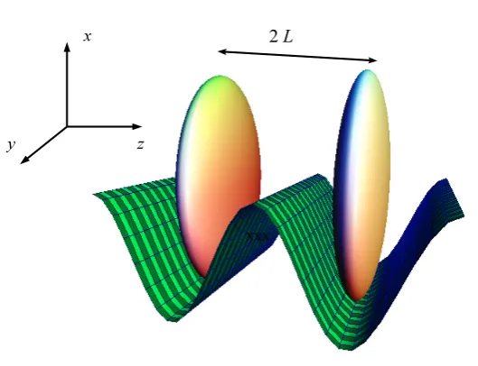
The aim of the present work is to propose a drag experiment induced by the long-range nature of the dipolar interaction. We consider an atomic or molecular gas harmonically trapped in a double well conguration such that the overlap between the two clouds and the corresponding tunneling eect can be neglected (see Fig. 2.1). The only force acting between the two gases is of long-range nature (here and in the following we assume that dipoles are oriented in the direction orthogonal to the discs, i.e along the z-th axis
Figure 2.1: Scheme of two not overlapping pancake shaped clouds of a dipolar gas. The distance between the centers of mass of the clouds is 2L. The clouds
are harmonically conned in the transverse directions x,y.
2.2 Dipolar drag of the center-of-mass motion
We consider a gas conned by a cylindrically harmonic potential:
Vtrap1,2(x, y, z) = 1
2mω
2
⊥[x2+y2+λ2(z±z0)2]. (2.1)
where 2z0 is the distance between the minima of the potential along z,
λ = ωz/ω⊥ is the ratio between the transverse and longitudinal trapping
frequencies and we consider pancake congurations, i.e., λ 1. Let xi being
the center of mass coordinate along x of the i-th cloud. The equations of
motion can be written as
d2x 1
dt2 =− ω 2
⊥x1−α(x1−x2), (2.2)
d2x 2
dt2 =− ω 2
⊥x2+α(x1−x2), (2.3)
where α is the coupling between the two bare center-of-mass modes. The
eigenfrequencies of the previous equations are simply ωin = ω⊥, for the
in-phase sloshing mode andωout =ω⊥
p
1 + 2α/ω2
⊥ for the out-of-phase sloshing mode. Thus in order to determine α we just need to determine the splitting ωout−ω⊥for the dipolar coupled system. Once the frequencyωout is known, we
2.3. The model and the method 11
0 0.02 0.04 0.06 0.08 0.1
t [s] -1
-0.5 0 0.5 1
x1 /x1
(t=0)
0 0.02 0.04 0.06 0.08 0.1
t [s] -1
-0.5 0 0.5 1
x2 /x2
(t=0)
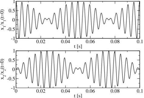
Figure 2.2: The motion of the center of mass of the two clouds for ωout = 1.1ω⊥, with ω⊥/2π = 200 Hz which corresponds to a beating time ¯t =
π/(ωout − ω⊥) = 0.025s. Initially, at t = 0, only the cloud 1 is displaced
from its central equilibrium position.
is shown. The beating of the motion is a direct measurement of the out-of-phase mode frequency, since the time at which the initially displaced cloud stops in the center is simply ¯t=π/(ωout−ω⊥).
In the following we calculate the frequencyωoutas a function of the dipolar
interaction strength and the distance between the two clouds. We will also discuss how the equation of state of the gas aects such a frequency. The frequencyωout was recently calculated by Huang and Wu [51] in the case of a
magnetic dipolar Bose gas, using a technique very similar to the one employed in the present work. For this reason we mainly focus on the case of a Fermi gas. Moreover the Fermi statistics allows for an easier realization of cold gases of hethero-nuclear molecules carrying an electric dipole moment (e.g., the recent experiment [22]) so that the strength of the dipolar force can be much larger.
2.3 The model and the method
We consider two clouds of dipolar ultracold gas (Fig. 2.1), each cloud is conned in the cylindrically harmonical potential (2.1).
The dipoles are oriented along the axis z by an additional external eld.
The interaction potential between two dipoles (d~1 =d~2 =d~) has the standard
form:
VD(r~1, ~r2, θ) =
d2(1−3 cos2θ)
|r~1 −r~2|3
, (2.4)
The energy functional for the system has the following general form:
E[na, nb] =E[na] +E[nb] +
Z
d~rad~rbVD(~ra−~rb)na(~ra)nb(~rb), (2.5)
where na and nb are the atomic densities for clouds a and b, ~ra and ~rb are
the coordinates relative to the two clouds, E[na] and E[nb] are the energy
functionals of each cloud separately.
Let us consider the small density shifts along the x axis of cloud a and
cloud b:
na,b(x, y, z)→na,b(x−εa,b, y, z). (2.6)
We can write the variation of the energy (2.5) as a dierence between the energy of shifted and nonshifted position:
δE =E[na(x−εa, y, z), nb(x−εb, y, z)]−E[na(x, y, z), nb(x, y, z)]. (2.7)
From the other hand for small oscillations the expression (2.7) is equal to the potential energy:
δE =mω2DN(ε2a+ε2b), (2.8)
where ωD is the frequency of the dipole mode andN is the number of atoms
in each cloud. Provided that the frequency shifts εa and εb are small the
expansion of expression (2.7) up to second order can be performed giving the result
na,b(x−εa,b)≈na,b−εa,b
∂na,b ∂x + 1 2ε 2 a,b
∂2n
a,b
∂x2 +.... (2.9)
After substitution Eq. (2.9) into Eq. (2.7) we obtain the following expression for δE:
δE = 1
2mω
2
pN(ε
2
a+ε
2
b)−
1
2(εa−εb)
2
Z
d~rad~rbVD(~ra−~rb)
∂na(~ra)
∂xa
∂nb(~rb)
∂xb
.
(2.10) It can be seen from Eq. (2.10) and Eq. (2.8) that for the in-phase mode (εa = εb) the frequency of the collective oscillation ωD equals the trap
fre-quency ωp. But, for the out-of-phase mode (εa = −εb) the frequency of the
dipole mode is dierent from the trap frequency:
ωD =ωp
1− 2
mω2
pN
Z
d~rad~rbVD(~ra−~rb)
∂na(~ra)
∂xa
∂nb(~rb)
∂xb
1/2
. (2.11)
2.4. The details of calculations 13
2.4 The details of calculations
Let us denote by I the integral in Eq. (2.11)
I = Z
d~rad~rbVD(~ra−~rb)
∂na(~ra)
∂xa
∂nb(~rb)
∂xb
. (2.12)
It can be rewritten in the following way using the properties of the Fourier transformation and of the convolution:
I =
Z
d~ra
VD ∗
∂nb(~rb)
∂xb
(~ra)
∂na(~ra)
∂xa =
= Z
d~kF[VD∗
∂nb(~rb)
∂xb
](~k)F[
∂na(~ra)
∂xa
](~k) =
= Z
d~kF[VD](~k)F[
∂na(~ra)
∂x ](~k)F[
∂nb(~rb)
∂x ](~k), (2.13)
where the symbol ∗ denotes the convolution and F[. . .] is the Fourier trans-formation. The Fourier transformation of dipole potential [33] can be approx-imated as
F[VD](~k) = 4πd2(1−3 cos2α)
cos(bk) (bk)2 −
sin(bk) (bk)3
, (2.14)
where α is the angle between ~k and the dipole direction, and b is a cuto
distance corresponding to the atomic radius. Since b is much smaller than
any signicant length scale of the system, it is possible to perform the limit
lim
b→0F[VD(~r)] =
4π
3 d
2(3 cos2α−1). (2.15)
In the following we will always use Eq. (2.15).
To obtain the density distributions na(r~a) and nb(r~b) one needs to solve
the stationary non-local Gross-Pitaevskii equation with long-range dipolar interactions. In the present work we use the following Gaussian anzatz for the density:
na,b(x, y, z) =
N
W2
pWzπ
3 2
e−
(x2+y2) Wp2 −
(z2∓2zL+L2)
Wz2 , (2.16)
where 2L is the distance between layers a and b, while Wp and Wz are the
variational parameters that dene the size of the cloud. Using spherical coordinates I can be written as:
I = N
2d2
6π2
Z ∞
0
Z π
0
Z 2π
0
k4(3 cos2α−1) sin3αcos2φ×
×exp
−k2
2 sin
2
αWp2− W
2
zk2cos2α
2 + 2ıLkcosα
After the substitution cosα = y and the integration over φ Eq. (2.17)
becomes
I = N
2d2
6π2 I,˜
where ˜ I = Z ∞ 0 Z 1 −1
k4(1−y2)(3y2−1)×
×exp
−y2k2
2 (W
2
z −W
2
p)−
k2Wp2
2 + 2ıLky
dkdy.
Finally, the expression for ωD can be written as
ωd=ωp(1−
N d2
3πmω2
p ˜
I)1/2. (2.18)
2.5 Variational parameters
In this section we discuss the variational parameters of the Gaussian anzatz (2.16) which minimize the energy of a single cloud. The results of a Bose gas are also considered and compared to the ones of a Fermi gas.
2.5.1 Bosons
In the case of bosons the total energy for a single cloud has the following form [52]
Ebos =Etrap+Ekin+Econt+Edd, (2.19)
where Etrap =
R
nVtrapd~r is the potential energy due to the trap, Ekin =
~2
2m
R
∇n2d~r is the kinetic energy, E
cont = g2
R
n2d~r is the contact interaction
energy and
Edd = 1 2
Z
n(~r)n(~r0)Udd(~r−~r0)d~rd~r0
is the energy of dipolar interactions. By using the Gaussian anzatz (2.16) Eq. (2.19) becomes
Ebos =
mN ωp2
2 (W
2
p +
ω2
z 2ω2
p
Wz2) + N 4m(
2 W2 p + 1 W2 z ) + + N 2a √
2πmW2
pWz
− d2N2
3√2πW2
pWz
2.5. Variational parameters 15
where κ= Wp
Wz is the cloud aspect ratio, and
f(κ) = 1 + 2κ
2
1−2κ2 −
3κ2arctan√1−κ2
(1−κ2)3/2 .
As an example of a bosonic dipolar gas we consider 52Cr atoms (that
have relatively large magnetic dipole moment dCr = 6µB) and 41K87Rb polar
molecules. The rst case is important because BEC of 52Cr atoms has been
already created experimentally [15]. The second case is also very interesting because41K87Rb molecules have a large electric dipole moment (d
KRB = 0.6D)
in the rovibrational ground state and their fermionic counterpart (40K87Rb)
is already available experimentally in the degenerate regime [22].
In Table 2.1 the values ofWp,Wz are shown for dierent trap aspect ratios
(λ= ωz
ωp) in the case of
52Cr (forλ = 1.6 notice that the cloud is predicted to
be spherical). The other parameters are as follows: number of atoms 30000 and ω = 2π·800 Hz, where ω= (ω2
pωz)1/3 is the average trap frequency. The
scattering length is taken to be equal to 18a0, where a0 is the Borh radius,
ap =
p
~/mωp and az =
p
~/mωz are the oscillator lengths in the radial and
axial direction.
Table 2.1: Bosons. The size of cloud for 52Cr.
λ ωp
2π, Hz ωz
2π, Hz Wp,10−
4cm W
z, 10−5cm Wp
ap
Wz
az
1.6 684 1094 1.05 10 1.88 2.5
10 372 3720 2.5 3.2 2.8 1.4
20 295 5894 3.2 2.3 3.94 1.3
40 234 9356 3.9 1.6 4.28 1.1
The cloud size for the bosonic polar molecule 41K87Rb is shown in the
Table 2.2 at the same number of atoms and trap parameters (the caseλ= 1.6 absence because cloud is unstable for such parameters). The scattering length here is equal to100a0.
Table 2.2: Bosons. The size of cloud for 41K87Rb.
λ ωp
2π, Hz ωz
2π, Hz Rp, 10−
4cm R
z, 10−5cm Rapp Razz
10 372 3720 4.14 5 9 3.4
20 295 5894 5.6 2.8 10.8 2.4
2.5.2 Fermions
The total energy of a single cloud of dipolar fermions can be expressed in terms of the Thomas-Fermi energy functional [53]
Ef erm=
3 5
~2
2m(6π
2)2/3
Z
n5/3d3x+Edd+Epot, (2.21)
where Edd and Epot are the same as in the bosonic case. In the energy
func-tional (2.21) we have not included the intra-cloud exchange energy. We safely neglect it, because for the pancake-like congurations, which are our main interest, the direct term is the dominant eect (see, e.g., [37]).
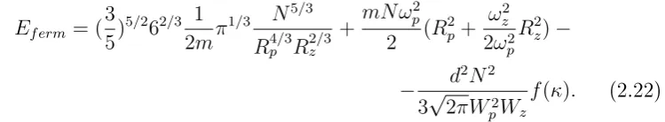
For the Gaussian anzatz (2.16)Ef erm becomes
Ef erm= (
3 5)
5/262/3 1
2mπ
1/3 N 5/3
R4p/3R2z/3
+mN ω
2
p
2 (R
2
p+
ωz2
2ω2
p
Rz2)−
− d2N2
3√2πW2
pWz
f(κ). (2.22)
In Table 2.3 the size of the cloud is shown for the fermionic polar molecules
40K87Rb. The trap parameters, the number of atoms and the scattering length
are taken to be the same as for the bosonic polar molecule 41K87Rb.
Table 2.3: Fermions. The size of cloud for 40K87Rb.
λ ωp
2π, Hz ωz
2π, Hz Rp, 10−
4cm R
z, 10−5cm Rp
ap
Rz
az
10 372 3720 4.64 5.28 10 3.6
20 295 5894 6.1 3.25 11.7 2.8
40 234 9356 7.84 2.02 13.4 2.18
From the comparison of Table 2.2 and Table 2.3 one sees that for the same trap parameters and value of the dipolar moment the fermionic cloud has a larger size compared to the bosonic one. This eect is a direct consequence of the Pauli exclusion principle.
2.6 Frequency shift: bosons versus fermions
In this section we study the frequency of the dipole mode (2.18) for bosonic (52Cr and 41K87Rb) and fermionic (40K87Rb) dipolar gases. We use the
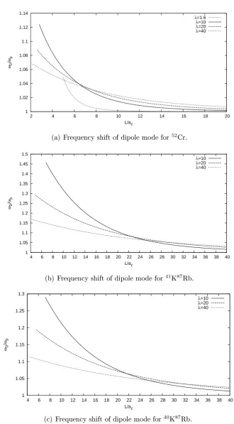
vari-ational parameters which were presented in the previous section. Fig. 2.3 shows the dependence ofωD on the distanceLbetween the clouds at dierent
2.7. Comparison with a classical gas 17
can see that the eect of the frequency shift is not too small (around several percents) and, in principle, can be experimentally detected. The middle and bottom gures depict the ωD for 41K87Rb and 40K87Rb polar molecules. The
eect is slightly larger for bosons than for fermions. This fact can be under-stood in the following way: as emerges from Eq. (2.11) the eect is amplied for smaller radial sizes where the gradient of the density is larger, and, as it was discussed above, the sizes Wp and Wz are smaller for a bosonic cloud.
Moreover, we see that for small enough distances the larger the cloud (largerλ for xedN) the smaller the eect. This can be easily understood in
terms of the potential of a single disk of radiusW⊥ on a probe dipole. Indeed
at a distance z W⊥ the potential decays with W⊥, which is a general result
independent of statistics. On the other hand we have that the asymptotic behavior of the frequency shift at large distance is ∝ p1 +C/L5 with C a
constant, which is the result one immediately obtains by considering just two trapped dipoles. It can also be easily shown that for spherical clouds with
W⊥ =Wz =W in Eq. (2.11) the frequency of the out-of-phase dipole mode
reads
ωout =ω⊥ 1−
√
2N d2h(L/W)
3√πmω2
⊥L5 !1/2
, (2.23)
whereh(y) = e−2y2(4y5+ 6y3+ 9/2y)−9/2pπ2Erf(√2y), which approaches a constant for large values of y.
2.7 Comparison with a classical gas
An important question arises: is it possible to detect the frequency shift of dipolar mode for a classical gas? This section is devoted to the comparison of ωD for a degenerate Fermi gas of 40K87Rb molecules with a classical gas
composed of the same molecules. Here we chose other parameters for the trap and number of particles, which should be closer to the parameters of the 41K87Rb experiment [22]. The Tables 2.4 and 2.5 show the variational
parameters for degenerate and classical gases, correspondingly. There TF ≡ ~ω⊥(6N λ)1/3/k
B is the Fermi temperature and kB is Boltzmann's constant.
For a classical gas we use simply the Gaussian density proles of Eq. (2.16) where the radii are given by the Boltzmann expression W2
⊥ = 2kBT /(mω⊥2)
and κ=λ.
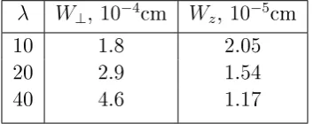
In Fig. 2.4 and Fig. 2.5 we report the predictions for the frequency shifts exhibited by the degenerate gas and the thermal conguration calculated at the temperature T = TF. The variational parameters are taken from Tables
Table 2.4: The cloud size for N = 2200 40K87Rb molecules with ωz/2π = 10
kHz (corresponding to az = 8.89×10⁻⁶cm) and dipole momentum d = 0.56
D.
λ W⊥,10−4cm W
z,10−5cm
10 1.8 2.05
20 2.9 1.54
40 4.6 1.17
Table 2.5: The size of cloud for classical gas of 40K87Rb at T = T
F with
dipole momentum d = 0.56D and trapping frequency ωz = 10 kHz (az = 8.89×10⁻⁶cm).
λ W⊥,10−4cm Wz,10−5cm
10 2.8 2.8
20 4.5 2.25
40 7.15 1.79
number of particles, is smaller for a classical gas than for a degenerate Fermi gas, since the thermal radii are larger and the densities smaller than the ones of the degenerate conguration.
2.8 Conclusions
2.8. Conclusions 19
1 1.02 1.04 1.06 1.08 1.1 1.12 1.14
2 4 6 8 10 12 14 16 18 20
ωD
/
ωp
L/az
λ=1.6
λ=10
λ=20
λ=40
(a) Frequency shift of dipole mode for52Cr.
1 1.05 1.1 1.15 1.2 1.25 1.3 1.35 1.4 1.45 1.5
4 6 8 10 12 14 16 18 20 22 24 26 28 30 32 34 36 38 40 ωD
/
ωp
L/az
λ=10
λ=20
λ=40
(b) Frequency shift of dipole mode for41K87Rb.
1 1.05 1.1 1.15 1.2 1.25 1.3
4 6 8 10 12 14 16 18 20 22 24 26 28 30 32 34 36 38 40 ωD
/
ωp
L/az
λ=10
λ=20
λ=40
(c) Frequency shift of dipole mode for40K87Rb.
Figure 2.3: Frequency shift of dipole mode for bosons: 52Cr (a),41K87Rb (b);
5 10 15 20 25 30 35 L/az
1 1.05 1.1 1.15 1.2 1.25 1.3
ωout
/
ω⊥
λ = 10 λ = 20 λ = 40
Figure 2.4: Frequency shift of ωout/ω⊥ for the out-of-phase mode for a
degen-erate gas of 40K87Rb, with parameters as given in Table 2.4.
5 10 15 20 25 30 35
L/az 1
1.01 1.02 1.03 1.04
ωout
/
ω⊥
λ = 10 λ = 20 λ = 40
Figure 2.5: Frequency shift ofωout/ω⊥for the out-of-phase mode for a classical
gas of 40K87Rb at temperature T = T
F, where TF is the Fermi temperature
Chapter 3
Quantum Monte Carlo methods
In this chapter we describe Quantum Monte Carlo methods and the under-lying concepts, such as Markov chains and Metropolis algorithm. We discuss Variational and Diusion Monte Carlo techniques, as well as trial wave func-tions used for bosonic and fermionic systems.
3.1 Introduction
The behavior of a nonrelativistic quantum system can be described by the many-body Schroedinger equation. The ground state expectation value of an operator can be found as a quantum-mechanical average on the many-body wave function that leads to the calculation of multidimensional integrals. Usually we are interested in the physical properties of a system which contains a large number of particles, so the problem of solving Schroedinger's equation as well as calculation of the observables becomes very dicult. If the degrees of freedom are strongly coupled, perturbation theories are not reliable and the use of dierent numerical techniques becomes necessary.
Monte Carlo (MC) methods are a class of techniques that are used to solve multidimensional integrals, where grid methods becomes ineective because the number of grid points rapidly increase with dimensionality. The essential property of MC methods is the stochastic nature, which arises from the use of random number sequences. More exactly, to compute the results, Monte Carlo methods rely on repeated random sampling which is governed by a probabil-ity distribution function. The term "quantum Monte Carlo" (QMC) covers several related stochastic methods that are used to investigate the properties of a variety of quantum systems. The word "quantum" is important since QMC approaches dier signicantly from Monte Carlo methods for classical systems.
Originally MC methods were developed mainly to study the properties of condensed matter systems. Historically the rst method was Variational Monte Carlo (VMC), which was used to study the ground-state properties of a bosonic isotope of helium, namely He4 [54]. In that method the modulus
upper bound of the ground-state energy (both for bosons and fermions) which crucially depends on the quality of the trial wave function used. The ground-state energy of liquid He4 was found to be in agreement with the experimental
value using more sophisticated wave functions [55]. VMC was also used to study the fermionic isotope3He ([55], [56]) and later to investigate the
ground-state properties of the electron gas. Later the Green's Function Monte Carlo (GFMC) method was developed and used for 4He [57] . For bosons GFMC
method samples a probability distribution proportional to the exact ground-state wave function, and it gives an exact ground-ground-state energy biased only by a statistical error, which can be decreased at the cost of simulation time. For fermions GFMC was rst used in [58]. Another method called Diusion Monte Carlo (DMC) was introduced in [59]. DMC solves the Schroedinger equation in imaginary time based on the short-time approximation of the Green function. It had allowed to signicantly improve the VMC results for the electron gas [61]. DMC is similar to GFMC but simpler in implementation which makes DMC a very popular method up to the present time (for review see [62]).
All techniques mentioned before are valid only at zero temperature. But there is the possibility to study nite temperature properties of quantum systems using Path Integral Monte Carlo methods (PIMC). They are based on the isomorphism between the partition function of quantum particles in the canonical ensemble representation and classical polymers. This partition function can be simulated using Monte Carlo algorithms. Firstly PIMC was used to study low-temperature properties of liquid 4He [63] and then became
a standard technique to study quantum liquids. Recently more sophisticated variants of PIMC were developed such as the Worm algorithm [64], which allows one to consider very large systems (up to several hundred thousands of bosons).
3.1. Introduction 23
Path-Integral technique discussed in [65], [66], deals with the sign problem at nite temperature.
During the last twenty years these methods were employed to study ultra-cold atomic systems. In the following we describe some of the most important QMC results. Initially, only systems with short-range contact interaction were studied.
We rst consider continuum systems. In Bose gases, beyond mean-eld corrections to the equation of state at zero temperature were calculated in three dimensions [67], two dimensions [68] and one dimension [69]. In fermionic systems, QMC approaches were used to give quantitative informa-tion about the BEC-BCS crossover [70], and especially the unitarity regime where there is no small parameter for perturbation theory. For example, the equation of state at zero temperature was calculated in [71] and in [72]. An-other interesting phenomena such as itinerant ferromagnetism was studied by means of the FNDMC method for a three dimensional repulsive Fermi gas [73], where evidence for a ferromagnetic phase was found.
Lattice models which are described by dierent variants of the Hubbard model also attracted a lot of attention. The Bose-Hubbard model [74], which is the simplest model that describes a conductor-insulator transition for bosons was the object of many studies. Such interest is based on the hope that bosons in optical lattices can play the role of quantum simulators for solid state systems (see Introduction). In [75] the superuid to normal liquid transition of the Bose - Hubbard model was experimentally investigated and benchmarked against the theoretical calculations. The integrated column densities from time-of-ight images showed excellent agreement with the results of the worm algorithm PIMC method over the whole temperature range. Remarkably, the QMC simulations were performed for 3∗ 105 bosons, the same number of
particles presenting in the experiment. Disordered Bose-Hubbard model for 3D bosons was studied by QMC methods in [76], [77]. The authors found that the Bose glass phase is an intermediate phase between the superuid and Mott insulator phases of the Bose-Hubbard model.
In the case of fermions the attractive Hubbard model was studied at uni-tarity in [78], [79], and the superuid transition temperature as well as the thermodynamic properties for unpolarized gases have been calculated.
in [45], [46]. It was found that at small densities the ground state of the system a liquid and at large densities a triangular crystal is formed. For 1/r3
interaction with a cut-o at small distances, the supersolid phase was instead predicted to appear at least in two dimensions [48]. This phase is formed through the formation of superuid droplets that become coherent as one lowers the temperature.
Finally, let us mention the Diagrammatic Monte Carlo method, which was developed to investigate the properties of fermionic systems at nite temper-ature. This method is based on a direct sampling of Fermi diagrams that contribute to physical properties. Recently, in [83] the equation of state of a balanced Fermi gas at unitarity was determined using this method.
3.2 Basic concepts
As it was already mentioned the most important use of Monte Carlo meth-ods is the calculation of multidimensional integrals. Non-stochastic methmeth-ods, such as grid methods are highly eective for low dimensional integrals or in case where the integrand can be approximately separated into low dimensional parts. But when the dimensionality d of the space increases the number of
grid points increases as Nd. For the cased≤5 some more sophisticated grid techniques can still be eective. But for higher dimensions the computational eorts increases so rapidly, that other possibilities such as Monte Carlo sam-pling become more favorable. Monte Carlo integration is based on samsam-pling points from an appropriate probability distribution function instead of using a grid.
Let us explain the idea of Monte Carlo evaluation of denite integrals. Only the one dimensional case is considered below, but the results can be easily generalized to the multidimensional case.
At the beginning, let us dene what is a random variable. Let us consider for example such process as throwing a dice. At each trial the result of this action can be expressed in term of a numerical value x which is called a
random variable. It can be discrete or take values in the continuum. The random variable is characterized by its domain and its probability distribution function (pdf), which also can be discrete or continuous. As an example, two common pdf's are written below. The rst one is the uniform distribution, dened in [a, b] as
f(x) = 1
(b−a)θ(x−a)θ(b−x), (3.1)
distri-3.2. Basic concepts 25
bution dened in (−∞,+∞)as
f(x) = √1
2πσexp
−(x−x¯)2
2σ2 . (3.2)
Usually we are not directly interested in the value of the variable xbut in
some function g(x). In this case the expectation value of g can be found as
< g >= Z b
a
g(x)f(x)dx, (3.3)
here it is assumed that x is dened in the interval (a, b). The important characteristics of a distribution are its mean valueµand central momentsµn.
Mean value is dened for g(x) = x as
< x >=µ= Z b
a
xf(x)dx (3.4)
and another choice of g(x) such as g(x) = (x−µ)n determines the central moments as
µn =
Z b
a
(x−µ)nf(x)dx. (3.5)
The second central momentµ2 is called the variance of the probability
distri-bution, usually its square root σ is used which corresponds to the standard
deviation.
Now we are ready to discuss the central limit theorem (CLT). Let us consider a random variable x with probability distribution f(x) which has mean value µand varianceσ. Also let us dene the random variablez as the
average overn random realizations of x:
z = x1+x2+...+xn
n . (3.6)
The CLT tells us that forn large enough the random variablez is distributed
according to the Gaussian distribution (3.2) independently of the form off(x). More exactly, the pdf p(z) of the random variablez is
p(z) = √1 2π
1
(σ/√n)exp(−
(z−µ)2
2(σ/√n)2). (3.7)
The mean of p(z) equals the mean of the original distribution f(x) and its variance is equal to the variance of f(x)divided by n.
So, the CLT proves that the mean of the probability distribution f(x) can be found as the average over n realizations of x. And the error in its
The importance of CLT is that it can be used not only for the calculation of the mean value of a probability distribution but can be easily generalized to other types of expectation values such as
mh =
Z b
a
h(x)f(x)dx, (3.8)
which has the variance
s2 = Z
f(x)(h(x)−µh)2dx. (3.9)
The generalized version of CLT tells us thatmh can be estimated as the mean
value of a new random variable
zh =
h(x1) +h(x2) +...+h(xn)
n . (3.10)
The variance of this estimate of mh is equal to the s2/n.
The most important use of CLT is the possibility to calculate dened integrals stochastically. Suppose we are interested in the calculation of the integral
I = Z b
a
h(x)dx, (3.11)
where h(x) is an arbitrary function (no necessarily positively dened). One can rewrite the integral I as
I = (b−a) Z b
a
h(x)f(x)dx, (3.12)
where f(x) is the uniform distribution (3.1). Now the integral I can be
con-sidered as the expectation value mh of h(x) on the distribution f(x)
I = (b−a)< h >u . (3.13)
According to CLT the expectation value < h >u can be estimated as the
average over a large numberN ofh(xi), wherexiare sampled from the uniform
distribution
< h >u≈¯h= 1
N
N
X
i=1
h(xi). (3.14)
The variance of this estimate of I is equal to
3.3. Random walks and Metropolis sampling 27
where for a nite number of samples
σ2h ≈ 1 N
N
X
i=1
(h(xi)−¯h)2. (3.16)
Therefore the variance in the estimate of the integral I equals
σI2 ≈ 1 N2
N
X
i=1
(h(xi)−¯h)2. (3.17)
One can see that the variance σ2
I depends on the variance of the function
h(x) and on the number N of samples. But the variance σ2
h depends only
on the shape of the function h(x). Therefore, the only way to reduce σI
is to increase N. This limitation can be overcome by using the importance
sampling technique, which allow one to signicantly reduce the variance of the integrand function.
In order to do this we should rewrite the integral (3.12) as
I = Z b
a
h(x)
q(x)q(x)dx=<
h(x)
q(x) >q, (3.18)
where h(x)
q(x) is the new integrand function and q(x) is the new (not uniform!)
distribution function such that q(x) is close to h(x). So, the integral can be estimated as
I ≈ h(x) q(x) =
1
N
N
X
i=1
h(xi)
q(xi)
, (3.19)
where the points {xi} are sampled from q(x). The probability to sample a
given point xi is larger where h(x) is large and smaller where h(x) is small,
which leads to smaller uctuations of h(xi)
q(xi) and, nally, to a decrease of the
variance with respect to the case of the uniform distribution.
3.3 Random walks and Metropolis sampling
In this section we discuss sampling from an arbitrary distribution function. In some cases the sampling can be done relatively easily, as, for example, for the Gaussian probability distribution (3.2), where the Box-Muller algorithm was developed [85]. Suppose we want to sample from a Gaussian distribution (3.2) withσ = 1andµ= 0. Firstly, one needs to sample two random variables
u1 andu2 from the uniform distribution (3.1) with a= 0 and b= 1 using, for
example, the standard algorithms ran2 or ran3 from [86]. Then, two variables
x1 and x2 should be calculated as
x1 =
p
−2 logu1cos(2πu2), x2 =
p
These variables x1 and x2 are independent random variables distributed
ac-cording to a Gaussian pdf. In case of arbitrary σand µ, the random variables x1,2 should be rescaled as x1,2 →σx1,2+µ.
In case of more sophisticated pdf's, usually there is no easy way to sample points from them. Metropolis and coworkers [87] developed a stochastic algo-rithm which generate asymptotically the given set of random numbers. This algorithm is based on a random walk in multidimensional space. Before going to the details of this algorithm we explain the underlying concept of Markov chain [84].
Firstly, let us dene a "walker" as a mathematical quantity which com-pletely describes the state of the system. The walker moves in congurational space by combination of deterministic and random displacements. Suppose the system has N statesS1, ..., SN such that the probability for the system to
occupy each of the states at a given time i ispi
1, ..., piN. All this probabilities
form the probability-space density, which can be represented as the vector
pi = [pi1...piN]T. (3.21)
If the system starts its evolution from the state Si, then after some time
it ends at Sf after a sequence of jumps between intermediate states. If at
every time the current state depends only on the previous one, then such a sequence of events is called a "Markov chain". The probability of the system to jump from state Sj toSk in one time step is dened as Pkj. The whole set
of probabilities {Pkj} forms so called transition probability matrix Pˆ. It is
obvious that its elements must satisfy the following conditions: 0 ≤ Pkj ≤ 1
and PjPkj = 1.
What happens to a system after a large number of jumps? Suppose that at time i the system is in the state Sj and then at the next time step i+ 1 it moves to Sk with probability Pkj. During this jump the probability
distribution changes aspik+1 =PjPkjpij, which can be written in a matrix form
aspi+1 = ˆPpi. Using this notation the evolution of the system from the initial
distribution can be written as follows: p1 = ˆPp0, then p2 = ˆPp1 = ˆPPˆp0
and so on. After m steps the probability-space density becomes pm = ˆPmp0.
If time m is suciently long|pm+1−pm| →0, which means that the system
has reached the equilibrium probability distribution p∗, dened as
p∗ = ˆPp∗. (3.22)
The probabilities p∗ can be found as the solution of the set of linear
3.3. Random walks and Metropolis sampling 29
The generalization of the discussed concept to the case of continuum space is called a Markov process. In this case the states can be labeled by the con-tinuous variable x0 and the transition probability can be dened as a function p(x, x0)with the properties p(x, x0)>0 and R p(x, x0)dx0 = 1.
Above we have considered a direct problem: how to get the stationary probability distribution which corresponds to a given transition probability matrix. But our sampling task requires the solution of the inverse problem: we should be able to nd an appropriate Pˆ for the desired p∗. This issue is addressed by the Metropolis algorithm [87, 88].
Assume the system is in state Si which has the equilibrium probability
p∗i. Then let us choose a trial state Sj which has the equilibrium probability
p∗j. The probability of transition between these two states is denoted as Qij,
where Qˆ could be an arbitrary matrix. If p∗
j > p∗i then the move is accepted
and the matrix element of the matrixPˆ isPij =Qij. Ifp∗
j ≤p∗i the trial state
is accepted with the probabilityp∗j/p∗i. In case the stateSj is not accepted the
new state is the old one. More precisely the above statements can be written as follows:
Pij = Qij, (p∗j > p∗i) (3.23)
Pij = Qijp∗j/p∗i, (p∗j ≤p∗i) (3.24)
Pii = Qii+
X
k,p∗k<p∗i
Qik(1−p∗k/p∗i) (3.25)
The last equation (3.25) is chosen in such a form to fulll the condition P
jPkj = 1.
It is worth to mention here that the matrix Pˆ constructed according to Eqs. 3.23, 3.24, 3.25 satises the detailed balance condition: Pkjp∗k = Pjkp∗j.
The transition probability matrix should satisfy this condition in order to produce a stationary probability distribution. So, the repeated actions of the matrix Pˆ drives the probability distribution to the equilibrium.
The Metropolis algorithm can be generalized to the case of continuous variables, which means that instead of the vectorp∗ we use now the function
p∗(x). In this case, to generate a random move one can use the continuous transition matrix W(xf in, xin)where xf in is given by
xf in =xin+D(2z−1), (3.26)
whereDis an arbitrary constant and z is a random variable sampled from an
uniform probability distribution. Suppose that at the initial time the system can be characterized by a vector xin, which contains the coordinates of all
easiest version of the Metropolis algorithm for continuous variables can be written as follows:
1. generate a random vector z from an uniform distribution
2. make an attempt move xin →xf in
3. ifp∗(xf in)≥p∗(xin)then go to step 5
4. if p∗(xf in) < p∗(xin) the new position xf in can be accepted with the
probability p(xf in)/p(xin) meaning that one needs to do the following
test:
i) generate a new random number z0 from an uniform distribution
ii) if p(xf in)/p(xin)> z0 then go to step 5
iii) if p(xf in)/p(xin)≤z0 the proposed positionxfin is not accepted and
we need to put xf in =xin
5. the new state isxf in
After many repetitions, we get a random number (vector) xfin sampled from
the desired probability distribution p∗(x).
It is important to mention the following. In the above algorithm the sta-tionary probability distribution is considered. But in practice the Metropolis algorithm gives the stationary distribution only after some equilibration time, so in order to use the points sampled fromp∗(x)one should wait an appropri-ate number of iterations. The parameter D inuences the acceptance rate A
of the random moves, which is dened as A= Nac
Ntot, whereNac is the number
of accepted moves and Ntot is the total number of attempts. In principle D
can be arbitrary, but if it is too small A is large, and many moves are needed
to cover the whole space; on the contrary if Dis too large A is small and the
system is stuck in each position for a large number of iterations. In both cases the equilibration time becomes too long. Therefore, the appropriate value of
D should be chosen empirically such that A= 0.5−0.7.
Another issue to address here is the number of walkers which is used in real simulations. As it was already mentioned the equilibrium random walk is an ergodic process, which, by denition, means that the temporal average can be replaced by the average on an ensemble. Therefore, we can use instead of a single walker some number Nw of uncorrelated walkers that perform random
3.4. Variational Monte Carlo 31
3.4 Variational Monte Carlo
In this section we discuss the Variational Monte Carlo (VMC) method, which is based on the evaluation of multidimensional integrals using impor-tance sampling guided by the Metropolis algorithm. Before going to the de-tails of this method, a very important concept called the variational theorem should be introduced [89, 90]. It can be formulated as follows: "The expec-tation value of a Hamiltonian calculated using a trial wave function is always larger (or equal) than the state energy calculated using the ground-state wave function". In other words it means that it is always possible to make an estimate of the ground-state energy without exact knowledge of the ground-state wave function. Below we prove this statement, which is rather straightforward.
Let ET be the estimate of the energy calculated as the expectation value
of the Hamiltonian Hˆ with respect to a normalized trial wave function Ψ T:
ET =hΨT|Hˆ|ΨTi=
Z
Ψ∗THˆΨTdR. (3.27)
The trial wave function ΨT can be expanded on the set of eigenfunctions of ˆ
H asΨT =
P
nanΨn. Now Eq. (3.27) can be rewritten as:
ET =
Z X
n
a∗nΨ∗n !
ˆ
H X
m
a∗mΨ∗m !
dR=
= X
n
X
m
a∗nam
Z
Ψ∗nHˆΨmdR=
X
n
|an|2En, (3.28)
where En are the eigenstates of Hˆ. Since E0 ≤ E1 ≤ E2... it is obvious
that ET ≥ E0. It is worth noticing here that the variational principle can be
applied both to bosonic and fermionic systems. The trial wave functions that are used in QMC methods for bosonic and fermionic systems are described in Section 3.7.
The VMC methos is directly based on the variational principle. The esti-mate of the ground-state energy Evmc can be obtained as
Evmc =
hΨT|Hˆ|ΨTi
hΨT|ΨTi =
R
Ψ∗THˆΨTdR
R
Ψ∗TΨTdR
, (3.29)
where the denominator is added in order to generalize Eq. (3.27) to non-normalized trial wave functions. Here the vectorRcontainsd∗N coordinates,
whered is the dimensionality andN is the number of particles of the system.
becomes very ineective, so the stochastic Variational Monte Carlo method is used.
As it was discussed in Section 3.2, a denite integral can be considered as a mean value over a probability distribution function. Therefore, let us rewrite (3.29) as
Evmc =
R
|ΨT|2 ˆHΨΨT
T dR
R
Ψ∗TΨTdR =
Z
ρ(R)EL(R)R, (3.30)
where ρ(R) = R |ΨT|2
Ψ∗TΨTdR is the multivariate probability distribution function
and EL=
ˆ
HΨT
ΨT is the so called "local energy". Here it is important to notice
that ρ(R), dened in such way, is always positive and normalized to 1. So, in Eq. (3.30) ρ(R) is the pdf and EL(R) is the function, which should be
averaged over ρ(R). Finally, the estimate of the variational energy can be written as
Evmc = 1
Nw Nw
X
i=1
EL(Ri), (3.31)
where Ri are Nw random variables sampled from ρ(R). The variance of Eq.
(3.31) is
σ2vmc = PNw
<