An Enhanced Distributed Localization Algorithm Based
on MDS-MAP in Wireless Sensor Networks
https://doi.org/10.3991/ijoe.v13i03.6857
Lu Zhang
Quzhou University, Quzhou, China Wuhan University of Technology, Wuhan, Chian
Hailun Wang
Quzhou University, Quzhou, China
Zhiyong Hu
Dalian Air Force Sergeant School of Communication, Dalian, China
Deyong Wang
Wuhan University of Technology, Wuhan, China
Abstract—The classical MDS-MAP algorithm is a centralized algorithm, with an increase in nodes, the algorithm attains a high degree of complexity. In order to solve the shortcomings of the positioning accuracy and the computa-tional complexity of the matrix in the classical MDS-MAP algorithm, an en-hanced distributed MDS-MAP localization algorithm was designed and realized (EMDS-MAP(D)). The EMDS-MAP(D) algorithm does not need auxiliary hardware facilities, and can be used for the local computation of nodes, thereby reducing the amount of computation and communication .It is suitable for a shielding environment. The algorithm calculates the coordinates of relative nodes without the anchor node, only transformation absolute coordinates need a Global Positioning System (GPS) to locate a certain amount of coordinates (usually less than 10) and the number of the positioning coordinates does not depend on the size of the network. Theoretical analysis and simulation experi-mental results show that EMDS-MAP(D) can realize distributed computing and improve the positioning accuracy of the node.
1
Introduction
In recent years, the development of wireless communication, microelectronics, and embedded computing technology has promoted the development of cost, low-power and multi-functional sensor nodes so that the nodes can be integrated within a small volume of information collection, data processing, and short-distance wireless communication and other functions [1]. Wireless sensor networks are currently a hot research field around the world. Wireless sensor networks integrate sensor technolo-gy, embedded computing technolotechnolo-gy, wireless network communication technolotechnolo-gy, distributed information processing technology, and microelectronics technology. They can serve as real-time monitors, and sense and collect environmental monitoring or the information of objects by a variety of integrated micro sensors. The information is processed by the embedded system, and is transmitted to the end user by multi-hop relay mode through the random self-organizing wireless communication network, so as to realize the concept of "ubiquitous computing." [2]
Although huge human, material and financial resources have been devoted to the research of wireless sensor networks, there are still many problems to be solved, es-pecially the problem of node localization [3]. Firstly, node localization is the basis of all applications. In some applications such as environmental monitoring and target tracking, no node's specific location information renders both meaningless. Secondly, node localization is also a technical difficulty. In wireless sensor networks, the num-ber of nodes is large and aircraft drop the position of each node, which is then distrib-uted randomly. At the same time, in order to reduce the costs as much as possible, each node's processor performance, memory capacity, the communication distance of the wireless transceiver, and battery energy are extremely limited [4, 5]. For each node to be equipped with a GPS is neither feasible nor realistic as this would greatly increase the cost of the whole network, contrary to the original intention of providers of wireless sensor networks; a GPS for the use in environments with certain re-strictions, such as in the water or in a building, cannot be directly used. Therefore, there must be a high-precision, distributed, low-complexity localization algorithm with strong fault tolerance to obtain all the unknown node locations. On the one hand, this can improve the performance of wireless sensor networks, on the other hand, this can also reduce costs, which is conducive to its large-scale application.
2
MDS-MAP Algorithm
2.1 Multi-Dimensional Scaling (MDS)
MDS is a classical data analysis technology to explore and analyze the relationship between complex data. This technique is based on the study of psychometrics and psychophysics.
It is assumed that the nodes in the network are in m dimensional space, and each node in the network is assigned an ID. The node i is the desired coordinate as
!!! !!!! !!!! ! ! !!" , . If there are nodes n in the network, all the nodes in the
net-work have the desired coordinate matrix as! ! !!! !!! ! !!! !. The definition of the distance matrix is ! ! !!" !!!
,
where!!"! !!!! !!"!!!" !,
which representsthe Euclidean distance by !! and !!. The relation between the distance matrix !
and!! ! !!" !!!! !!!can be expressed through Formula(1)
!!"! !!!!!!"!!"! !!! !!"! !!! !!!!!!"! !!! !!!!!!"! !!!! !!!! !!!!!!"! (1) ! is a real symmetric matrix, we can find an orthogonal matrix !which makes! ! !"!! ! !!!! !!!! ! , where A is a diagonal matrix, and ! ! !!!!
.
2.2 MDS-MAP Algorithm
MDS technology is applied to the ad-hoc network positioning by Yi Shang et al. of Columbia University, who put forward MDS-MAP, MDS-MAP (P), MDS-MAP (C), and other positioning algorithms [6]. Because it has no need of anchor nodes, it can obtain very high positioning accuracy, and is widely used in wireless sensor networks. In application, if higher position accuracy and less calculation are required, the MDS-MAP algorithm is suitable. However, this algorithm is a centralized algorithm; with the increase of the nodes, the computation and communication costs are very large, so it is not suitable for large scale networks. In order to meet the needs of the project, the corresponding improvement of the algorithm is necessary [7-12].
1.MDS-MAP algorithm flow
(1)Each node broadcasts its routing beacon around, they collect the signal strength from other nodes and keep the momentum by using the system to establish the routing process. When sent after a certain number, for the nodes that have been collecting the signal intensity of all neighbor nodes, each node will be sent the signal strength of its neighbor node to the location node (usually the location node is a PC); the generation network topology connects graphs by location node. (2)Apply the multidimensional scaling technique to the distance matrix, and calculate
two- or three- dimensional relative maps.
transformation, the relative coordinate system is transformed into an absolute co-ordinate system.
2.Coordinate transformation
Set the coordinates of all N nodes in the relative coordinate system !! ! !
!!!! !!!!! ! !!! ! . Among them, the coordinates of N anchor nodes in the relative
coordinate system are !! ! ! !!!! !!!! ! ! !!! !, the real coordinate is !
! !
!!! !!!! ! !! .
(1)Coordinate inversion parameter estimation
The vectors !!!!,!!!!are selected from the anchor node set, and the vector!!!!!!!!,
!!!!!! are the corresponding vectors in the relative coordinate system; if
!!"#! !!!!!!! and !!"#! !!!!!!!!!!!in the opposite direction, the coordinate sys-tem needs to be flipped.
(2)Rotation angle parameter estimation
For the estimation of the rotation angle, set the angle formula as follows: !!!!! !!!"#!!" ! ! !"#!!"!!!! !, extend matrix to !! !!! !!! !!!! , and gen-erate the rotation matrix!!!"#$!%"&!!!that is Formula (2), each point around the
ro-tation !!!! with rotation transformation gets Formula (3).
!!"#$!%"&!
!"#!!!! !"#!!!! ! !!"#!!!! !"#!!!! !
! ! !
(2)
!! !"#!! ! !!
!"#$ !! !!
!"#$!%"& (3) (3)Translation vector estimation
The translation vector estimation formula is as follows:
!! ! ! !!! !!! (4)
The coordinates of each point can be translated as!!!, and the coordinate formula
of the initial estimate can be obtained in Formulas (5),(6).
!!!!"#! !! !! !! !!! !! ! !
(5)
!! !!!!! ! !
! !!!!!"#! !! !"#!! !!!!!"# (6)
3
EMDS-MAP(D) Algorithm
3.1 Establishment of EMDS-MAP(D) Algorithm
The purpose of the establishment phase is to solve the problem of the need to assist the hardware facilities in the process of distance measurement. Therefore, this stage only gives a rough estimate of the location of the nodes, in order to get the initial approximation of the network topology.
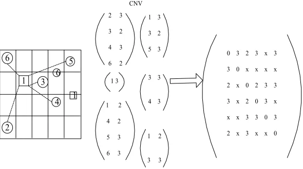
Step 1 is to quantify the distance according to the wireless radio frequency trans-ceiver wireless range R, and then, according to the node's quantization level and neighbor node response information, to prepare the node's Close-Neighbor Vector (CNV). This is shown in Figure 1:
Fig. 1. Distance quantization and CNV
In Step 2 for the node's CNVs, run the estimation algorithm according to these CNVs compiled into a connected matrix C, and then through the connected matrix C calculate the distance matrix D. This is shown in Figure 2.
1 6 1 6
3
2
4 5
2 3
3 2
4 3
6 2
1 3
3 2
5 3
1 2
4 2
5 3
6 3
3 3
4 3
1 2
3 3
0 3 2 3 x 3
3 0 x x x x
2 x 0 2 3 3
3 x 2 0 3 x
x x 3 3 0 3
2 x 3 x x 0 1 3
CNV
(2) Distributed arithmetic
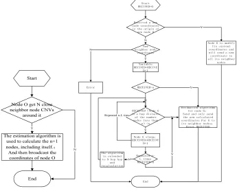
Assume that the network has a node that triggers the whole calculation process. The node acts as the origin of the role, also according to the CNV in and around it, the n neighbor node can calculate the coordinates of the neighbor nodes, where n is a threshold. Based on these CNVs, the origin node can calculate its coordinates in the local computation. Obviously, when the number of the threshold n is large enough, the calculated results will be accurate enough, but if the threshold n increases, more bandwidth will be consumed. Therefore, it is necessary to have a suitable number to compromise accuracy and bandwidth consumption. Through simulation analysis, it is revealed that the threshold n = 30 can obtain a good result. The flow of the distributed algorithm is shown in Figures 3, 4.
Node O get N close neighbor node CNVs
around it
Y
N
End Start
The estimation algorithm is used to calculate the n+1 nodes, including itself. And then broadcast the coordinates of node O
%#% ' ( !!!# %$ $%!# ! ( ! Y N !%!!* %$&## % !!# %$ ($ ( !!# %%! %$ !# !$ # Y $%%! !#% !# ! *$ % (&% !!# %$!#%! %$ !# !$-$% N !$"-( !# ! !!# % Y N ##!# +! !"$% !% &# !$$$% , Y
Repeated n-L tims N
!#% $)% %!!"!" #&%! "% %$ N Y
Fig. 3. Flow chart of the Fig. 4. Flow chart of general node algorithm origin node algorithm
3.2 Refinement algorithm
The previous stage just provides the initial values of the node position; in order to get a more accurate position value, the refinement step of the algorithm needs to be introduced, the purpose of which is the use of the estimated distances between the nodes to get more precise location values[8]. Refinement is performed in an ad-hoc
distance) is considered. The restrictions enable the refinement algorithm to be ex-tended to networks of arbitrary size and it does not support multi-hop routing (it re-quires only local radio) in the underlying network operation.
Refinement is a recursive algorithm; the nodes pass through a series of steps to up-date their location. At the beginning of each step, nodes broadcast their location es-timates and from their neighbor nodes receive their location value and the correspond-ing estimated distance. By solvcorrespond-ing the least square method and triangulation algo-rithm, they decide their new position. In most cases, the constraint imposed by the distance to the neighbor's position will force the new position closer to the true loca-tion of the node. After many cycles, the localoca-tion update becomes small, and the actu-arial method terminates and reports the final location.
The refinement algorithm has the advantage of being relatively simple. This is due to the limits on its use, especially under the premise that the refinement algorithm may not be able to achieve accurate results. Many factors will influence the refine-ment algorithm convergence and accuracy, so in the traditional refinerefine-ment algorithm an error threshold is introduced and the bad nodes of the control are eliminated.
4
Implementation of
EMDS-MAP(D) Algorithm
The algorithm is realized by the node class; the node function is mainly to receive messages, and local computation and messages are issued. Node algorithms are divid-ed into two kinds: anchor nodes and unknown nodes. To start the algorithm, all nodes will, by the interface StartMessage(), receive the MSG_STRAT’ message. As a mes-sage from the network class, it will initialize all anchor nodes and other variables, namely to the anchor node position which gives value. After that, all subsequent mes-sages will be received and processed through the Message() function, until it receives a MSG_STOP message, which is processed by StopMessage ().
4.1 Main variable in a class of nodes This: The ID value of the current node
Position: Node's current location of the valuation, the storage mode for floating point array and array size corresponding to the location of the dimension.
Status: State node status
At present, there are four kinds of states;
STATUS_ANCHOR: The node knows its location.
STATUS_UNKNOWN: The node failed to estimate its location. STATUS_POSITIONED: The node has already estimated its position.
STATUS_BAD: The node is either invalid or unable to locate the node (the specif-ic definition is different depending on the location algorithm).
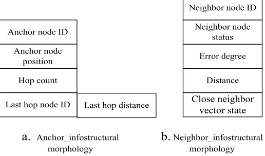
and the distance from the anchor node to the path of the current node on the last hop. If the current node is the anchor node, the first item of the list is stored in its own information, and is inserted into the list upon initialization.
Neighbors: Neighbor node information storage mode for the linked list. Each table entry contains neighbor node information, as shown in Figure 5 (b). The information includes the neighbor node ID, the neighbor node status, the neighbor node error degree , distance to the neighbor node, and CNV state indicates the neighbor node's neighbor vector state.
CNV_status: The nearest neighbor vector state of the node is a floating point array. It is a two-dimensional array, namely, the nodes of the ID and quantization levels.
Error: Error of node.
Refine count: The current node refinement times.
Anchor node ID
Last hop distance Last hop node ID
Hop count Anchor node
position
Close neighbor vector state
Distance Error degree Neighbor node
status Neighbor node ID
a.
Anchor_infostructuralmorphology
b.
Neighbor_infostructural morphology Fig. 5. The corresponding data items in the location algorithm4.2 Main message
... Anchor
node1 Number of anchor
nodes Source node ID
Package type
CNV Node position
estimation Forwarding node
hop count Source node ID
Package type
MSG_POSITION
Message packet MSG_ANCHOR Message packet
Anchor
node n Node 1 ... Node n
Node error
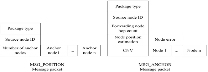
Fig. 6. Corresponding message packets in the localization algorithm
4.3 Computational cost
In the calculation of the distance measurement, the main calculation is focused on the generation of the distance quantization and the connected relation matrix. For a nodes, each node will perform the a times quantization, and note that in the last sec-tion, all the anchor nodes assumed can reach all the nodes, which is still set up here. After a times quantization, the a CNVs are calculated, and the connected relation matrix is generated.
In the refinement algorithm, each node performs the least squares method and gen-erates a new error matrix in each iteration. Assuming the algorithm after n circulation, the calculation of least squares method is D*(c-1)+(c-1)*(2*D+1)+(c-1)*2*(D+1) +D2*(c-1)+D3/3=(c-1)(5D+3)+(c-1)*D2+D3/3, where C is all nodes in the one-hop neighborhood, and the computation of each error matrix requires C additions and 1 division. The total number of calculations required for each node in the refinement algorithm is n[(c-1)(5D+3)+(c-1)*D2+D3/3+c+1].
4.4 Energy cost
BCt, BCr, and F are used to represent the transmission energy consumption, prima-ry energy consumption, and single calculation (flop) energy consumption (related to a specific system).
Measurement algorithm
Communication energy cost a*BCt+ac*BCr
Calculation energy cost a[1+(a-1)(D2+5D+3)+D3/3]*F Refinement algorithm
Communication energy cost n*BCt+nc*BCr
Calculation energy cost n[(c-1)(D2+5D+3)+D3/3+c+1]*F Total cost
Communication energy cost (a+n)*BCt+(ac+nc)*BCr
4.5 Algorithm complexity
Assuming the total number of nodes is n, the number of anchor nodes is m, for a n*n matrix, the time complexity of the measurement algorithm is O(e*n*logn), where e is the number of edges in the graph calculated according to the matrix. Each node in the distributed algorithm uses n auxiliary nodes and a three-dimensional embedding dimension at most, so the computational complexity of each node is O(e*n*logn+n2). The Dijkstra algorithm is used to calculate the shortest path distance matrix, the time complexity is O(n2). The time complexity of the multidimensional scaling algorithm is O(dn2), where d is the number of the embedding dimension. It uses m anchor nodes to calculate the relative coordinates to the absolute coordinates of the conversion parameters for the complexity of O (m3) and thecompletion of the relative coordi-nates to the absolute coordicoordi-nates for the complexity of O (n).
5
Simulation experiment
Design the EMDS-MAP(d) algorithm using MATLAB simulation, set the envi-ronment for the region of 100 x 100 randomly generated 200 nodes, and the nodes in a wireless communication radius of 10. In a network of 200 nodes, all data points are contained in more than 100 times the experimental results of the average value. In order to reduce the error of the distance between the simulation nodes, the distance value is subject to the standard distribution of the mean of the real distance.
In this paper, the simulation experiment is conducted under the condition of the distance measuring error being 2.5%. If the error range increases, the node localiza-tion accuracy will decrease, but the node localizalocaliza-tion accuracy will be improved if compared with the original algorithm. Due to the limitation of experimental condi-tions, if one wants to change the location error, one needs to build an experimental platform. But we will not elaborate on this, which is the next step.
In the simulation experiment, the "anchor node 5%" is the 5% of the total number of anchor nodes. The percentage of "unknown node localization" refers to the location accuracy of unknown nodes.
Defined mean error is defined as follows in Formula (7).
!""#" ! ! !!"#!!!!"#$! !
! !!"#!!!!"#$! ! !
!!!!!
!!! !!!!! ( 7)
Among them, n and a respectively represent the total number of sensors and the to-tal number of anchor nodes; R(d) represents the node's wireless communication radi-us. The lower the average error is, the better the method is.
(1) Error experiment
The two sets of experiments are in the error range of 2.5%, using the average error Formula (7) to calculate, select anchor node ratios of 5%, 10%, and 20%.
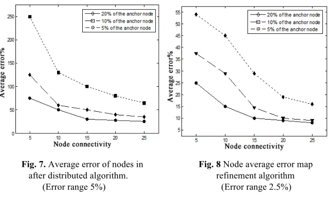
Fig. 7. Average error of nodes in Fig. 8 Node average error map after distributed algorithm. refinement algorithm
(Error range 5%) (Error range 2.5%)
In extreme cases, when the network's anchor nodes connectivity degree is very low, the algorithm error rate even reached 250%.
Figure 8 is the distributed algorithm refinement algorithm obtained by experiment. As shown in Figure 8, the curve shape and Figure 7 are similar, but it is evident that when the error degree greatly decreases, the in node connectivity is 5, and all three anchor node proportions of error are not more than 55%. If the connectivity degree and the proportion of anchor nodes are large, the node localization accuracy can ex-ceed 90%.
The experimental results of the analysis show, an improved algorithm for sparse anchor nodes and a low connectivity degree; the performance is not very good, but the refinement algorithm can greatly improve the localization accuracy.
(2) Location contrast experiment
The two sets of experiments are in the error range of 2.5%, and the anchor node ra-tio is 5%.
Figure 9 shows the percentage of the EMDS-MAP (D) algorithm in the distributed algorithm and refinement algorithm of the unknown node positioning. Experimental results further show that in low anchor node probability and sparse networks, there will be a large localization error. At the same time, we can clearly see a 5% anchor node; when the connected degree is large enough (at least more than 10), the position-ing of the unknown nodes' percentage continued in a relatively stable range.
Figure 10 shows the classic algorithm and EMDS-MAP (D) algorithm for the loca-tion of the unknown node percentage. The experimental results show that the differ-ence between the improved algorithm and the classical algorithm is obvious. In sparse networks, the localization performance of the improved algorithm is not as good as that of the classical algorithm, but when the node connectivity is greater than 10, the localization rate of the improved algorithm will be significantly higher than that of the classical algorithm.
6
Conclusion
In this paper, we design and implement a distributed localization algorithm EMDS-MAP (D) algorithm based on the MDS-EMDS-MAP. Experimental results show that in a high connectivity degree and a higher proportion of the anchor node, the node locali-zation accuracy of the EMDS-MAP (d) algorithm is higher than that of the classical algorithm. The introduction of the refinement algorithm can further improve the accu-racy of the node localization. Due to the algorithm's being calculated, steps are dis-persed in each node, thus reducing the computational complexity of the algorithm and thereby reducing the power consumption of the node battery operation and prolong the lifetime of the nodes.
7
Acknowledgment
This work was partially supported by National Nature Science Fund of China (NSFC)(Grant No.61403229, 61503213), Quzhou Science and Technology Project (2014Y006).
8
References
[1]Akyildiz I.F, Su W, Sankarasubramaniam Y., Cayirci E. (2002). A Survey on Sensor Net-works. IEEE Communications Magazine. 40(8):102-114 https://doi.org/10.1109/MCOM. 2002.1024422
[2]Lewis F.L. (2004). Wireless sensor networks. In D.J.Cook and S.K.Das, editors, Smart Environments: Technologies, Protocols, and Applications, New York, 35-64 https://doi.org/10.1002/047168659x.ch2
[3]Zhang L. (2008). Research on Distributed Localization Algorithm Based on wireless sen-sor networks. Hubei: Wuhan University of Technology, china,
[5]Zhang L., Han S.X., Fan W., Yang M.X. (2011). A Distributed MDS-MAP Algorithm for Wireless Sensor Networks[J]. Applied Mechanics and Materials. 52-54: 1626-1631 https://doi.org/10.4028/www.scientific.net/amm.52-54.1626
[6]Shang Y., Meng J., Shi H.C. (2004). A New Algorithm for Relative Localization in Wire-less Sensor Networks. In: Proceedings of the 18th International Parallel and Distributed Processing Symposium(IPDPS’04), 26-30+24
[7]Liu Y., Xing J.P. (2011). Three dimensional node localization algorithm in wireless sensor networks with random communication radius. Journal of sensing technology, 1(24): 88-92 [8]Wei Li Xiong, Tang Mengna, Xu Baoguo. (2011). A for wireless sensor network node
po-sitioning new method. Journal of sensors and increasing, 4(24): 576-580
[9]Liu H.B., Cui J.M., Dai H.J. (2011). Wireless sensor networks based on multi classifica-tion algorithm for wireless sensor networks. Sensing Technology, 5( 24) : 771-777 [10]Zhang S.P. (2010). Research on node localization algorithm in wireless sensor networks.
Wuhan: Huazhong University of Science and Technology
[11]Vidhya T.V., Raju G.S.N. (2015). Pattern Synthesis Using Modified Differential Evolution Algorithm. Modelling, Measurement and Control A. 88(1): 24-40
[12]Sandeep C.S., Sukesh K.A. (2015). A Review on the Early Diagnosis of Alzheimer’s Dis-ease (AD) Through Different Tests, Techniques and Databases. Modelling, Measurement and Control C. 76(1): 1-22
9
Authors
Lu Zhang received the B.Sc. degree from the Department of Computer Science and Technology, Zhengzhou University, China, in 2003 and the M.A.Sc. degrees from the Department of Computer Application, Wuhan University of Technology, China, in 2008. Now she is a lecturer in School of Electrical and Information Engi-neering, Quzhou University and is a doctoral candidate in School of Computer Sci-ence and Technology, Wuhan University of Technology.
Hailun Wang received the B.Sc. degree from the Department of Automation, Changchun University of Technology, China, in 2002 and the M.A.Sc. degrees from the Department of Electronic and Communication Engineering, Zhejiang University of Technology, China, in 2006. Now she is an associate professor in School of Elec-trical and Information Engineering, Quzhou University and is a doctoral candidate in Power electronics and power transmission, Shanghai Maritime University.
Zhiyong Hu received the B.Sc. degree from the electrical engineering and automa-tion,Tianjin University, China, in 2001 and the M.A.Sc. degrees from the flight vehicl e design, Harbin Institute of Technology, China, in 2006. Now he is a lecturer in Department of Radio Navigation, Dalian Air Force Sergeant School of Communi-cation.
Deyong Wang received the B.Sc. degree from the Department of mechanical en-gineering, Henan Polytechnic University, China, in 1992 and the M.A.Sc. degrees from the School of Software, XiDian University, China, in 2007. Now he is a profes-sor in school of Computer, Pingdingshan Industrial Collage of Technology and is a doctoral candidate in School of Resource and Environmental Sciences, Wuhan Uni-versity of Technology.