An Optimal Localization Algorithm of
Wireless Sensor Networks
https://doi.org/10.3991/ijoe.v14i01.8057
Chunxiang Wu
Guangzhou Institute of Technology, Guangzhou, China
Abstract—To overcome the low accuracy and high energy consumption of positioning algorithm in wireless sensor network, we proposed a optimization positioning based on algorithm neighborhood model. Based on the characteris-tics of the neighborhood model, the algorithm selects the best beacon node and calculates the proximity distance to transmit the distance information to the base station. The base station uses the MDS-MAP algorithm to determine the location of the unknown node. The simulation was conducted on NS-2 plat-form. The results show that the performance of the proposed algorithm was bet-ter than traditional optimization algorithms. Significant enhancement is ob-tained with the proposed algorithm in terms of node distance estimation error and position error.
Keywords—wireless sensor network positioning, neighboring degree, path op-timization
1
Introduction
In recent years, wireless sensor networks (WSN) are developing rapidly and can be widely used in monitoring the wide range of military, environmental, public housing, medical and so on application environment. Determining the location of events is a crucial issue in wireless sensor network applications, and it is meaningless if the sensed data had no location information. This requires the use of positioning mecha-nism and algorithm and only in this way can we obtain the position of nodes in wire-less sensor networks [1].
improved MDS-MAP algorithm to calculate the coordinates of unknown nodes, to determine whether the positioning effect meets the requirements of error.
2
State of art
In the range of positioning error, since no ranging method has quite low require-ment for the hardware, it is suitable for large-scale wireless sensor networks. Most of the existing non range location algorithms based on connectivity and hops are affect-ed by the uncertainty of hop distance, that is, all hops have the same distance [4-5]. The distance between the nodes is crucial to the positioning algorithm[6]. In this sec-tion, a method of density calculation distance based on nodes is proposed by studying the neighborhood model between nodes. The idea of the algorithm is to measure the proximity of nodes by using the number of common nodes of two neighboring nodes, and to calculate the relative distance of neighbor nodes. A routing protocol is built in so that the path from the node to the base station is the shortest[7-8]. The distance information of the nodes is stored in the neighbor list and sent to the base station, and the base station uses the improved MDS-MAP algorithm for the positioning. The positioning accuracy is judged, and the positioning node satisfying the error require-ment is added to the beacon node ranks.
3
System model
3.1 Network model
This paper studies a wide range of wireless sensor networks, including a large number of sensor nodes. The network model does the following assumptions:
All nodes are stationary and densely distributed after deployment, and the unique ID number is identified to each node in advance.
Due to the anisotropic and heterogeneous environment of the antenna, the sensor nodes have different perception ranges. It is assumed that the radius of beacon node is larger than that of unknown node.
There is at least one path between any two nodes to form a connected network, and all communication links between adjacent nodes are symmetric.
Assuming that the location region is approximately a rectangle, according to the optimal deployment model of the beacon, when the beacon node is located on the two long sides of the rectangle and symmetrically distributed, the positioning performance is the best [3].
3.2 Relevant definition
The degree of node: in the formed connection network, the average number of 1 hop neighbor nodes in the sensor node communication range is defined as the degree of node.
Distance between nodes: the distance between nodes is linear distance. Neighborhood density: the number of neighbor node in the node communication range is represented by !. r denotes the communication radius of node i, and Ni refers to the number of neighbor nodes of node i.
!
"
=
(1)4
Design of NDLA algorithm
4.1 Calculation of adjacent distance
Ni represents the neighbor node set of node i, and Ni is defined as Ni={j|j"i&dij#r},
where dij denotes the Euclidean distance between the node i and the node j, and r is
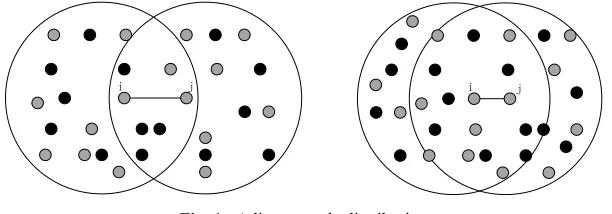
the communication radius. Obviously, this definition assumes a disk communication model, but such assumptions are uncommon in many range-free distance estimation or positioning schemes. Suppose that all nodes are similar, and the communication links among all neighbor nodes are uniform. All nodes have the same communication radius, and can form a connected network [5]. If two nodes were neighbor nodes, then the distance between them can be estimated. As shown in Figure 1, dij determines the
size of the overlap Areaij of the two nodes, and the larger dij is, the smaller Areaij will
be.
Fig. 1. Adjacent node distribution
According to the Monte Carlo algorithm, the area of the node communication range and the number of neighbor nodes can be approximately considered to be pro-portional relationship:
!
"
•
•
Nij refers to the number of overlapped region node, which can be obtained through
two nodes to exchange the neighbor information. $ is a correction parameter, and the error is decreased through the correction parameter. The distance from node i to the neighbor node j is defined as follows:
=
"
!
(3)In the network, nodes are randomly deployed. The number of node in the common parts and communication range is a random variable, and then
is a random variable. In that Nj is different from Ni, the distance from j to i and is also different. The average valueis regarded as the distance for neighbor nodes. The average value can distinguish the distance relationship be-tween two neighbor nodes, that is, the closer the distance is, the larger the value of Nijwill be, and the smaller the value of
. the further the distance is, the smaller the value of Nij, and the larger the value of . assuming that all nodes in thecommunication area of node i and node j are distributed uniformly, through numerical approximation method, it can be proved that the expectation of
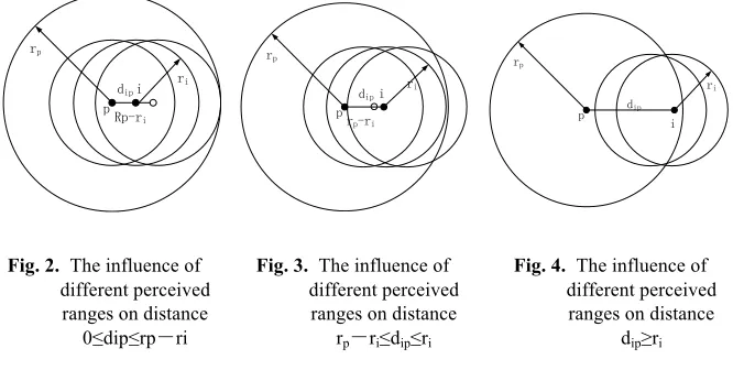
has linear relationship with dij [6].Whereas, in the actual application, due to the anisotropic and heterogeneous envi-ronment of the antenna, the perceive range of deployed node is different. Based on the calculation method of the same node radius, the cases of different radius is reasoned. The relationship between
and dij in some practical propagation models,such as the log quotient model is discussed. Assuming that the communication radius r of node follows Gaussian distribution, the average value r=70m and % is the standard deviation. As shown in figure 2 to figure 4, rp and ri represent the communication
radius of beacon node p and unknown node i, respectively. It is apparent that nodes that have larger perception range have more neighbor nodes, and the degree of nodes increases.
In figure 2, the communication area of node i is completely in the node p, and the area of cross region is &r2. The expected value of common neighbor node of node p
and node i is the same, and 0#dip#rpri. The more the neighbor node of a node is, the
more accurate the ratio relationship in (2) will be. As a result, the larger radius is selected for the calculation.
In figure 3, the area of cross region decreases with the increase of dis-tance.
and dip still meet the linear relationship and rpri#dip#ri.Fig. 2. The influence of different perceived ranges on distance
0#dip#rpri
Fig. 3. The influence of different perceived
ranges on distance rpri#dip#ri
Fig. 4. The influence of different perceived ranges on distance
dip'ri
4.2 Node position estimation
Large scale wireless sensor networks are constrained by computation and commu-nication. Sensors employ limited processors and micro controllers to reduce network costs. Unlike microprocessors, micro controllers are not able to run computationally intensive algorithms. Because of the limited energy and computing power of nodes, in addition, the power limited sensor cannot afford the power consumption when com-municating with remote nodes. The algorithm proposed in this paper divides the task, which is completed by the node and the base station together. The beacon nodes are arranged in the monitoring area in the semi-circular or round way. This deployment improves the positioning accuracy, and it is also convenient for the WSN being ap-plied in environmental monitoring, military reconnaissance, or target tracking [7]. A routing protocol is built in, and the path to the base station is created to transmit sens-ing data to the base station, reducsens-ing the energy consumption of nodes.
The unknown node transmits packets to the base station, and a packet has two parts: ID of the node and the distance information. The sensing node transmits the data to the nearest node and reaches the beacon node. As the sink node, the beacon node transmits the data to the base station. Recursively repeat this operation until all nodes transmit data in such a path. In fact, multi hop wireless sensor networks can be viewed as a graph G(V, E), where V represents a node set, |V| = n refers to the num-ber of nodes, and E indicates the edge set, that is the transmission distance between two hop neighbor nodes, and the beacon node is the root. The unknown node to select the nearest beacon node with the shortest distance is parent beacon node, as the short-est path [8]. This method is not only the shortshort-est path of the data to the base station, but also can ensure that the data is returned from the base station to the node because the connectivity between the nodes is bidirectional.
The sensor node finds the shortest path to the base station, and transfers its own ID, neighbor relationship and distance information to the base station. The base station uses the improved MDS-MAP algorithm to locate the unknown nodes. The base
tion establishes the initial distance matrix D(X) according to the extension graph G(V, E):
!
!
!
!
!
!
"
#
$
$
$
$
$
$
%
&
=
…
!
"
!
!
!
…
…
…
(4)The distance of non neighbor nodes in the matrix is unknown, labeled as -1, and the base station traversal matrix finds the line number and column number with the distance value of -1. Assuming that the distance values of row a and column C are -1, it suggests that the node a and the node c are non neighbor nodes, and the distance value is unknown. The distance estimation algorithm of non neighbor nodes runs on the base stations because the base station has high computing power and storage ener-gy. The minimum distance of the non neighbor nodes is calculated and put into the matrix.
The disadvantage of MDS-MAP algorithm is that the computational complexity is 0 (n3), and n represents the number of nodes in the network. The reason is that
MDS-MAP uses the shortest path algorithm to estimate the distance between any non neighbor nodes. In order to reduce the error of distance matrix, improvements of MDS-MAP are made: assuming that the network has 3 nodes A, B, and C, A and B, B and C are neighbor nodes, and A and C are non neighbor nodes, as shown in figure 3-4. The distance d1 between the node A and the node B is known, and the distance d2
between the node B and the node C is also known. Because the distance matrix needs the distance between each pair of nodes, the distance between the node A and the node C must be calculated. If A, B, and C are collinear, then the shortest path algo-rithm is used, and the distance between A and C is approximately a=d1+d2. If not
collinear, supposing that the node C is at the midpoint of arc C1 and C2, then the distance between A and C is:
=
+
!
•
•
(5)4.3 Determination of positioning error
By defining two constraint conditions, whether the unknown node positioning error meets the requirements is determined:
When the unknown node i is located, the estimated coordinate of the node i is used to calculate the distance to all the neighbor nodes, to judge the distance and the radius r. If it is larger than r, it suggests that the node i positioning deviation is large.
Calculate the estimated distance from the unknown node i to the adjacent beacon
the error requirements. And
!
is the average value of unknown node i and mneigh-bor beacon node error square.
After an unknown node is positioned, if it meets the above two conditions, it is considered that the unknown node is accurately positioned, and it becomes a new beacon node. Then, the original beacon nodes together participate in the positioning of other nodes. But the unknown node obtained by positioning algorithm has some errors relatively [9]. In order to reduce the superposition of the error, a credibility rel is given for each upgrade node. The value is proportional to the number k of beacon nodes around the upgrade nodes, and inversely proportional to the iteration times t and the proportional coefficient is µ:
=
µ
•
•
(6)With the gradual updating of the positioning process, the reliability of the newly generated beacon nodes is getting lower and lower. In the positioning process, the original beacon node is selected with priority to participate in the positioning. If the original beacon is less than 3, the reliability of the upgraded node is compared, and the nodes with high reliability are chosen to participate in the positioning.
5
Simulation experiment
In order to verify the performance and positioning accuracy of the proposed algo-rithm, the simulation test is carried out with NS-2. The proposed algorithm is com-pared with the improved DV-HOP positioning algorithm, the CMDS positioning algorithm, and the DV-CNED positioning algorithm.
The specific simulation parameters are as follows: MAC:MAC/802.11; simulation time: 6000s; receiving power consumption: 5m/w; Transmission power consumption: 150 m/w; Initial energy of unknown node: 2K/J; Initial energy of beacon node: 10K/J; Network region: 200(200; Total number of nodes: 100, 110, 120, 130, 140, and 150; Beacon node number: 10, 15, 20, 25, 30, and 35; Communication radius r (m): 50, 55, 60, 65, 70, and 75; simulation times: 20.
The simulation experiment evaluates the performance of the algorithm from two aspects: the node energy consumption and the node positioning error. It mainly tests the influence of the total number of nodes, the number of beacon nodes and the radius of communication on the positioning error.
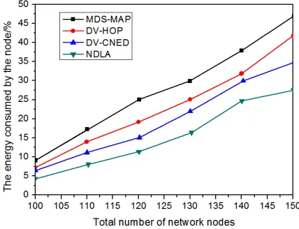
5.1 Energy consumption of nodes
the total number of network nodes, the energy consumption increases gradually. Be-cause the algorithm in this paper assigns the positioning tasks to the sensor nodes and the base stations. It can reduce the energy consumption and memory requirements of nodes, so the energy consumption is less than that of the other three algorithms. Alt-hough the data transmission of nodes need additional energy, the energy required for transmission is far less than the energy required for processing and computing data. At the same time, the improved MDS-MAP algorithm reduces the complexity of node localization, thus reducing the energy consumption of positioning calculation.
Fig. 5. Comparison of energy consumption of nodes
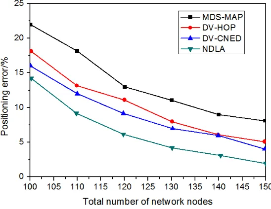
5.2 Node positioning error
Fig. 6. The Influence of Total Number of Nodes on Positioning Error
Fig. 7. The Influence of the Number of Beacon Nodes on the Positioning Error
6
Conclusion
Range free positioning algorithms are vulnerable to be affected by hop, node densi-ty, communication range and other factors. For solving high energy consumption and the positioning accuracy of the algorithm, the method to calculate the distance of the adjacent node according to the distribution model is put forward. In order to reduce the positioning error, the best beacon node is selected, to correct the distance error of beacon node, and the positioning task is sent to the base station to complete. The step and flow of localization algorithm based on proximity are introduced, and influence of communication radius, node density and the change of the number of beacon nodes on the algorithm positioning error is tested by NS-2 simulation. Compared with CMDS, improved DV-HOP and DV-CNED algorithm, the experiments show that the positioning performance is better than the other three algorithms in the parameters change. For wireless sensor networks, positioning accuracy, energy consumption and so on network overhead is contradictory and relevant to a certain extent. To obtain higher accuracy usually requires more overhead and it reduces the network lifetime. Lower precision makes the network efficiency become low. How to balance in these two aspects is determined according to the actual application.
7
References
[2]Colin, E. (2017). positioning in wireless sensor networks: A Dempster-Shafer evidence theoretical approach: Ad Hoc Networks, 54: 30-41. https://doi.org/10.1016/j.adhoc.2016. 09.020
[3]Shaimaa, M. M. (2017). Coverage in mobile wireless sensor networks (M-WSN): A sur-vey: Computer Communications, 110: 133-150. https://doi.org/10.1016/j.comcom.2017 .06.010
[4]Eliyeh, M. (2017). A robust method for underwater wireless sensor joint positioning and synchronization: Ocean Engineering, 137: 276-286. https://doi.org/10.1016/j.oceaneng. 2017.04.006
[5]Angel, S. (2016). Cooperative method for wireless sensor network positioning: Ad Hoc Networks, 2016: 61-72. https://doi.org/10.1016/j.adhoc.2016.01.003
[6]Avinash, M. (2017). A survey on energy efficient coverage protocols in wireless sensor networks: Journal of King Saud University - Computer and Information Sciences, 29(4): 428-448. https://doi.org/10.1016/j.jksuci.2016.08.001
[7]Slavisa, T. (2017). Distributed algorithm for target positioning in wireless sensor networks using RSS and AoA measurements: Pervasive and Mobile Computing, 37: 63-77.
https://doi.org/10.1016/j.pmcj.2016.09.013
[8]Samira, C. (2017). Distributed connectivity restoration in multichannel wireless sensor networks. 127: 282-295. https://doi.org/10.1016/j.comnet.2017.08.016
[9]Alessandro, R. (2013). An integrated system based on wireless sensor networks for patient monitoring, positioning and tracking: Ad Hoc Networks, 11(1): 39-53.
https://doi.org/10.1016/j.adhoc.2012.04.006
[10]Christian, E. Signaling game based strategy for secure positioning in wireless sensor net-works: Pervasive and Mobile Computing, 40: 611-627. https://doi.org/10.1016/j.pmcj. 2017.06.025
8
Authors
Chunxiang Wu is with Department of Information Engineering, Guangzhou Insti-tute of Technology, Guangzhou, 510075, China.