Mining and Learning in Sequential Data Streams: Interesting Correlations and Classification in Noisy Settings

(1)

PhD Dissertation

International Doctorate School in Information and Communication Technologies

DISI - University of Trento

Mining and Learning in Sequential Data Streams:

Interesting Correlations

and Classification in Noisy Settings

Katsiaryna Mirylenka

Advisor:

Prof. Themis Palpanas Paris Descartes University, France

Thesis Committee:

Prof. Alfons Kemper Technische Universit¨at M¨unchen, Germany

Prof. Minos Garofalakis Technical University of Crete, Greece

Prof. Yannis Velegrakis Universit`a degli Studi di Trento, Italy

(2)

Acknowledgements

My PhD benefited greatly from the contribution of many people who helped me to realize who I am and supported my work with excellent advice.

First of all, I would like to express deep gratitude to my scientific advisor Professor Themis Palpanas for the chance that he gave me, for countless life and professional lessons, and for his continuous help and support in different steps of my PhD life.

I also thank my teacher of mathematics Galina Yulianovna Guscha, and my first sci-entific advisor Elena Nikolaevna Orlova for showing me the beauty and the power of mathematical techniques.

I am very grateful to my internship mentors – Divesh Srivastava, Graham Cormode, and Vassilis Christophides – for the great opportunities they opened to me, and for the very useful insights on how to do research.

I thank my dearest friends and colleagues, who encouraged me during the years of my PhD, especially all the Belarusian community in Trento, and in particular our friends Volha and Aliaksandr.

(3)

Abstract

Sequential data streams describe a variety of real life processes: from sensor readings of natural phenomena to robotics, moving trajectories and network monitoring scenarios. An item in a sequential data stream often depends on its previous values, subsequent items being strongly correlated. In this thesis we address the problem of extracting the most significant sequential patterns from a data stream, with applications to real-time data summarization and classification and estimating generative models of the data.

The first contribution of this thesis is the notion of Conditional Heavy Hitters, which describes the items that are frequent conditionally – that is, within the context of their parent item. Conditional Heavy Hitters are useful in a variety of applications in sensor monitoring, analysis, Markov chain modeling, and more. We develop algorithms for effi-cient detection of Conditional Heavy Hitters depending on the characteristics of the data, and provide analytical quality guarantees for their performance. We also study the behav-ior of the proposed algorithms for different types of data and demonstrate the efficacy of our methods by experimental evaluation on several synthetic and real-world datasets.

The second contribution of the thesis is the extension of Conditional Heavy Hitters to patterns of variable order, which we formalize in the notion of Variable Order Conditional Heavy Hitters. The significance of the variable order patterns is measured in terms of high conditional and joint probability and their difference from the independent case in terms of statistical significance. The approximate online solution in the variable order case exploits lossless compression approaches. Facing the tradeoff between memory usage and accuracy of the pattern extraction, we introduce several online space pruning strategies and study their quality guarantees. The strategies can be chosen depending on the estimation objectives, such as maximizing the precision or recall of extracted significant patterns. The efficiency of our approach is experimentally evaluated on three real datasets.

(4)

Keywords

(5)

List of Tables

2.1 Lossless compression algorithms and their properties. . . 17

3.1 Main characteristics of the proposed algorithms . . . 34 3.2 Earth Mover’s Distance between the heatmaps of trajectories. . . 58 3.3 Mean Euclidean Distance (MED) and Misclassification Error (ME) of

dif-ferent prediction models for Taxicab dataset. . . 60

4.1 Characteristics of the online pruning strategies. . . 64 4.2 Comparison between the number of nodes in the full VMM trie and the

trie with only meaningful paths for different orders of VMM. . . 84 4.3 Average LogLoss of the fixed and variable order Markov Models. . . 85

5.1 The description of the datasets used. x1 is a number of classes, x2 is the

number of attributes (features), x3 is the number of instances, and x4 is

the intrinsic dimensionality of datasets. The sources of the datasets are given in the last column. . . 102 5.2 Dataset descriptions. x1 is the number of classes, x2 is the number of

instances, x3 is the autocorrelation lag, and x4 is the number of attributes

(features). The sources of the datasets are given in the last column. . . 105 5.3 Prediction error of linear regression models for non-sequential classifiers. . 115 5.4 Prediction error of linear regression models for sequential data. . . 117 5.5 Prediction error of logistic regression models for non-sequential data. . . . 119 5.6 Prediction error of logistic regression models for sequential data. . . 119 5.7 The values of three correlation coefficients between parameters of the dataset

and the parameters of the sigmoid. Non-sequential case. . . 120 5.8 Three correlation coefficients between parameters of the dataset and

(10)

(11)

List of Figures

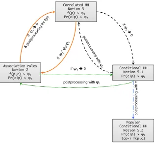
3.1 Comparison of various notions of interesting data stream elements. . . 32

3.2 Descriptive statistics for WorldCup’98 data. . . 44

3.3 Jaccard distance for top-τ conditional (CondHH) and simple (HH), CondHH and correlated(CorrHH) heavy hitters, and CondHH and Association Rules with red numbers correspond to r - the number of retrieved frequent item sets which are triples. . . 47

3.4 SparseHH accuracy for conditional heavy hitter recovery on Worldcup data under different reintroduction strategies. . . 48

3.5 Unique correlated and Conditional Heavy Hitters not detected by the other technique. . . 49

3.6 Accuracy on sparse synthetic data using SparseHH. . . 50

3.7 Precision (blue diamonds) and Recall (red squares) of SparseHH variations on sparse synthetic data as ρ varies. . . 51

3.8 Precision and Recall on the WorldCup data. . . 52

3.9 Accuracy as φ varies on Worldcup data . . . 52

3.10 Accuracy on sparse synthetic data as memory varies . . . 53

3.11 Time cost of algorithms on sparse synthetic data as memory varies . . . 55

3.12 Accuracy and timing results for algorithms on dense synthetic data . . . . 55

3.13 Accuracy on Taxicab data as memory varies . . . 56

3.14 Accuracy as φ varies on Taxicab data . . . 57

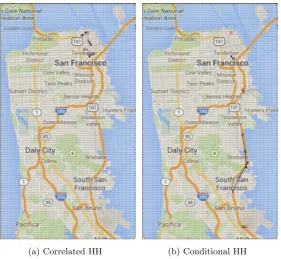
3.15 Heatmaps of trajectories modeled using exact transition probability matrix and recovered matrix based on Conditional Heavy Hitters. . . 57

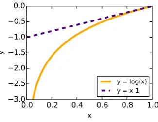
4.1 Approximating log(x) with x−1 forx close to 1. . . 68

4.2 Percentage of meaningful VOCHH candidates among all observed VOCHH candidates of a particular order. . . 79

(12)

4.4 Percentage of statistically significant VOCHH among all meaningful VOCHH of a particular order. Two statistical tests are used: “Freq test” – test of independence of the symbols of the full VOCHH sequence, and “CP test” – test of independence between the parent sequences and the child symbol. 81 4.5 Distribution of frequencies of the parent-child pairs for meaningful

statisti-cally significant VOCHH candidates with the frequency>1 for the Taxicab dataset. . . 82 4.6 Distribution of conditional probabilities of the parent-child pairs for

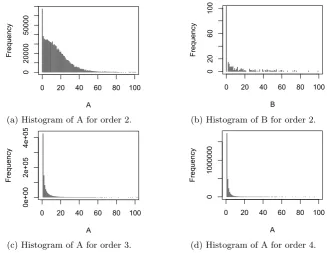
mean-ingful statistically significant VOCHH candidates with the frequency > 1 for the Taxicab dataset. . . 83 4.7 Distribution of the parametersA andB, which characterize the uniformity

of VMM for Taxicab dataset. . . 85 4.8 Average LogLoss of the fixed and variable order Markov Models and trie

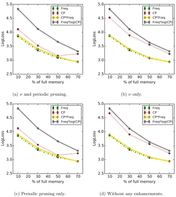
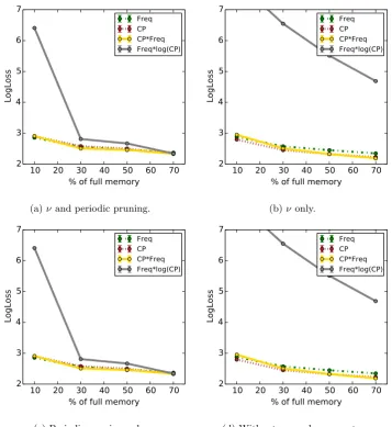
size of PPM-C for different maximum orders. . . 86 4.9 Average LogLoss for different algorithm variations for varying budget for

the BUWeb data. . . 87 4.10 Average LogLoss for different algorithm variations for varying budget for

the Taxicab data. . . 89 4.11 Validation of the approximate VOCHH algorithm for BUWeb data.

Mul-tiplication pruning. . . 90 4.12 Validation of VOCHH approximate algorithm for Taxicab data.

Multipli-cation pruning. . . 90 4.13 Validation of VOCHH approximate algorithm for TaxiCab data. Entropy

pruning. . . 91 4.14 Validation of VOCHH approximate algorithm for the WorldCup dataset.

Multiplication criterion. Maximum order 5. . . 91 4.15 Accuracies of VOCHH estimation for the BUWeb datasets for each order

separately. . . 92 4.16 The Mean Absolute Error of the conditional probabilities of VOCHH for

BUWeb dataset. . . 93 4.17 Top-τ accuracies of VOCHH estimation for WorldCup dataset for varying

values of τ. . . 93

5.1 Varying cparameter. c= 1 (left),c= 3 (right). Other parameters are the same: m= 0, M = 1, b= 2.5, d= 3. . . 97 5.2 Sigmoid function and points of interest. . . 98 5.3 Dataset grouping labels. . . 100 5.4 Distribution of the dataset characteristics. Real data: triangles, Artificial:

(13)

5.5 Distributions of the characteristics of sequential datasets. . . 104 5.6 Autocorrelation plot of the Pioneer gripper dataset. . . 104 5.7 Hidden Markov Model. X define the hidden states, while y are possible

observations, a – state transition probabilities, b – output probabilities. . . 106 5.8 Sigmoid CTF of the two settings of the HMM-based classification algorithm

for the “Robot walk 4” dataset. Green solid line: true measurements, dashed red line: estimated sigmoid. . . 108 5.9 Linear chain CRF architecture. . . 109 5.10 Sigmoid CTF of the two settings of CRF-based classification algorithm for

“Robot walk 4” dataset. Green solid line: true measurements, dashed red line: estimated sigmoid. . . 109 5.11 The architecture of RNN. . . 111 5.12 Sigmoid CTF of the two settings of the RNN-based classification algorithm

for the “Robot walk 4” dataset. Green solid line: true measurements, dashed red line: estimated sigmoid. . . 111 5.13 Sigmoid CTF of SMO and IBk algrorithms for “Wine” dataset. Green solid

line: True Measurements, dashed red line: estimated sigmoid. . . 112 5.14 Estimated SRF parameters per algorithm. X axis labels (left-to-right):

IBk, JRip, NB, NBTree, SMO. . . 113 5.15 SRF parameters per algorithm. X axis labels (left-to-right): CRF 1st

set-ting and 2nd setset-ting, HMM 1st setset-ting and 2nd setset-ting, RNN 1st setset-ting and 2nd setting. . . 114 5.16 Real and estimated values of the sigmoid parameters for non-sequential

classifiers. Real values: Black rectangles, Estimated values: circles, Gray zone: 95% prediction confidence interval. . . 116 5.17 Real and estimated values of the sigmoid parameters for sequential

(14)

(15)

Chapter 1

Introduction

In the last decades there has been a dramatic explosion in the availability of streaming measurements that naturally appear from different sources, such as sensor networks of human activities, position updates of moving objects in location-based services, mobile calls, climatological processes, financial transactions and others. Such data sources pro-duce billions of possibly noisy and temporally correlated values that arrive at a high rate, thus, making the tasks of pattern extraction, generative model estimation and sequential classification challenging.

In this chapter, we introduce three research directions that correspond to the problems of i) detecting interesting correlations, ii) estimating variable order generative models for sequential data streams, andiii) analyzing the performance of learning algorithms in noisy settings. Section 1.1 presents the general motivation for each direction. Then, in Section 1.2, we discuss the problem definitions and the contributions of this thesis. The structure of the thesis is given in Section 1.2.4. The publications based on the research made in this thesis are listed in Section 1.2.5.

1.1

Motivation

Due to its importance, the data stream model has received much attention in different research communities, such as data bases, data mining, networking, robotics and theory. There are many research problems that are addressed there, for example, data stream sum-marization [58], anomaly detection [21], data stream clustering [59] and classification [2]. In the majority of these works, adjacent observations of a data stream are treated as independent. In the recent works [35, 36] it has been demonstrated that it is beneficial to take into account the correlations between the neighboring observations for data modeling and related tasks that are based on similarity measurement among the parts of a data stream, such as pattern extraction, motif discovery, clustering and classification.

(16)

com-CHAPTER 1. INTRODUCTION

munities have extensively studied the behavior of classifiers in different settings[62, 112], the effect of labeling noise on the classification task is still an open problem.

1.1.1 Detecting Interesting Correlations in Fast Data Streams

Within applications that generate large quantities of data, it is often important to identify particular entities that are associated with a large fraction of the data items [34, 84]. For example, in a network setting, we often want to find which users are responsible for sending or receiving a large fraction of the traffic. In monitoring updates to a large database table, it is important to know which attribute values predominate, for query planning and approximate query answering purposes. This notion has been abstracted as the idea of “heavy hitters” or “frequent items”. Considerable effort has been spent on finding algorithms to track the heavy hitters under a variety of scenarios and data arrival models [7, 20, 25, 33, 78, 85, 88, 93].

However, the concept of heavy hitters can on occasion be quite a blunt one. Consider the network health monitoring scenario. It is well-known that in any measurement, there will be some destinations that are globally popular (search engines, social networks, video providers); likewise, so will be certain users (large organizations behind a single IP address, heavy downloaders and filesharers). As a result, tracking the heavy hitters within this data is not always informative, as they reveal only knowledge which is relatively slow changing, and not actionable. Rather, we would like to find which are sources or destinations that are significantly locally popular. That is, find those (source, destination) pairs where the destination is a heavy hitter amongst the connections of the same source.

Another application area is in security, in the intrusion detection domain. Here, a large number of different actions are observed, and the goal is to sift for unusual patterns of activity. The canonical approach is based around association rule and frequent itemset mining. These methods identify subsets of activities whose joint occurrence frequency exceeds some given threshold. While popular, this methodology has its limitations. The enormous search space implied by all possible combinations of actions typically requires a lengthy off-line search to identify the patterns of interest. While there are some on-line algorithms, these still require substantial resources to track sufficient statistics for the potentially frequent subsets. As a result, this kind of mining tends to be costly, and to deliver results significantly after the event.

(17)

1.1. MOTIVATION

meaningful definitions and a suite of algorithmic approaches to find them.

1.1.2 Estimating Variable Order Generative Models for Sequential Data Streams

Conditional Heavy Hitters, introduced in the previous section, correspond to sequential patterns of fixed order (length). If a data stream contains correlated subsequences of varying length, Conditional Heavy Hitters are not enough to capture the peculiarities of the data stream.

There have been few works devoted to online statistical and probabilistic modeling of data streams, where correlations among the values are taken into account, for ex-ample, estimation of regression models [57] and Hidden Markov Models (HMMs); but they reflect only linear dependency among the observations or only first order correla-tions [63, 118]. Currently, estimation of more sophisticated probabilistic models, such as high order HMMs, Conditional Random Fields (CRFs), or Variable Order Markov Models (VMMs) requires much space in order to keep the exponentially large number of parameters of high orders, which is infeasible for large alphabets and streaming settings. Conditional Heavy Hitters, described in Chapter 3, are capable of approximately estimat-ing the parameters of a high-order Markov chain with large alphabet, but keep the order of the model fixed.

In Chapter 4 we address the problem of online discovery of Variable Order Conditional Heavy Hitters (VOCHH) for data streams whose elements can be represented as symbols from large finite alphabets.

Specifically, we consider data that can be abstracted as pairs of temporally sorted symbols, which we refer to as a parent and a child. Parent consists of previously seen symbols, while a child usually corresponds to the most recent symbol. The fundamental concept of Conditional Heavy Hitters of variable order is to find those parent-child pairs, where the probability of the child is high, conditioned on the parent and the frequency of the parent-child pair is statistically significantly different from the i.i.d case of the distribution of the symbols. Variable order comes from the fact that parents can consist of variable number of symbols.

Streaming data from moving trajectories, sensors, web search, network monitoring, human activities, mobile wireless networks and text processing can naturally be mod-eled using variable order contexts, thus, they can be efficiently analyzed using VOCHH. VOCHH can be used to estimate the most important transition probabilities of the data generation models with markovian properties, such as Markov Models, HMMs, CRFs and others, in streaming environment. In other words, VOCHH extract the largest probabili-ties of moving from one state to another.

(18)

CHAPTER 1. INTRODUCTION

be stored is exponentially high. At the same time, to estimate all high order transition probabilities of a Markov Chain of a fixed order, much larger training datasets are needed. The variable order models estimate the parameters for only a small subset of meaningful contexts, thus, allocating space and using training datasets much more efficiently, which is crucial for streaming processing.

1.1.3 Analysis of Performance of Learning Algorithms in Noisy Settings

Conditional Heavy Hitters and VOCHH are useful for estimation of the generative model of the data stream in real time. The models can be exploited in the task of data stream classification. As streaming data often contain noise, it is important to study the behavior of classifiers in noisy settings.

Transforming vast amounts of collected – possibly noisy – data into useful information through the processes of clustering and classification has important applications in many domains. One example is preference detection of the customers for marketing. Another example is detection of negligent “providers” for Mechanical turk and reduction of their behavior on task results. The machine learning and data mining communities have ex-tensively studied the behavior of classifiers in different settings (e.g., [62, 112]), however, the effect of noise on the classification task is still an important and an open problem.

The importance of studying noisy data settings is augmented by the fact that noise is very common in a variety of large scale data sources, such as sensor networks and the Web, and Machine learning algorithms, both classical and developed for sequential data, perform differently in the settings with varying levels of labeling noise. Thus, there rises a need for a unified framework aimed at studying the behavior of learning algorithms in the presence of noise, depending on the specifics of each particular dataset.

In Chapter 5, we study the effect of training set label noise1 on a classification task. This type of noise is common in cases of concept drift, where a target concept shifts over time, rendering previous training instances obsolete. Essentially, in the case of concept drift, feature noise causes the labels of previous training instances to be out of date and, thus, equivalent to label noise. Drifting concepts appear in a variety of settings in the real world, such as the state of a free market, or the traits of the most viewed movie.

1.2

Problem Description and Contributions

1.2.1 Detecting Interesting Correlations in Fast Data Streams

In order to find interesting correlations, we model data that can be abstracted as pairs of items, which we refer to as parent and childitems. The central concept of Conditional Heavy Hitters is to find those parent-child pairs that are most frequent, relative to the

(19)

1.2. PROBLEM DESCRIPTION AND CONTRIBUTIONS

frequency of the parent. The reason for referring to such heavy hitters as “conditional” is by analogy to conditional probabilities: essentially, we seek children whose probability is high, conditioned on the parent. These should be distinct from the parent-child pairs which are overall most frequent, since these can be found by using existing heavy hitter algorithms. While this is a natural goal, it turns out that there are several ways to formalize this, which we discuss in more detail in Chapter 3. Thus, the first challenge is to formalize the notion of Conditional Heavy Hitters. As we consider streaming data that consists of symbols from possibly large alphabets, the second challenge is to accurately extract Conditional Heavy Hitters in real time with limited space budget. To this end, we developed several streaming algorithms that use pruning based on the value of the conditional probability. The core structure of the algorithms, which keeps estimated statistics about the frequencies of paren-child pairs, depends on the simple characteristics of data. The characteristics correspond to the expected size of possible parents that have at least one heavy hitter child. If the expected size of parents is small we call such a dataset “sparse”, otherwise, we refer to it as to a “dense” dataset.

Contributions. The main contributions of this research direction include:

• Definition of the concept of Conditional Heavy Hitters, which can be applied in a variety of settings;

• Theoretical and empirical comparison of Conditional Heavy Hitters with other no-tions of interesting elements studied in the data stream literature, such as frequent itemsets, association rules, and correlated heavy hitters;

• Development and description of several streaming algorithms for retrieving Condi-tional Heavy Hitters and analysis of their applicability for data with varying charac-teristics;

• The algorithms developed are evaluated on a mixture of real and synthetic datasets. We observe that certain algorithms can retrieve the conditional heavy hitters with high accuracy while retaining a compact amount of historical information. Different algorithms achieve the best results depending on simple characteristics of the data: essentially, whether the number of Conditional Heavy Hitters is comparable to the number of parents, or whether it is much lower.

1.2.2 Estimating Variable Order Generative Models for Sequential Data Streams

Studies [41, 74, 82, 104] show that for various domains, such as language modeling, cor-rection of corrupted text, speech recognition, machine translation, protein models and models for web page prediction, VMM provide better fit than fixed order models and use much less space, which is crucial to our problem of modeling data from large alphabets.

(20)

con-CHAPTER 1. INTRODUCTION

texts. This means that if the maximum order of the context is chosen, then, the fixed order model of this order leads to the smallest bias and the largest variance. The cause of the largest variance is the lack of evidence for estimating the parameters of the fixed-order model with enough confidence. Other words, fixed order model leads to the overfitting. On the other hand, using the smallest context information leads to underfitting, when bias is the largest and variance is the smallest. The main challenge of this work is to devise proper notion of variable order Conditional Heavy Hitters and develop online methods of their extraction in order to balance the bias-variance tradeoff in limited memory settings. To achieve this, we focus on the variable order modeling aimed at keeping all the impor-tant contexts that correspond to the significant dependencies of the data, and keeping the shortest possible contexts for the independent observations.

Our approach for VOCHH discovery exploits the variations of well known lossless compressionalgorithms [13] that are used for building an efficient representation of VMMs. Lossless algorithms with the best accuracy guarantees and at the same time the best performance originate in suffix trees or their analogs [22], [13]. After training they can be used for different purposes of data analysis:

1. extraction of essential connections between a symbol and a context – in order to find out the highest conditional probabilities of various orders.

2. forecasting – to predict future states of a data stream given a sequence of previous states;

3. similarity matching – to compare several parts of a data stream or several data streams based on their representation structures. This can be further used for clas-sification and clustering tasks.

Lossless compression algorithms have several limitations: tree structures keep the in-formation of all seen subsequences, thus, in case of large alphabets and, consequently, large number of states, the trees can grow up to the length of the stream and exceed memory budget. The algorithms that involve pruning, such as Probabilistic Suffix Trees, have running time quadratic in the length of the stream, thus making online usage im-possible. Other pruning strategies proposed in the literature are either too simplistic, for example, based on the frequency of a subsequence, or require much time to reconstruct the representation tree like in Probabilistic Suffix Trees.

(21)

1.2. PROBLEM DESCRIPTION AND CONTRIBUTIONS

Contributions. Main contributions of this thesis along this research direction include:

• Definition of the concept of Conditional Heavy Hitters of Variable Order.

• Several streaming algorithms for retrieving VOCHH.

• Analysis of the developed algorithms, including quality guarantees with regard to the VOCHH estimation.

• The developed algorithms are evaluated on three real-world datasets. We observe that the algorithms can retrieve VOCHH with high accuracy while using restricted memory budget.

1.2.3 Analysis of Performance of Learning Algorithms in Noisy Settings

Giannakopoulos and Palpanas [53] have shown that the performance2 of a classifier in the presence of noise can be effectively approximated by asigmoid function, which relates the signal-to-noise ratio in training data to the expected performance of the classifier. We call this fact the “Sigmoid Rule”. In Chaptercha:srf we examine how much added benefit we can derive from the sigmoid rule model, by studying and analyzing the parameters of the sigmoid in order to detect the influence of each parameter on the learner behavior. Based on the most prominent parameters, we define several dimensions characterizing the behavior of the algorithm, which can be used to construct criteria for the comparison of different learning algorithms. We name this set of dimensions the“Sigmoid Rule” Frame-work (SRF). The dimensions of the “sigmoid rule” are useful for comparing algorithms, and can take into account different requirements of the user. We also study, using SRF, how dataset attributes (i.e., the number of classes, features and instances and the fractal dimensionality [39] ) correlate with the expected performance of the classifiers in varying noise settings.

In this work we also show that the “Sigmoid Rule” is equally applicable to the problem of sequential classification, where classifiers of a different nature (for example, based on Hidden Markov Models) are considered. Sequential classifiers are useful for datasets where samples rely on causal phenomena, based on the sequence of appearance. We consider datasets where instances are the points of time series, causing the relationship between adjacent points. Using SRF, we additionally study the influence of the dataset characteristics on the performance of sequential classifiers. The dataset characteristics in this case are the number of classes, features and correlation order (a measure of how many recent instances strongly correlate with the next instance).

Contributions. In summary, we make the following contributions.

• We define a set of intuitive criteria based on the SRF that can be used to compare the behavior of learning algorithms in the presence of noise. This set of criteria provides both quantitative and qualitative support for learner selection in different settings.

(22)

CHAPTER 1. INTRODUCTION

• We demonstrate that there is a connection between the SRF dimensions and the characteristics of the underlying dataset, using both a correlation study and regres-sion modeling based on linear and logistic regresregres-sion. In both cases we discovered statistically significant relations between SRF dimensions and dataset characteristics. Our analysis shows that these relations are stronger for the sequential classifiers than for the non-sequential, traditional classifiers, where the instances are considered to be independent.

• Our results are based on an extensive experimental evaluation, using 10 synthetic and 31 real datasets from diverse domains. The heterogeneity of the dataset collection validates the general applicability of the SRF for both non-sequential and sequential learners.

1.2.4 Thesis Structure

The thesis contains the following chapters:

Chapter 2 surveys background and the related work relevant to the research directions of this thesis. In more detail, we discuss the specifics of streaming model, consider relevant notions of interesting patterns proposed in the literature, survey lossless compression algorithms and discuss the methods that are used for the analysis of classifiers in noisy settings.

Chapter 3 is devoted to the problem of Detecting Interesting Correlations in Fast Data Streams. It describes the notion of Conditional Heavy Hitters and developed algorithms together with the analysis of their quality guarantees, as well as the experimental evalu-ation of the algorithms.

Chapter 4 presents our results along the direction of Estimating Variable Order Genera-tive Models for Sequential Data Streams. We devise optimal pruning strategy to minimize LogLoss of the variable order model and describe its online variations. We also discuss the developed algorithms for VOCHH discovery and their quality guarantees. Finally, we experimentally evaluate the algorithms using three real datasets.

Chapter 5 contains the description of the Sigmoid Rule Framework, including the cri-teria that can be used to choose the optimal classifier in the noisy settings for a particular dataset. We also present the analysis of dependence of classifier’s performance on the dataset characteristics. The analysis is done for both classical and sequential classifiers.

Chapter 6 presents concluding remarks and directions of future work.

1.2.5 Publications

Research presented in this dissertation resulted in the following publications:

(23)

1.2. PROBLEM DESCRIPTION AND CONTRIBUTIONS

Comparison. Proceedings of the 2nd ACM SIGSPATIAL International Workshop on Querying and Mining Uncertain Spatio-Temporal Data. ACM, 2013: 8–15 (QUeST ’2011).

• [92] Katsiaryna Mirylenka, George Giannakopoulos Themis Palpanas. SRF: A Frame-work for the Study of Classifier Behavior under Training Set Mislabeling Noise. Advances in Knowledge Discovery and Data Mining. Lecture Notes in Computer Science. Springer Berlin Heidelberg, 2012. 109-121 (PAKDD’2012).

• [37] Michele Dallachiesa, Besmira Nushi, Katsiaryna Mirylenka and Themis Pal-panas. Uncertain Time-Series Similarity: Return to the Basics. Proc. VLDB En-dow. VLDB Endowment. 2012 (VLDB’2012).

• [90] Katsiaryna Mirylenka, Graham Cormode, Themis Palpanas and Divesh Srivas-tava. Finding Interesting Correlations with Conditional Heavy Hitters. Proceed-ing of IEEE 29th International Conference on Data EngineerProceed-ing(2013): 1069–1080 (ICDE’2013).

(24)

(25)

Chapter 2

Background and Related Work

In this thesis we address the problem of mining and learning in sequential data streams along the directions of finding important patterns of the fixed and variable order, and analysis of classifiers in noisy settings. We propose methods of finding important pat-terns and a framework for classifier analysis. In this chapter we provide the necessary background and related work for the formulated problems and the proposed methods. In Sections 2.1 we describe the data stream model. In Sections 2.2, 2.3 and 2.4 we consider relevant notions of interesting patterns proposed in the literature, survey lossless com-pression algorithms and discuss the methods that are used for the analysis of classifiers in noisy settings.

2.1

Data Streams and Their Specifics

The recent development of tools that generate and monitor data online has led to the necessity of processing of huge quantities of data in very short time. This gave rise to a new kind of data model that is called adata stream.

Data stream can be defined as an unbounded sequence (x1, x2, ..., xn, ...) that is indexed on the basis of the time of its arrival at the receiver. Babcock et al. [8] point out some fundamental properties of a data stream system such as:

(a) data elements arrive continuously, sometimes with a different rate;

(b) there is no limit on the total number of points in the data stream;

(c) once processed, the element of a data stream can not be retrieved unless it was explicitly stored in the memory;

(d) the amount of the available memory is less than the size of the data stream;

(26)

CHAPTER 2. BACKGROUND AND RELATED WORK

In other words, a data stream is an ordered sequence of elements that needs to be processed online because otherwise it will be lost.

2.2

Detecting Interesting Correlations in Fast Data Streams

The notions of heavy hitters and frequent itemsets have been heavily studied in the database and data mining literature. Interest in finding the heavy hitters in streams of data goes back to the early eighties [17, 93], where simple algorithms based on tracking items and counts were developed. Thanks to the interest in algorithms for streams of data, improved methods have been developed over the course of the last decade. These include variants of methods that track items and corresponding estimated counts [40, 85, 88], and randomized “sketch” methods, capable of handling negative weights [25, 33]. These methods can all provide the guarantee that, given a parameter, they can find all items in a stream of length n that occur more thanntimes, while maintaining a summary of size O(1/). Equivalently, they estimate the frequency of any given item with additive error n. For further details and empirical comparison of methods, see the surveys [34, 84].

The heavy hitters are a special case of frequent itemsets: they are the frequent 1-itemsets. Additionally, all larger frequent itemsets consist of subsets of the heavy hitters. There has been much work dedicated to finding frequent itemsets (and their variations) in the off-line setting, often starting from the Apriori [3] and FP-Tree algorithms [64]. These concepts have been adapted to work over streams of data, resulting in algorithms such as FUP [24], and FP-stream [55]. A limitation of finding frequent itemsets is that the number of possibly frequent itemsets can become very large, meaning that the algorithm either has to track information about many candidates, or else aggressively prune the retained data, and risk missing out on some frequent itemsets. In formalizing Conditional Heavy Hitters, one aim is to form a compromise between heavy hitters (which are simple and for which space/accuracy tradeoffs can be provided) and frequent itemsets (which are much more complex, and for which no tight space guarantees are provided). Additional background on itemset mining in streams is given by Yu and Chi [127].

(27)

2.3. ESTIMATING VARIABLE ORDER GENERATIVE MODELS FOR SEQUENTIAL DATA STREAMS

Our notion of Conditional Heavy Hitters is related to models of (temporal) correlation in data, as captured by Markov chains. That is, given a sequence of items, the kth order transition probabilities are defined as the (marginal) probability of seeing each character, given the history of thek prior characters. In our terminology, setting the child as the new character and the parent as the concatenation of the k previous characters means that finding the Conditional Heavy Hitters maps on to finding the high transition probabilities in this Markov chain. The importance of considering correlations has been recently motivated within several domains [35, 37, 80]. There has been much prior work on capturing correlations in data via different Markov-style models, such as homogeneous Markov chains of high order, hidden Markov Models [12], Bayesian networks [97] and others [80, 119]. However, fitting these increasingly complex models requires a lot of CPU and I/O time and multiple passes over the data, and hence it is infeasible to estimate them in a streaming setting. For example, the simple Mixture Transition Distribution [101] aims to approximate the transition probabilities with a smaller number of parameters, but requires multiple iterations over the data to do so. By focusing on the Conditional Heavy Hitters, we also identify a small number of parameters to describe the distribution, but can recover these efficiently in a single pass over the data.

Most related to this work is the paper of Lahiri and Tirthapura [77] which considers the problem of ‘correlated heavy hitters’ over a stream of tuples (a, b). Here, (a, b) is a correlated heavy hitter ifais a simple heavy hitter (frequency exceeds ψ) in a sequence of single-dimensional records andbis a heavy hitter in the subset of tuples wherea appears. We discuss the similarity and differences of this definition to Conditional Heavy Hitters in Sections 3.2 and 3.3.

2.3

Estimating Variable Order Generative Models for

Sequen-tial Data Streams

(28)

CHAPTER 2. BACKGROUND AND RELATED WORK

its derivatives PPM-C [94] and PPM* [28]. In this section we consider theoretical and empirical properties of these algorithms together with another non-stochastic popular lossless compression algorithm LZ78 [129]. We discuss the PPM algorithm in detail in Section 2.3.4 because we use it as a foundation for our methods of VOCHH discovery.

2.3.1 Online Compression Algorithms

There are several types of compression algorithms [22]: (a) lossy and lossless; (b) online and multiple-pass; (c) stochastic and Ziv-Lempel-like. As we are interested in efficient and accurate VOCHH estimation for large finite-alphabet sources in streaming settings we focus on lossless, online and stochastic algorithms. Due to the very large source al-phabets it is not feasible to keep the counts of all seen sequences in a tree. The least informative nodes and sequences should be pruned. Thus, eventually we cannot guar-antee lossless compression. On the other hand, we cannot use lossy algorithms as they are developed for particular domains such as image or video compression or even text compression where prior knowledge about the data source is heavily exploited [121]. Cur-rently, online stochastic modeling techniques arguably provide the best data compression among techniques known according to both theoretical and empirical studies [22], [13]. These results belong to the performance of the PPM family of techniques which we are going to discuss in more detail later in the chapter.

The work [13] surveys the most popular compression methods and evaluates the meth-ods by their prediction accuracy for three different datasets of sequential nature, namely english text, music and protein (amino-acid) sequence datasets. The methods estimate VMM from a sequence of observed states. They build a model, based on a tree or a collection of trees in a way that, when we look up a ”context” (preceding states), we get a prediction or a probability distribution for the next state.

General features of the compression algorithms according to Begleiter [13] are the following:

• A tree that is used to represent the estimated VMM is constructed during a training phase.

• Given the tree, conditional probabilities of any order (if the tree is not bounded) can be calculated. If the order is bounded and a query is longer than the maximum depth of the tree, there are several tricks to calculate the probability distribution, for example, the largest parent subsequence is used to estimate the probability of the sequence.

• The methods provide lossless compression of data. Having a good lossless algorithm, data series can be efficiently encoded with a small number of bits, proportional to the entropy of prediction, which also means high prediction quality of the model. Thus, lossless compression can be considered as summarizaion of the data series.

(29)

2.3. ESTIMATING VARIABLE ORDER GENERATIVE MODELS FOR SEQUENTIAL DATA STREAMS

uniformity of VMMs (in Section 4.1 we discussed uniform and nonuniform models where the variable length depends only on a context or on a full sequence consisting of a context and a symbol).

The algorithms that perform the best according to the study [13] are the following:

1. PPM-C – the Prediction by Partial Matching, Method C, proposed in [94].

2. For the protein classification problems the best algorithm is LZ-MS [96], which is a modification of the Lempel-Ziv compression algorithm LZ78 [129]. It is shown in the work [10] that the running time of LZ78 can be improved if it is represented via suffix tree.

These algorithms and their master algorithm – the general suffix tree algorithm [113] – together with their variations are described in Table 2.1. It is also shown in the study [83] that usage of the prefix and suffix structures is the most beneficial for sequential pattern mining.

In the description of the algorithms we use the following notation:

• Training dataset consists of n strings (or trajectories) of total length N;

• D – the maximum order of the model, which shows the maximum length of depen-dency among the neighboring observations. The order of the model corresponds to the length of the context or a parent that is used for modeling time correlations;

• m – the length of the query string 1, that is the string whose probability we need to find.

• z – the number of occurrences of this string in the tree,

• r – the number of resulting LZ78 factors for the corresponding algorithm.

• Σ – a finite alphabet defining the possible values of the sequence elements.

The full VOCHH-related notation is listed in Appendix A.3.

According to the comparison and accuracy results provided in [13] and [22], PPM-C is the best performer, while LZ78 and PST, in addition to the lower accuracy, have larger space and time requirements for the calculation of conditional probabilities.

VOCHH can be extracted using the tree structures obtained after training a lossless compression algorithm. Many lossless compression algorithms build either a suffix or a prefix tree (trie) in linear time, and can thus be used for real time applications, if space pruning is implemented efficiently.

(30)

CHAPTER 2. BACKGROUND AND RELATED WORK

2.3.2 Pruning

As mentioned above, in the case of large alphabets and bounded space, the main issue is to efficiently prune the nodes that are not promising in a sense that they have low potential to become Conditional Heavy Hitters. Pruning strategies are not naturally embedded into the lossless compression algorithms, although several pruning strategies, such asleast recently used or least frequently used, are described in the litereture. The most popular and the easiest strategy is to fully rebuild a tree when memory budget is spent [49]. One of the reason why full model reconstruction is preferred is that for other strategies there is a need to keep additional pointers to track the least recently/frequently used sequences.

Study of the VMM usage for predicting web pages navigation [41] introduces the confidence-based pruning, which checks if there is a difference in conditional probabil-ities of several children given a parent. If all possible children are equiprobable, it is safely assumed that elimination of such a parent will not change the model. This strategy is not useful in the case of very large alphabets as it is almost impossible to observe a parent with all possible states following it.

In the work [74], in which the back off model is used, the quality of a model after pruning is measured by the improved average KL divergence, which consists of the sum of terms:

d(yk, σ) = P rf ull[yk, σ] log

P rf ull[σ|yk]

P r[escape|yk_]_P

f ull[σ|yk−1]

for those sequences (yk, σ) that were not observed in a training set. σ is a symbol from Σ, and probabilities P rf ull[·] are defined by the suffix tree. The work [74] uses another kind of pruning strategy in order to minimize the improved KL divergence with the full model: it aims to remove those elements from the full model that have the lowest values of d(yk, σ). All the nodes with the lowest values of the criteria are successively removed until the tree reaches the predefined size. If the node is decided to be removed, all its successor nodes are also removed. Due to heavy computation this pruning strategy can only be used offline.

As VMMs of high orders have large number of parameters, all related works consider mainly offlinepruning strategies: when an exact model is already built (or all exact prob-abilities are estimated) some parts of the model or some probprob-abilities with the smallest impact on the model are discarded. Even strategies like “least frequently used” are usually assessed in the offline fashion, though they can be used online as well.

2.3.3 Probabilistic Suffix Trees versus PPM-C

(31)

2.3. ESTIMATING VARIABLE ORDER GENERATIVE MODELS FOR SEQUENTIAL DATA STREAMS T able 2.1: Los sless compression algorithms and their prop erties. # Name Main structure Running time Space Pruning Applications Real- time In teresting facts T raining Searc h requirmen ts Apriori Ap osteriori usage 1.0 Suffix trees suffix tree O ( n + N ) O ( m + z ) O ( N ) truncation: max string length is defined -space complexit y O ( min ( N | Σ | D + D n ) strings with c h aracte ris-tics that can b e expressed as a non-decreasing fu nc-tion, can b e p r u ned from the tree, without incre a s-ing space or time complex-it y , for example suffix fre-quency

text- editing, free-text searc

h,

compu- tational biology

y es, small al-phab ets all the algorithms b e-lo w are the v ariation of Suffix tr ees, also differ-en t PPM and LZ78 al-gorithms can b e imple-men ted via suffix tree structure 1.1 Coun t

suffix trees

suffix tree O ( n + N ) O ( m + z ) O ( N ) sp ecific to text, ex-ploit ling uisti cal fea-tures : regarding only the suffixes that are useful in a lin-guistic sense - syllab-ification, stemming, and non-w ord detec-tion text y es, small al-phab ets for frequency based pruning, strategies for probabilit y estima-tion: maxim um o v erlap (MO) an d others from w ork [66] can b e used 1.2 PST suffix tree + pruning dur-ing construc-tion O ( D · N 2) O ( D ) O ( D · N ),

though low

er than traditional case sym b ols are pruned if marginal probabil-it y ¡ threshold, ra-tio to the sequence with shorter suffix has comparable prob-abilit y no, due to quadratic time accuracy is no t v ery go o d, but when bac k-off mo d e l for zero-frequency prob lem is used, the p erformance is b etter (closer to PPM) [72] 2.0 PPM trie, for b ounded order mo del O ( N ) O ( | par ent | 2) O ( D · N ) frequency-based pruning, conditional probabilit y based pruning p ossible online text, DNA y es, small al-phab ets can b e represen ted as a suffix tree, b est p er-former 2.1 PPM* trie, with un-b ounded or-der mo del O ( N ) O ( | par ent | 2) O ( N ), m uc h

larger space require- men

ts than 2.0 no no text, DNA y es, small al-phab ets can b e represen ted as a suffix tree, un b ounded k eeps all information ab out the sequence, lin-ear in space, bad com-pression as k eeps ev ery-thing, o v erestimates lo-cal Mark o v mo del 2.2 PPMC trie with

inexact frequency coun

(32)

CHAPTER 2. BACKGROUND AND RELATED WORK

subclass of Probabilistic Finite Automata that is used to model transitions between the finite number of states). The PST algorithm has PAC-style performance guarantees [104]: for some small δ and it is proven that with the probability 1−δ the Kullback-Leibler divergence between a true and an estimated distributions, after normalization by the length of the string, is less than .

The PST algorithm is not a real time algorithm, as it first extracts all the subsequences bounded by the maximal order D with their exact counts, then calculates the maximal likelihood estimates for all transitional probabilities, and finally uses some refinements to keep only significant ones. These refinements can be seen as offline pruning strategies. Each candidate subsequence (y, x), which corresponds to a new node or a sequence of nodes, is examined for two conditions:

1. joint probability of the context and the symbol should be larger than the predefined threshold. This threshold can be converted to a frequency threshold;

2. the context y is meaningful if there is a symbol σ such that P(σ|y)> threshold; 3. the contextycontributes additional information for predictingσrelative to its longest

suffixy0 (if y= (x1, x2, ..., xk) then its longest suffixy0 = (x2, x3..., xk)). This means that the ratio of their conditional probabilities is significantly different from one:

P(σ|y)

P(σ|y0₎ ≥1 +ε or

P(σ|y)

P(σ|y0₎ ≤

1

1 +ε, (2.1)

where ε >0.

All the thresholds depend on,δ, the size of the alphabet, and length of the strings used for training. The procedure for building PST has quadratic time complexity (O(D∗N2), and the space complexityO(D∗N), whereN is the length of the training data, andO(D) is the time required to find P(σ|y).

Several additional offline pruning criteria for PST were used in the work [82]. The first two pruning strategies from PST are adopted as they are, while the last strategy that checks if a node brings additional information compared to its parent is reformulated. In the previous work [104], difference from a parent suffix is checked separately for each symbol using the equation 2.1, while in the paper [82] the difference is checked using Kullback-Leibler divergence between distributions ˆP(·|σy) and ˆP(·|y). If the difference is smaller than a threshold, then the node is pruned. This criterion is efficient only for small alphabets, as the Kullback-Leibler divergence is calculated when distribution over all the symbols is defined.

(33)

2.3. ESTIMATING VARIABLE ORDER GENERATIVE MODELS FOR SEQUENTIAL DATA STREAMS

testing fixed order Markov Chains of different orders, then model with the minimal AIC is considered as a starting point for further pruning. On the next level, each parent-child pair is considered in order to choose the model based on either the parent or the son. According to the results on the protein data [82], using the AIC criterion results in the significantly smaller size of the PST, as well as the improved quality of prediction. AIC still needs offline processing due to the multiple passes over the data.

In most of the lossless compression algorithms that are used for prediction2 so called “zero-frequency problem” is faced. Zero-frequency problem corresponds to those cases where the sequence for which the probability should be predicted has not been seen in the training dataset. To address zero-frequency problem (P[σ|y] = 0), the PST approach uses a small, user-defined probability to be assigned to it: P[σ|y] = pmin. This part is additional and it does not participate in PAC learning guarantees.

Interestingly, though the PST algorithm has good theoretical properties, it did not perform well in the empirical studies [13], [72], which compared different lossless compres-sion algorithms for the purpose of building VMM models. In fact, PST was not among the three best performers.

Prediction by Partial Matching. PPM and especially its variation PPM-C perform the best. PPM-based algorithms can be represented as a suffix tree [22] and PST and PPM keep essentially the same information as PST, but in different data structures. The main difference between these two algorithms is the implementation of zero-frequency problem for sequences that have not been seen in a training set. While PST uses minimal probability threshold, PPM uses a complex mechanism of escape and exclusion, which has very good empirical performance, despite having no theoretical guarantees. This escape mechanism in also called back-off technique. The technique can be formulated as Equation 2.3.4, where P r(escape|y) is different for different implementations, but they depend on the number of symbols seen aftery – Σy, a context y and probabilities of seen symbols.

The back-off technique helps to define a model completely on demand when an estima-tion of the probability of an unseen sequence is needed. ParameterP r(escape|s) is needed in order to get distributions to sum to unity. Thus, in PPM algorithms the probability of unobserved symbols is not fixed and depends on the number of observed symbols and the frequency of a context, while in PST this minimal probability is the same for any context. It is demonstrated in the work [72] that usage of similar mechanism for PST improved its performance greatly.

As we focus on the streaming settings, we build our approach based on the best per-forming PPM algorithm, as it has training time complexityO(n) and has the potential for online pruning. The main challenge of our approach is to tackle PPM space complexity O(D*n), which is infeasible for the streams with large alphabets. For prediction we use

(34)

CHAPTER 2. BACKGROUND AND RELATED WORK

the best performing back-off model implemented in PPM-C version of PPM algorithm which is described below.

2.3.4 Prediction by Partial Marching

In this section we describe in more detail the PPM compression algorithm and its PPM-C variation that we will use as the basis of VOCHH estimation. The main parts of the algorithm are the following [13]:

Input:

(1)D– the maximal order of dependency (maximum context of VOCHH parent), and, at the same time, the maximal depth of the tree which contains the model information;

(2)Escape andexclusion mechanisms, which are used to solve the zero-frequency prob-lem for the contexts which were not seen during training. There are various PPM al-gorithms depending on different escape and exclusion mechanisms. In general, escape mechanism works as follows, for all the contexts y with the order k ≤ D we need to allocate a certain probability mass ˆPk(escape|y) for all symbols that did not appear after the context y. The remaining probability mass 1−Pkˆ (escape|y) is shared among symbols with non-zero frequencies. The probability mass allocation differentiates PPM algorithms, nevertheless, all algorithms follow the recursive equation following [13]:

ˆ

P(x|y) =

( ˆ

Pk(x|y),if F r(y, x)6= 0

ˆ

Pk(escape|y)·P rˆ (x|y0), otherwise.

(2.2)

The exclusion mechanism is based on the fact that probabilities of observed symbols given a context can be estimated more accurately if they are calculated using just the observed set of symbols rather than all possible symbols.

Learning phase:

PPM algorithm constructs a trieT based on the data stream s= (x1, x2, ..., xN). Each node in T corresponds to a symbol from the alphabet Σ and has a counter. The depth of the trie T is bounded by the order D and is less or equal to D+ 1. The root node of T corresponds to an empty symbol. The algorithm incrementally parses the training sequence, one symbol at a time. Each symbol and its context of the length up to Ddefine a path in T. The counter of any node with the corresponding path (y, x) is F r(y, x), where y is the parent or the context of a path, and x is the child or the last symbol; The learning phase requires linear time O(N) to be finished. The space required for the worst case trie is O(D·N).

There are several types of trie updates that are used in PPM variations:

(35)

2.3. ESTIMATING VARIABLE ORDER GENERATIVE MODELS FOR SEQUENTIAL DATA STREAMS

2. Update Exclusion (used in PPM-C) – only the frequencies that correspond to the maximum suffix-tree frontier are updated. The frequencies are updated if it is a new symbol of a parent, or it is a maximum frontier (length) symbol;

3. MaxOrderUpdates – counts are updated only when a new symbol is a maximum order state. For the descendants all the counts are smaller than real, similarly to the previous case.

The last two types of updates lead to faster training, but make the trie inconsistent for pruning, as all the non-leaf nodes have counts smaller than their real frequencies.

As in the best-performer – PPM-C algorithm – no pruning was implemented, during the training phase not all counts of the nodes corresponding to a training path were updated, only the leaf nodes have valid up-to-date counts. As we would like to implement further pruning, we use the standard PPM full update procedure.

Testing/prediction phase:

When a trie T is built (the building can be continuous and a testing sequence can be included in the trie) it encodes the probability distribution of variable order of the training dataset. Probabilities ˆP(x|y), |y| ≤ D can be calculated by traversing the trie along the longest suffix ofy, denoted as y0, such that (y0, x) are fully contained in T as a path from the root to a leaf. Then the counters along the path are used to calculate the probabilities using the following equations:

ˆ

Pk(x|y) =

F r(y, x)

|Σy|+ P

x00_∈_Σ

yF r(y, x

00₎, if x∈Σy; (2.3)

ˆ

Pk(escape|y) =

|Σy|

|Σy|+P_x00_∈_Σ

yF r(y, x

00₎, otherwise, (2.4)

where|y|=k, Σy is the set of symbols seen so far in the context of y. The straightforward computation of ˆP(x|y) using T requires O(|y|2_{) time [13]. This escape mechanism is}

considered among the best [13] in practice. At the same time, according to Witten and Bell [122] there is no principle justification among different escape mechanisms.

2.3.5 Model Validation: LogLoss

Here we discuss the goodness of fit methods for estimated VMM models, which are used to see how well the built model describes initial data. As we already mentioned before, the compression algorithms for VMM estimation are validated using LogLoss on the testing dataset [13]. LogLoss is defined as follows:

l( ˆP , xk) = −1

k k X

i=1

log ˆP(xi|x1, x2, ...., xi−1). (2.5)

(36)

CHAPTER 2. BACKGROUND AND RELATED WORK

LogLoss computation there is no need to assess the full probability distribution from the trie including the cases that are not encoded in the trie. The conditional probability is estimated only for the current testing sequence. LogLoss which is also called cross-entopy loss or logistic regression loss is defined on the estimated probabilities, and is widely used to evaluate probability outputs of prediction and classification tasks, for example, it is used as one of the loss optimization functions by the winners of the KDD Cup Orange Challenge in 2009 [42] and KDD Cup 2004 [116] and for model evaluation in the work [128]. The authors of the work [107] show that if models are well calibrated, LogLoss is the highest-performing selection metric if little data is available for model selection.

There is a direct connection between LogLoss, lossless compression, and entropy. The quantity −log₂P r(xt|x1, ..., xt−1) is called “self-information”, it is the compression or

code length of symbol xt and it is measured in bits per symbol. The expected value of self-information is the entropy. So, LogLoss is the average of the self-information for each symbol in a test sequence. The average LogLoss is the average compression rate of a sequence, given the estimated distribution _P [13]. The equivalence of the LogLoss minimization and compression is shown in the works [103], [102]. This validation fits the case where we are interested in the prediction of the next points given the context.

Sometimes, for the model validation, similarity measures between several distributions, such as Kullback-Leibler divergence or Jensen-Shannon divergence, are used. For their calculation it is required to estimate all the probabilities of the model, even those probabil-ities which are not estimated because not all possible contexts are seen during the training phase. Since we are interested in detecting only strong correlations , the measures above cannot do us justice, since they value the detection of weak correlations equally. As we would like to concentrate only on the largest conditional probabilities given the variable order contexts, validation metrics similar to logloss are more preferable.

2.3.6 Comparison with Other Notions of Interesting Correlations

Among the notions that describe elements of interest in the streaming data series are Heavy Hitters, Frequent Itemsets, Correlated Heavy Hitters, Association Rules and others that are compared with the Conditional Heavy Hitters of the fixed order and discussed in Section 3.3. Association Rules is the closest notion to the Conditional Heavy Hitters of Variable Order, as both of them focus on the pairs that have high frequency and high conditional probability of occurrence. At the same time, a parent in the pair has variable length.

The main differences between Association Rules and VOCHH are the following: 1. In Association Rule world there is no single global sequence, the patterns are

(37)

2.4. ANALYSIS OF PERFORMANCE OF LEARNING ALGORITHMS IN NOISY SETTINGS

2. Sequential Association Rules do not try to find Markov style patterns, though there is sequentiality there. In general, Association Rules are used to find the correlation phe-nomena among the items, but they are not devised to make direct predictions [106]. 3. There may be time gaps in the timestamps of items in the rule. In one transaction there is no sequential relationship between the items. In contrast, the VOCHH approach assumes that all the observations are sequential.

Studies devoted to the discovery of Association Rules can be divided into four main branches:

(a) Original Association rules, which operate through the thresholds on support and confidence [3], as discussed in Section 3.3;

(b)Streaming algorithms for the online discovery of Association Rules [67];

(c) Sequential Association Rules, that take into account order of the itemsets [65, 106]. The order might be with the gaps in the timestamps, thus the parts of the rule may happen not in the adjacent transactions;

(d)Association Rules with statistical foundation, where statistical significance of the rule or the set of rules is taken into account [61, 73].

Our VOCHH approach can be seen as a product of all the branches of Association Rules but with Markov sequentiality and a single generative model.

2.4

Analysis of Performance of Learning Algorithms in Noisy

Settings

Since 1984, when Valiant published his theory of learnable [114], setting the basis of Probably Approximately Correct (PAC) learning, numerous different machine learning algorithms and classification problems have been devised and studied in the machine learning community. Given the variety of existing learning algorithms, researchers are often interested in obtaining the best algorithm for their particular tasks. The algorithm selection is considered to be a part of the meta-learning domain [56].

According to the No-Free-Lunch theorems (NFL) described in the work [125] and proven in the works [123, 124], there is no overall best classification algorithm, given the fact that all algorithms have equal performance on average over all datasets. Nevertheless, we are usually interested in applying machine learning algorithms to a specific dataset with certain characteristics, in which case we are not limited by the NFL theorems. As mentioned in the work [5], the results of NFL theorems hint at comparing different classification algorithms on the basis of dataset characteristics, which is the aim of our work in this research direction.

(38)

CHAPTER 2. BACKGROUND AND RELATED WORK

the authors compared algorithms on a large number of datasets, using measures of per-formance that take into account the distribution of the classes, which is a characteristic of a dataset. The Area Under the receiver operating Curve (AUC) is another measure used to assess machine learning algorithms and to divide them into groups of classifiers that have statistically significant difference in performance [18]. In all the above studies, the analysis of performance has been applied for the datasets without noise, while we study the behavior of classification algorithms in noisy settings. In our study we use the fact shown by G. Giannakopoulos and T. Palpanas [53, 54] about concept drift, which illustrates that a sigmoid function can accurately describe performance in the presence of varying levels of label noise in the training set. In an early influential work [75], the problem of concept attainment in the presence of noise was also indicated and studied in the STAGGER system. In this thesis, we analytically study the sigmoid function to determine the set of parameters that can be used to support the selection of the learner in different noisy classification settings.

The behavior of machine learning classifiers in the presence of noise is also considered in the work [70]. The artificial datasets used for classification were created on the basis of predefined linear and nonlinear regression models, and noise was injected in the features, instead of the class labels as in our case. Noisy models of non-markovian processes using reinforcement learning algorithms and the methods of temporal difference are analyzed in the paper [98]. In the work [26], the authors examine multiple-instance induction of rules for different noise models. There are also theoretical studies on regression algorithms for noisy data [111] and works on denoising, like [81], where a wavelet-based noise removal technique was shown to increase the efficiency of four learners. Both noise-related studies [81, 111] dealt with noise in the attributes. However, we study label-related noise and do not consider a specific noise model, which is a different problem. The label-related noise corresponds mostly to the concept drift scenario, as was also discussed in the introduc-tion 1.2.3.

(39)

2.4. ANALYSIS OF PERFORMANCE OF LEARNING ALGORITHMS IN NOISY SETTINGS

we also apply this framework to sequential classifiers, which were not considered in above studies.

(40)

(41)

Chapter 3

Streaming Conditional Heavy

Hitters

In this chapter we tackle the problem of finding interesting correlations in data streams. We have introduced the notion of Conditional Heavy Hitters in Section 4.5.1. In this Chapter, first, we discuss the motivating applications of Conditional Heavy Hitters in Section 3.1 and describe necessary preliminaries in Section 4.5.1. Then, in Section 3.3, we discuss similarities and differences of Conditional Heavy Hitters with other notions of interesting elements studied in the data stream literature, such as frequent itemsets, association rules, and correlated heavy hitters. In Section 3.4 we present several streaming algorithms for detecting Conditional Heavy Hitters and analyze their applicability for data with varying characteristics. In Section 3.5 the developed algorithms are evaluated on a mixture of real and synthetic datasets. The algorithms can detect Conditional Heavy Hitters with high accuracy while retaining a small amount of historical information. Furthermore, these algorithms are able to process the streams arriving at a high speed. In Section 3.5.6 we also show the ability of extracted Conditional Heavy Hitters to accurately estimate the Markov Model of moving trajectories.

The work presented in this chapter has been published as a conference paper [90] and as a journal paper [89].

3.1