Open Access
Research article
Fine structure of the low-frequency spectra of heart rate and blood
pressure
Tom A Kuusela*
1, Timo J Kaila
2,3and Mika Kähönen
4Address: 1Department of Physics, University of Turku, 20014 Turku, Finland, 2Department of Clinical Pharmacology, Tampere University
Hospital, 33521 Tampere, Finland, 3Tampere University, 33014 Tampere, Finland and 4Department of Clinical Physiology, Tampere University
Hospital, 33521 Tampere, Finland
Email: Tom A Kuusela* - tom.kuusela@utu.if; Timo J Kaila - timo.kaila@kuusamo.fi; Mika Kähönen - mika.kahonen@uta.fi * Corresponding author
Abstract
Background: The aim of this study was to explore the principal frequency components of the heart rate and blood pressure variability in the low frequency (LF) and very low frequency (VLF) band. The spectral composition of the R–R interval (RRI) and systolic arterial blood pressure (SAP) in the frequency range below 0.15 Hz were carefully analyzed using three different spectral methods: Fast Fourier transform (FFT), Wigner-Ville distribution (WVD), and autoregression (AR). All spectral methods were used to create time–frequency plots to uncover the principal spectral components that are least dependent on time. The accurate frequencies of these components were calculated from the pole decomposition of the AR spectral density after determining the optimal model order – the most crucial factor when using this method – with the help of FFT and WVD methods.
Results: Spectral analysis of the RRI and SAP of 12 healthy subjects revealed that there are always at least three spectral components below 0.15 Hz. The three principal frequency components are 0.026 ± 0.003 (mean ± SD) Hz, 0.076 ± 0.012 Hz, and 0.117 ± 0.016 Hz. These principal components vary only slightly over time. FFT-based coherence and phase-function analysis suggests that the second and third components are related to the baroreflex control of blood pressure, since the phase difference between SAP and RRI was negative and almost constant, whereas the origin of the first component is different since no clear SAP–RRI phase relationship was found.
Conclusion: The above data indicate that spontaneous fluctuations in heart rate and blood pressure within the standard low-frequency range of 0.04–0.15 Hz typically occur at two frequency components rather than only at one as widely believed, and these components are not harmonically related. This new observation in humans can help explain divergent results in the literature concerning spontaneous low-frequency oscillations. It also raises methodological and computational questions regarding the usability and validity of the low-frequency spectral band when estimating sympathetic activity and baroreflex gain.
Background
The existence of spontaneous fluctuations in heart rate and blood pressure has been known for a long time in
modern cardiovascular physiology [1]. The spectral analy-sis of heart rate and blood pressure is a widely used non-invasive technique to assess autonomic indexes of neural Published: 13 October 2003
BMC Physiology 2003, 3:11
Received: 21 May 2003 Accepted: 13 October 2003
This article is available from: http://www.biomedcentral.com/1472-6793/3/11
cardiac control [2–4]. Such analyses typically focus on three separate frequency bands: a high-frequency (HF) band, a low-frequency (LF) band, and a very-low-fre-quency (VLF) band; the standard frevery-low-fre-quency ranges of these bands are usually >0.15 Hz, 0.04–0.15 Hz, and 0.003–0.04 Hz, respectively. The selection of these bands reflects the assumption that each is related to a certain car-diovascular mechanism [5–9]. In normal conditions the presence of a spectral peak in the HF band of RRI spec-trum is closely related to respiration and is attributed to vagal mechanisms. Another frequency peak in RRI spec-trum can be found within the LF band, which is attributed predominantly to sympathetic mechanisms but partially also to vagal mechanisms. It is often reported that this fre-quency peak is centered on 0.1 Hz (also called Mayer waves), but the frequency of this oscillation and the underlying mechanisms are still uncertain. Oscillations at frequencies in the VLF band are often related to the vaso-motor tone of thermoregulation or to the dynamics of hormonal systems, but the origin and frequency of the oscillations in this band are still unknown.
It is widely believed that a single peak in the entire spec-trum reflects a specific mechanism of cardiovascular con-trol which can be quantitatively measured by determining the area under that peak, i.e., the corresponding spectral power. However, there are many studies suggesting either that a single peak can originate from a complex set of var-ious control mechanisms, or that a single control mecha-nism can produce several peaks [8,10,11]. Additionally, it is known that both the amplitude and frequency of the oscillations within VLF, LF, and HF bands can vary with the physiological conditions [12–14].
This study investigated the details of the spectra of the R– R interval (RRI) and systolic arterial blood pressure (SAP) in the LF and VLF frequency ranges in order to characterize the principal frequency components in healthy humans. Three spectral methods based on totally different mathe-matical approaches were used; the use of several methods is crucial to validation of the results. We have not explored possible mechanisms behind each frequency component, but we do discuss the phase conditions between RRI and SAP in the VLF and LF bands.
Methods
Subjects and study protocol
A total of 12 healthy subjects (age 20–26 years) partici-pated in the study. The study protocol was approved by the ethics committee of the Tampere University Hospital. The actual protocol consists of several different phases, but only two of them were used in this study. In the first phase (lasting 12 minutes), the subjects were studied whilst breathing spontaneously. After this phase the spec-trum of the respiration flow signal was calculated and the
peak frequency was determined. In the second phase (last-ing 12 minutes), the subjects were studied us(last-ing metro-nome-controlled breathing where the breathing frequency was adjusted to the value of the peak frequency of the respiration flow from the first phase. This arrange-ment guaranteed that in the second phase all subjects could breath at their natural breathing frequency so that the breathing frequency did not vary significantly. The spontaneous breathing frequency varied from 0.12 Hz to 0.25 Hz. Before the first phase there was 15 minutes adap-tation time to stabilize the hemodynamics, and there was a 5-minute rest period between the first and second phases. In all recordings the subjects were in supine posi-tion. Since the subjects were forced to follow the metro-nome sound it was possible to verify that they were not asleep.
Data acquisition
The following data were measured: ECG (Rigel 302 Cardi-oscope), continuous noninvasive blood pressure from the left middle finger (2300 BP Monitor, Ohmeda Inc., USA), pulmonary air flow (M909, Medikro Oy, Finland), expira-tion CO2 and O2 concentrations by capnometer (Datex Normocap, Datex Inc., USA), and oxygen saturation at the left ear lobe (Datex Satlite, Datex Inc. USA). All signals were digitized at a sampling rate of 200 Hz (WinAcq data acquisition system, Absolute Aliens Oy, Finland). The RRI time series were generated by detecting the R peaks of the ECG signal, and the SAP and diastolic pressure time series were generated by finding the corresponding beat-to-beat minimum and maximum on the blood-pressure signal within each RRI. All data analyses were performed with WinCPRS software (Absolute Aliens Oy, Finland).
Spectral analysis
The choice of spectral methods used in this study was crit-ical to the detection of any fine structure in the RRI and SAP spectrum within the LF range below 0.15 Hz. There are two main factors that must be considered carefully. First, in spectral analysis the frequency resolution is higher when longer time series are used, but only if the system under study is stationary over the time interval of the analysis, and in the present study we cannot make any
short-term spectra, and search for patterns that can be found on all of them. We have done this by calculating the spectra using a sliding time window of reasonably short duration and a time step that is much smaller than the window width. Since it is rather unlikely that there are sudden or abrupt changes in the heart-rate or blood-pres-sure regulation system, especially when the subjects are studied whilst supine, we can assume that RRI and SAP spectra vary only slowly. When tracking the position of the dominant frequency components we can easily recog-nize the fundamental modes since the corresponding spectral peaks will appear as continuous paths on the time–frequency plots.
We applied three methods to the spectral analysis of RRI and SAP time series: Fast Fourier Transform (FFT), autore-gression model (AR), and Wigner-Ville distribution (WVD). We selected these methods because they are based on totally different mathematical approaches and there-fore their combined use increases the likelihood of vali-dating our results. Detailed description of each of these spectral methods can be found on Appendix (see Addi-tional file: 1). AR method is most suitable for searching the principal frequency components since the spectrum can be easily decomposed using pole-expansion of the spectrum. In contrast, with FFT or WVD method it is diffi-cult to determine accurately the positions of the spectral peaks. However, the use of AR method is also problematic since the essential parameter of it, the optimal model order, is difficult to determine. Therefore we have used non-parametric FFT and WVD methods to help us for finding the best model order: the model order of the AR spectrum was adjusted in such a manner that the overall shape of the spectrum resembles FFT and WVD spectra. FFT and WVD spectra have typically reasonably high spec-tral resolution in the low frequency range but poor statis-tical relevance. The latter one can be improved by smoothing the spectra but then we decrease frequency res-olution. This unavoidable trade-off between statistical rel-evance and resolution complicates detecting spectral peaks reliably: spectra can include spurious features. However, since FFT and WVD spectra are computed using different mathematical approach it is very unlikely that these features appear simultaneously on both spectra, and therefore the combined used of FFT and WVD to resolve the optimal AR model order is crucial.
Results
A typical spectral analysis of the RRI of one subject is pre-sented in Fig. 1. The time–frequency plots (upper panels) were generated using three different methods: Fast Fourier transform (FFT), Wigner-Ville distribution (WVD), and autoregression (AR). The AR method has been used with two models: one of order 12 and the other of order 20. All methods are capable of distinguishing the respiration
component, which in this case is located at 0.15 Hz. Below this respiration frequency the nonparametric meth-ods – FFT and WVD – reveal at least two distinct compo-nents that appear in the figure as continuous red paths. With the FFT method, the paths are not very clear because of the limited frequency resolution. In the WVD plot the components are separated much better but the back-ground of the spectrum is contaminated by mixing of the main components (chessboard-type pattern), as explained in Appendix (see Additional file: 1). With the parametric AR method, the appearance of the spectrum depends heavily on the model order. When using the model order determined by Akaike's information crite-rion (AIC; 12 in this specific case), the spectrum is strongly smoothed and only one component can be seen below the respiration frequency (AR(12) in Fig. 1). When the model order is increased to 20, two separate LF com-ponents appear (AR(20) in Fig. 1). To show the differ-ences more clearly, in the lower panels of Fig. 1 we show cross-sections of the time–frequency plots at certain moments of time (marked with the white dashed lines). Both FFT and WVD spectra exhibit two peaks, at 0.06 Hz and 0.09 Hz, and perhaps also another two around 0.02 Hz. In the AR(12) spectrum there is only one wide spectral peak visible, but in the AR(20) spectrum there are two dis-tinct peaks at the same positions as in the FFT and WVD spectra, and a third lower one around 0.02 Hz. These results clearly show that AR spectral methods, as com-monly applied (i.e. with a relatively low model order), are unable to reflect the real frequency content of a signal; this leads to oversmoothed spectral profiles and to overmode-ling the actual variability. It should be noted that in the FFT and WVD spectral densities the height of each spectral peak corresponds directly to the spectral power, whereas in the AR spectrum density the height of the peak is pro-portional to the square of the power (the area under the peak is proportional to the power). Therefore, the differ-ences in the heights of the peaks in the AR(20) spectrum are much higher that in the FFT and WVD spectra.
analysis for all 12 subjects are presented in Fig. 2. The res-piration was controlled by a metronome, whose the
fre-quency was close to the normal supine respiratory frequency of each subject in order to avoid any physiolog-Time–frequency plots of the R–R interval
Figure 1
The main spectral peaks of the R–R interval Figure 2
ical stress produced by an unnatural respiration rhythm. This frequency component on the time–frequency plots is almost a straight line indicating a near constant frequency and its power is also highest (red or white path). In all cases there are three or four components below the respi-ration frequency, except for subject F whose respirespi-ration frequency was very low. In most cases the frequencies of these components are also quite constant over time. In only a few subjects did the number of the components vary; this was due to either the model order being too low or to real changes in the dynamics of the heart-rate control system. It should be noted that in all plots there is a spec-tral component around 0.025 Hz, which does not change significantly over time.
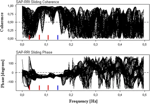
We also analyzed SAP in a similar manner, one example of which is presented in Fig. 3. The subject was the same
as for Figs. 1 and 2A. It can be clearly seen that the spectral components closely resemble those for the RRI. This sim-ilarity was also observed for the other subjects and there-fore we do not present the analysis results from them. To investigate the mutual character of the RRI and SAP we calculated the FFT-based coherence and phase between the RRI and SAP as a function of frequency and time using sliding time windows. The coherence and phase for the example subject in Fig. 1 are displayed in Fig. 4. To show the time-independent features clearly, the coherence and phase from all time windows are superimposed. The mean principal frequencies found from Fig. 2A are marked with red horizontal bars. Above the respiration frequency of 0.15 Hz, the coherence wanders between 0 and 1. Coherence values close to 1 in this frequency range indicate that there are momentary spurious oscillations or noise in RRI and SAP which temporarily oscillate coher-ently with a highly variable mutual phase difference. However, these oscillations are not physiologically important since their spectral powers are negligible. In contrast, the coherence is constantly high and the phase is almost constant at the respiration frequency of 0.15 Hz and around the spectral peaks at 0.07 Hz and 0.11 Hz (-50 to -30 degrees). However, around the spectral peak of 0.026 Hz the coherence and phase vary continuously with time. The results were very similar in all the other subjects.
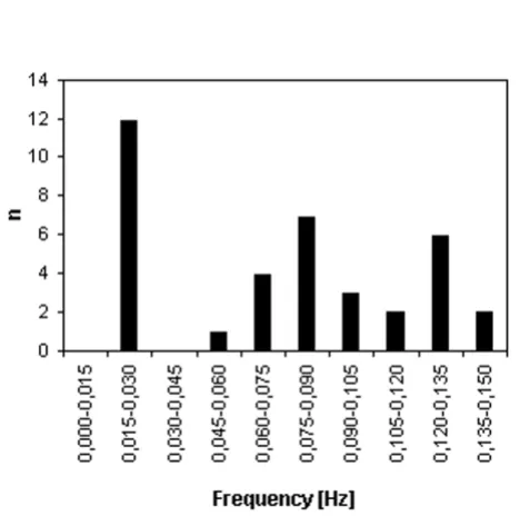
In order to estimate quantitatively the frequencies of the spectral components we first calculated the mean quency of each component below the respiration fre-quency for each subject (Table 1). We then calculated the averaged frequency of the first, second, and third compo-nents (starting from the lowest frequency component) over all subjects for which the components were available. The true first spectral component was always at zero fre-quency, but we excluded this because it corresponds to the uninteresting constant (or very slowly changing) part of the signal. The results are shown in Fig. 5. The average fre-quencies were 0.026 ± 0.003 Hz for the first component, 0.076 ± 0.012 Hz for the second component, and 0.119 ± 0.018 Hz for the third component. According to the standard t-test for independent samples, the averaged fre-quencies of each component were found to be different with a very high probability: p < 10-7 when comparing the first and second components, and p < 10-5 when compar-ing the second and third components. The distribution of frequencies is shown in Fig. 6, in which the frequency scale is divided into 10 equal bins. In all 12 subjects one frequency component was found in the frequency range 0.015–0.030 Hz, in seven subjects a component was present at 0.075–0.090 Hz, and in six subjects a compo-nent was present at 0.120–0.135 Hz.
To characterize more precisely the nature of each three principal frequency component we computed the Spectral analysis of the systolic blood pressure
Figure 3
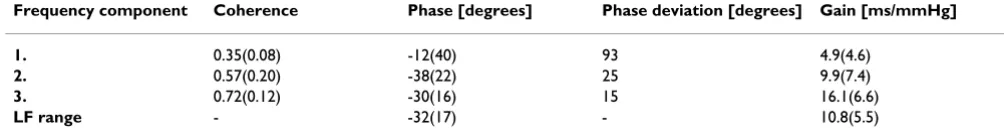
coherence, phase difference, deviation of the phase differ-ence and the gain between RRI and SAP for each subject at those frequencies found on Table 1. Analysis was done using the sliding FFT method with the same parameters as described previously, and all values were averaged over sliding segments. The mean results over 12 subjects are presented in Table 2. The coherence of the 2nd and espe-cially the 3rd frequency component is rather high (clearly above 0.5) indicating that corresponding oscillations in RRI and SAP are reasonably well correlated. In the case of the 1st frequency component the coherence is low (well below 0.5), and obviously oscillations in RRI and SAP at this frequency range are practically independent. The phase difference of the 2nd and 3rd component is clearly negative which can be interpreted as a sign that changes in SAP precede changes in RRI. The phase deviation
(deviation of the phase from segment to segment) of the 2nd and 3rd component is quite small, i.e. the phase is rather constant in time. The phase of the 1st component is also slightly negative but it is merely artificial result since the phase deviation is very large: the phase wanders freely in time. In fact the phase typically has all values from -180 to +180 degrees (the distribution of phase values is flat), and thus the large deviation cannot be explained by abrupt jumps from -180 to +180, as it would be possible if the phase difference between RRI and SAP were close to 180 degrees. All these observations are also visible in the example case of Fig. 4: the phase curves in the lower panel are tightly bundled at the 2nd and 3rd frequency compo-nents but not at the first component. The gain between RRI and SAP based on the transfer function approach seems to be lowest for the 1st component and highest for
The mutual coherence and phase of the RRI and SAP Figure 4
the 3rd component. Since the coherence related to the 1st component is low and the phase is not constant in time the corresponding gain value has very limited relevance. We have also computed the phase and gain in the LF band
in the normal way using only one segment covering the whole data (the last row in Table 2). The phase and gain were averaged over those frequency values where the coherence was higher than 0.5. This is the method, which is usually used when baroreflex sensitivity is estimated from spontaneous fluctuations of RRI and SAP. The phase angle is close to one of 3rd component but the gain is, in contrast, close to one of the 2nd component.
Discussion
Our main findings are as follows: (1) below 0.15 Hz there were at least three distinct peaks in both RRI and SAP spec-tra; (2) principal spectral components around the fre-quencies of 0.026 Hz, 0.076 Hz, and 0.119 Hz were found in all subjects; (3) the lowest spectral peak around 0.026 Hz was remarkably similar in all subjects and it did not vary over time; (4) the frequency of the other two main peaks clearly varied over time, but only slightly; and (5) the phase difference between the SAP and RRI was clearly negative and almost constant over time and the coherence was high in the case of the two highest frequency compo-nents, but in the case of the first component the phase and coherence did not exhibit stable characteristics.
Our approach to combine three different spectral meth-ods proved to be successful. AR method has superior frequency resolution if the model order is properly set, and the principal spectrum components can be easily computed. Commonly used information criteria to esti-mate the model order are inadequate, as we demonstrated in this study. In the most cases WVD spectra was useful for searching the optimal model order of AR spectra but sometimes we needed also FFT method to recognize the main features of spectra. Since the frequencies of the 2nd and 3rd principal components are not constant it is not possible to capture them using only single data segment, thus spectra should be computed as a function of time to uncover these components.
The presence of spectral components around 0.026 Hz in both RRI and SAP data is well known, and are widely believed to be related to the dynamics of thermoregula-tory processes [9]. However, the precise frequency of these oscillations has not been reported previously. In our study this oscillation mode was found in all subjects over a remarkably narrow frequency range. The corresponding period of about 39 s could, in principle, be an artifact of our analysis, such as being generated by the specific width of the time window used in our computations. To check this we also performed the analyses using considerably shorter and longer sliding windows, and found that this had no significant effect on the frequency. Since the coherence and especially phase between the SAP and RRI at this frequency varied over time, it is unlikely that this oscillation is a part of the blood-pressure regulation Mean and standard deviations of the frequencies of the first
spectral components Figure 5
Mean and standard deviations of the frequencies of the first spectral components. The mean frequency of the first three components in the LF range calculated over 12 subjects. Standard deviations are marked with vertical bars.
Distribution of the spectral components Figure 6
system, so it can be regarded as a secondary effect of some other mechanisms.
The existence of two or more distinct oscillatory compo-nents in the LF band was a striking observation. In the literature there are no specific reports of multiple spectral components in this frequency band in humans. In most cases the explanation is very simple: overall spectral power has been used as a measure of sympathetic activity, and detailed spectral composition has not been the target of the studies. It is very difficult to distinguish close spectral peaks using FFT analysis when sliding time win-dows are not used. Previous studies that have used AR modeling employed model orders that were too low to allow close peaks to be discriminated, as we have demon-strated. However, in animal studies there are some inter-esting reports on the presence of two spectral peaks within the LF band. Cevese et al. [15] investigated spontaneous fluctuations in heart rate and blood pressure in anesthe-tized dogs with the left iliac vascular bed mechanically uncoupled from the central circulation. They found indi-vidual peaks in RRI and SAP spectra at 0.03–0.07 Hz and at 0.12–0.17 Hz, and in some cases there was
simultaneously a peak in both frequency ranges. They suggested that the simultaneous peaks are simple har-monics of each other and that there is a unique causal mechanism behind this phenomenon. However, careful inspection of their data does not support this conclusion. In our data the two spectral peaks were not simple har-monics. Another interesting observation on oscillations well below 0.1 Hz has been reported recently [16]. In that human study alpha-blockade intervention produced a new spectral peak in some subjects centered at 0.04–0.05 Hz during which the "normal" peak around 0.1 Hz disap-peared. It is unclear whether this new spectral peak is asso-ciated with our findings since the phase difference between SAP and RRI at 0.04 Hz was reported to be -73 to -169 degrees, which is much more negative than our observations at 0.076 Hz. However, that study demon-strated that the spectral composition of RRI and SAP is not necessarily constant in all conditions. It should be noticed that spectral peaks well below 0.1 Hz have been reported in humans also in normal physiological conditions. Espe-cially with very elderly people the LF peak can shift signif-icantly towards lower frequencies [14,17] but, however, coexistence of two or more clear peaks on this frequency
Table 1: Principal frequency components of the R–R interval. Mean frequencies of the first three spectral components of the R–R interval for frequencies below 0.15 Hz.
Subject f1 [Hz] f2 [Hz] f3 [Hz]
A 0.026 0.069 0.102
B 0.028 0.073 0.122
C 0.027 0.076 0.122
D 0.022 0.055 0.086
E 0.024 0.062 0.099
F 0.026 0.072
-G 0.031 0.081 0.116
H 0.028 0.097 0.135
I 0.025 0.095 0.137
J 0.028 0.079 0.129
K 0.025 0.086 0.125
L 0.020 0.073 0.117
Table 2: Coherence, phase and gain between RRI and SAP. The mean RRI-SAP coherence, mutual phase difference, deviation of the phase difference and transfer function gain for each principal frequency component below 0.15 Hz (computed by the sliding FFT analysis) and for the LF frequency band (computed withing the LF band using a single data segment and coherence>0.5 condition). Each value is the mean(SD) over 12 subjects.
Frequency component Coherence Phase [degrees] Phase deviation [degrees] Gain [ms/mmHg]
1. 0.35(0.08) -12(40) 93 4.9(4.6)
2. 0.57(0.20) -38(22) 25 9.9(7.4)
3. 0.72(0.12) -30(16) 15 16.1(6.6)
region has not been reported previously. Since all subjects in our study were young and almost equal in age we can-not make any conclusions on the age dependence of the components.
One possible explanation of our findings is that the sepa-rate peaks were somehow produced by the respiratory component, either directly as subharmonics or by mixing with other components. These mechanisms would be possible if the system was highly nonlinear, but this is not very likely since in our experiments the respiration fre-quency was fixed by an external metronome and was dif-ferent for all subjects, and despite this we found two separate peaks both within a relatively narrow frequency range.
It should be noted that there are no a priori physiological conditions or requirements for only one spectral peak to be found within the LF band. Although the origin of LF rhythms in blood pressure and heart rate is still mostly unknown, two theories – the feedback theory and the cen-tral theory – have been considered the most probable. Both theories can support the existence of several spectral components in the LF band. Our findings do not elucidate a valid underlying mechanism, but they do suggest that the underlying system is more complex than commonly believed. Since the mutual coherence is high and the phase angle is clearly negative for both components, we cannot exclude the possibility that they are generated by baroreflex-mediated control. The diverse results in litera-ture on the frequency of oscillations of RRI and SAP in the LF band and the corresponding baroreflex-related latency times can be simply reflections on the fact that there exist two distinct component: sometimes the first one can be more dominant, sometimes another one. Thus the exist-ence of two simultaneous well-determined oscillations in the LF band gives rise to an important question about whether we can simply use the spectral power to quantita-tively estimate sympathetic activity or the transfer-func-tion approach to measure baroreflex gain. Our results indicate that the phase differences and gains between RRI and SAP related to two principal frequency components are significantly different. Phase and gain values com-puted by the commonly used method, i.e. applying anal-ysis on a single long data segment, seem to be approximately average (perhaps weighted by coherence) of ones of the separate components. Therefore currently used spectral method can be basically valid but the relia-bility and reproducirelia-bility can be rather poor since we don't know how various physiological situations, age of the subject and other factors modulate these two compo-nents. Our results clearly indicate that more detailed anal-ysis should be used when using spectral measures to estimate sympathetic activity and baroreflex sensitivity.
Conclusion
The data provided here indicate that the standard LF range of 0.04–0.15 Hz contains two frequency components, not one as widely believed, and that these components are not harmonically related. This new observation in humans can help explain divergent results in the literature con-cerning spontaneous LF oscillations. It also raises some methodological and computational questions regarding the usability and validity of the LF spectral band when estimating sympathetic activity and baroreflex gain. Time-frequency analysis should be performed in order to check if there are several distinct components in the LF band of RRI and SAP spectra. If several components can be observed all essential spectral measures, like spectral pow-ers, phase differences, latency times and gains, should be computed for each component separately and compare them with the ones determined normally from the single data segment.
Authors' contributions
TAK designed the study, performed the analysis, and drafted the manuscript. TJK and MK recruited the subjects and participated in the interpretation of the data and in the production of the final version of the manuscript.
Additional material
Acknowledgements
This work was supported by the Academy of Finland and the Medical Research Fund of Tampere University Hospital.
References
1. Koepchen HP: History of studies and concepts of blood pres-sure waves. In Mechanisms of blood pressure Edited by: Miyakawa K, Koepchen HP, Polosa C. Berlin: Springer-Verlag; 1984:3-23.
2. Parati G, Saul JP, Di Rienzo M and Mancia G: Spectral analysis of blood pressure and heart rate variability in evaluating cardi-ovascular regulation.Hypertension 1995, 25:1276-1286.
3. James MA, Panerai RB and Potter JF: Applicability of new tech-niques in the assesment of arterial baroreflex sensitivity in the elderly: a comparison with established pharmacological methods.Clin Sci 1998, 94:245-253.
4. Pitzalis MV, Mastropasqua F, Passantino A, Massari F, Ligurgo L, For-leo C, Balducci C, Lombardi F and Rizzon P: Comparison between noninvasive indices of baroreceptor sensitivity and the phe-nylephrine method in post-myocardial infarction patients. Circulation 1998, 97:1362-1367.
5. Hyndman BW, Kitney RI and Sayers BM: Spontaneous rhythms in physiological control systems.Nature 1971, 233:339-341. 6. Akselrod S, Gordon D, Madwed JB, Snidman NC, Shannon DC and
Cohen RJ: Hemodynamic regulation: investigation by spectral analysis.Am J Physiol 1985, 249:H867-H875.
Additional file 1
Click here for file
Publish with BioMed Central and every scientist can read your work free of charge
"BioMed Central will be the most significant development for disseminating the results of biomedical researc h in our lifetime."
Sir Paul Nurse, Cancer Research UK
Your research papers will be:
available free of charge to the entire biomedical community
peer reviewed and published immediately upon acceptance
cited in PubMed and archived on PubMed Central
yours — you keep the copyright
Submit your manuscript here:
http://www.biomedcentral.com/info/publishing_adv.asp
BioMedcentral 7. Pagani M, Lombardi F, Guzzetti S, Romoldi O, Furlan R, Pizzinelli P,
Sandrone G, Malfatto G, Dell'Orto S, Piccaluca E, Turiel M, Baselli G, Cerutti S and Malliani A: Power spectral analysis of heart rate and arterial pressure variabilities as a marker of sympatho-vagal interaction in man and conscious dog.Circ Res 1986,
59:178-193.
8. Saul JP, Berger RD, Albrecht P, Stein SP, Chen MH and Cohen RJ:
Transfer function analysis of the circulation: unique insights
into cardiovascular regulation. Am J Physiol 1991,
261:H1231-H1245.
9. Malliani A, Pagani M, Lombardi F and Cerutti S: Cardiovascular neural regulation explored in the frequency domain. Circula-tion 1991, 84:482-492.
10. Akselrod S, Gordon D, Ubel FA, Shannon DC, Barger AC and Cohen RJ: Power spectrum analysis of heart rate fluctuations: a quantitative probe of beat-to-beat cardiovascular control. Science 1981, 213:220-222.
11. Berger RD, Saul JP and Cohen RJ: Transfer function analysis of autonomic regulation. I: canine atrial rate response.Am J Physiol 1989, 256:H142-H152.
12. Di Rienzo M, Castiglioni P, Mancia G, Parati G and Pedotti A: 24 hour sequential spectral analysis of arterial blood pressure and pulse interval in free-moving subjects.IEEE Trans Biomed Eng
1989, 36:1066-1075.
13. Parati G, Castiglioni P, Di Rienzo M, Omboni S, Pedotti A and Mancia G: Sequential spectral analysis of 24-hour blood pressure and pulse interval in humans.Hypertension 1990, 6:414-421. 14. Di Rienzo M, Parati G, Castiglioni P, Omboni S, Ferrari AU, Ramirez
AJ, Pedotti A and Mancia G: Role of sinoartic afferents in modu-lating BP and pulse interval spectral analysis in unanesthe-tized cats.Am J Physiol 1991, 261:1811-1818.
15. Cevese A, Grasso R, Poltronieri R and Schena F: Vascular resist-ance and arterial pressure low-frequency oscillations in the anesthetized dogs.Am J Physiol 1995, 268:H7-H16.
16. Cevese A, Gulli G, Polati E, Gottin L and Grasso R: Baroreflex and oscillation of heart period at 0.1 Hz studied by α-blockade and cross-spectral analysis in healthy humans.J Physiol 2001,
532:235-244.