Numerical investigation on the performance,
sustainability, and efficiency of the deep
borehole heat exchanger system for building
heating
Chaofan Chen
1,2, Haibing Shao
1,3*, Dmitri Naumov
1, Yanlong Kong
4, Kun Tu
5,6and Olaf Kolditz
1,2Introduction
With the growing demand on renewable energy all over the world, geothermal heating and cooling is increasingly utilized by applying borehole heat exchanger (BHE) coupled ground source heat pump (GSHP) systems. One of the factors preventing the further application of GSHP system in densely populated urban areas is the limiting land surface for installing the BHEs. Therefore, deeper boreholes with a depth of 2302 m have been
Abstract
In densely inhabited urban areas, deep borehole heat exchangers (DBHE) have been proposed to be integrated with the heat pump in order to utilize geothermal energy for building heating purposes. In this work, a comprehensive numerical model was constructed with the OpenGeoSys (OGS) software applying the dual-continuum approach. The model was verified against analytical solution, as well as by compar-ing with the integrated heat flux distribution. A series of modelcompar-ing scenarios were designed and simulated in this study to perform the DBHE system analysis and to investigate the influence of pipe materials, grout thermal conductivity, geothermal gradient, soil thermal conductivity, and groundwater flow. It was found that the soil thermal conductivity is the most important parameter for the DBHE system perfor-mance. Both thermally enhanced grout and the thermally insulated inner pipe will elevate the outflow temperature of the DBHE. With an elevated geothermal gradient of 0.04 °C m−1, the short-term sustainable specific heat extraction rate imposed on the DBHE can be increased to 150–200 W m−1. The quantification of maximum heat extrac-tion rate was conducted based on the modeling of 30-year-long operaextrac-tion scenarios. With a standard geothermal gradient of 0.03 °C m−1, the extraction rate has to be kept below 125 W m−1 in the long-term operation. To reflect the electricity consumption by circulating pump, the coefficient of system performance (CSP) was proposed in this work to better quantify the system efficiency. With the typical pipe structure and flow rate specified in this study, it is found that the lower limit of the DBHE system is at a CSP value of 3.7. The extended numerical model presented in this study can be applied to the design and optimization of DBHE-coupled ground source heat pump systems. Keywords: Deep borehole heat exchanger system, Performance, Sustainability, Temperature recovery ratio, Coefficient of system performance (CSP)
Open Access
© The Author(s) 2019. This article is distributed under the terms of the Creative Commons Attribution 4.0 International License (http://creat iveco mmons .org/licen ses/by/4.0/), which permits unrestricted use, distribution, and reproduction in any medium, provided you give appropriate credit to the original author(s) and the source, provide a link to the Creative Commons license, and indicate if changes were made.
RESEARCH
*Correspondence: haibing.shao@ufz.de
1 Helmholtz Centre
drilled and tested to satisfy the high thermal load from buildings (Kohl et al. 2002). In northern China, geothermal heat has been considered as a clean and renewable resource for building heating and it is continuously promoted by the government (Ni et al. 2015; Wang et al. 2017). In mega-cities, such as Xi’an and Harbin, pilot projects have been developed with deep borehole heat exchangers (DBHE) of more than 2 km deep. They are coupled with heat pumps to supply heating to office buildings and shopping malls. Different from the U-tube type BHE typically utilized in shallow geothermal projects, the coaxial pipe is employed in the deep boreholes to extract high-quality geothermal resources, taking advantage of its large heat transfer surface area and easy installation. As the surrounding soil and rock are hotter than the DBHE outer surface, circulating fluid is normally injected through the annulus part downwards and returned from the inner pipe, so that the heat exchange between soil and outer pipe is enhanced and the heat loss from the inner pipe can be minimized (Cai et al. 2018; Holmberg et al. 2016).
Through lab and field experiments, impact of thermal properties around and inside the standard BHE has been investigated by multiple researchers. Acuña and Palm (2013) presented results from three distributed thermal response tests (DTRT) carried out on two coaxial pipe-in-pipe BHEs at different flow rates. Wagner et al. (2014) concluded that advection-influenced DTRT could potentially be used to determine integral hydrau-lic conductivity of the subsurface. Soldo et al. (2016) measured the carrier fluid tempera-ture along the BHE using a fiber optic cable placed inside the BHE pipes that are located in the city of Osijek. They pointed out the ground thermal conductivity for specific geo-logical settings could be determined from the data gathered from the fiber optic cable. In order to investigate key parameters affecting the system performance, Beier and Hol-loway (2015), Lhendup et al. (2014) evaluated the DBHE thermal performance and high-lighted the importance of thermal conductivity of the inner pipe, as well as the discharge rate of fluid carrier. Generally, the system can be used for at least 20–30 years when constructed properly, which is the advantage of geothermal energy. However, it is very important to estimate and prognosis the sustainability of such system during its design phase. When overloaded for long period of time, outflow temperature of the DBHE will decrease significantly to even lower than 4 °C, which will cause the heat pump to shut down. For example, Galgaro et al. (2015) analyzed the system located in north-east Italy with respect to its thermal impact on underground and groundwater temperature. Dijk-shoorn et al. (2013) evaluated the feasibility of an installation of coaxial deep BHE for space heating and cooling the building of the university in the center of the city Aachen, Germany. The simulation results indicated that after a 20-year period of operation, the DBHE outflow temperature will be too low to drive the adsorption unit for cooling.
natural geothermal gradient. In this case, the constant soil temperature becomes unre-alistic. It is also important to notice that the subsurface geological structure is often heterogeneous, with aquifers and sediment layers of different degrees of permeability lying beneath there. When comparing the 2D (Bu et al. 2012; Fang et al. 2018) and 3D (Kong et al. 2017) numerical models, Cui et al. (2018) summarized that the 3D mod-els are advantageous because the working fluid temperature can be accurately simulated and there is more freedom to describe the influence of groundwater flow on system per-formance. Le Lous et al. (2015) investigated the impact of subsurface physical param-eters, DBHE materials, and operating settings. The performance and feasibility of using DBHE for energy storage were also evaluated by Welsch et al. (2016) through a detailed comparison comprising more than 250 different numerical storage models. In order to analyze the performance difference between conventional and unconventional deep geo-thermal well concepts, Falcone et al. (2018) performed various numerical simulations to optimize the BHE design and to enhance the heat exchange with the surrounding forma-tion. Shi et al. (2018) presented a transient state fluid flow and heat transfer model con-sidering natural convection for down-hole coaxial heat exchanger system and concluded that this system could be more suitable for the geothermal field with smaller porosity. It is aware in the community that 3D numerical simulations are often computationally expensive. Therefore, their application in the long-term performance analysis was only investigated for the sustainability of shallow U-type BHE (Hein et al. 2016b; Lazzari et al.
2010) and the impact of latent heat (Zheng et al. 2016). Wu et al. (2019) performed simu-lation on a new single-well circusimu-lation (SWC) groundwater heat pump system. Tang and
Nowamooz (2018) used a hydrothermal numerical model to predict seasonal
hydrother-mal fluctuations in Illkirch for 5 years. All these numerical studies are concentrated on the shallow systems. Due to the large size of 3D mesh, numerical analysis on long-term DBHE system performance is computationally more demanding and hence has been barely reported in literature.
evolution and temperature recovery ratio every year. In addition, the efficiency of oper-ating such system was assessed by the coefficient of system performance (CSP), in which electricity consumed by the circulating pump was explicitly considered. Conclusions are finally drawn in the end regarding the key parameters on performance, efficiency, and sustainability of DBHE-coupled GSHP system.
Methods
In this work, the open-source finite element simulator OpenGeoSys (OGS) (Kolditz et al.
2012; Shao et al. 2016) has been applied to study the long-term behavior of the DBHE system. The algorithm behind this numerical model was based on the dual-continuum approach proposed by Al-Khoury et al. (2010) and extended by Diersch et al. (2011a, b) and Diersch (2013).
Dual‑continuum approach
For the heat transfer process inside and around the DBHE, the modeling domain is divided into two continua. For the soil part, it is discretized with 3D triangular prism elements, while the DBHE part is represented by 1D line elements as the second contin-uum (see Fig. 1). The heat transfer rate within the DBHE and soil is calculated following the thermal capacity-resistor network, i.e., the amount of heat flux is dependent on the temperature difference (cf. Diersch 2013).
With the soil-specific heat capacity cs , soil density ρs, and soil porosity ǫ , the soil tem-perature is dominated by the following governing equation considering both the heat convection and conduction,
where cf , ρf, and vf refer to the specific heat capacity, density, and Darcy velocity of groundwater, respectively. s denotes the tensor of thermal hydrodynamic dispersion and Hs represents the heat source and sink term. The heat flux between soil and DBHE is then calculated by the following equation:
(1)
∂
∂t[ǫρfcf+(1−ǫ)ρscs]Ts+ ∇ ·(ρfcfvfTs)− ∇ ·(�s· ∇Ts)=Hs,
For coaxial type of DBHEs, three governing equations were integrated, with the primary variable Ti , To, and Tg representing the inflow, outflow, and grout temperatures. For the DBHE of coaxial pipe with annual (CXA) inlet, the heat transport process of inflow fluid is mainly dominated by the heat convection of circulating fluid (refrigerant) r with flow velocity vi.
As for the inner pipe, where the outflow stream is going upwards, the governing equa-tion is written,
where the hydrodynamic thermodispersion tensor can be written as,
In the above equation, r , ρr , cr denote the heat conductivity, density, and specific heat capacity of circulating fluid. βL refers to the longitudinal heat dispersivity, and I is the unit matrix. For the grout zone surrounding the outer pipe, the heat transport process is assumed to be dominated only by the heat conduction in it.
In the heat exchange terms, fig , ff, and gs are thermal resistances between inflow and grout, inflow and outflow, and grout and soil parts. Detailed calculation of all heat exchange coefficients can be found in references of Diersch et al. (2011a) and Diersch (2013).
Heat pump integration on the DBHE model and efficiency quantification
When a DBHE is employed for heating purposes, the inflow temperature of the DBHE will be lower than the outflow temperature. In unit time, the amount of heat extracted from the DBHE can be quantified by the multiplication of refrigerant flow rate Qr, and the temperature difference between the inflow Ti and outflow To temperatures.
(2)
−(�s· ∇Ts)=qnTs.
(3)
ρrcr ∂Ti
∂t +ρrcrvi· ∇Ti− ∇ ·(�r· ∇Ti)=Hiin�i with Cauchy type of BC:
qnTi = −�fig(Ts−Ti)−�ff(To−Ti)onŴi
(4)
ρrcr ∂To
∂t +ρrcrvo· ∇To− ∇ ·(�r· ∇To)=Hoin�o
with Cauchy type of BC:
qnTo= −�ff(Ti−To)onŴo
,
(5)
�r=(r+ρrcrβL�vr�)I.
(6)
(1−ǫg)ρgcg ∂Ts
∂t − ∇ ·
(1−ǫg)g· ∇Tg=Hgin�g
with Cauchy type of BC:
qnTg= −�gs
Ts−Tg
−�fig
Ti−Tg
onŴg
(7) ˙
In reality, the building thermal load does not equal to the load applied on the DBHE, since heat pumps are often installed to elevate the fluid temperature for the buildings. The performance of the heat pump is evaluated by the coefficient of performance (COP), which is defined as a ratio of the amount of thermal power supplied to the building
˙
Qbuilding and the amount of electricity consumed by the heat pump Whp.
As the building thermal load equals to the sum of DBHE thermal load and heat pump electricity consumption, the above equation can be reorganized.
Although a number of factors have impact on the COP of heat pump, it is widely accepted (cf. Casasso and Sethi 2014; Kahraman and Çelebi 2009) that a linear relation-ship can be utilized to represent the dependency of COP on the outflow temperature of a DBHE.
Here a and b are constant variables under the specific operation model of heat pump. If nonlinear COP relationships are available, they can also be implemented in the numeri-cal model. In this study, one COP curve has been provided based on a designed floor heating temperature of 35 °C. The coefficients of Eq. 10 read a=0.083 , b=3.925 for heating (cf. Hein et al. 2016a).
Different from the 1U-type BHE system, the DBHE has a considerably deeper borehole, i.e., higher hydraulic loss. Therefore, the electricity consumed by the circulating pump needs be quantified while evaluating the system performance. A coefficient of system per-formance (CSP) is proposed here to incorporate this effect, including both the electricity consumption from heat pump Whp and from the circulating pump Wcp . The CSP value is thus defined as
As mentioned by Holmberg et al. (2016), the electricity consumed by the circulating pump is mainly used to overcome pressure drop. Considering the flow rate of circulating fluid Qr , pressure drop P, and the efficiency of pump η , Wcp can be calculated as
Here η is assumed to be 70%. For the pressure drop both on the inner pipe and the annu-lar space of a coaxial DBHE, it can be quantified as follows (Holmberg et al. 2016):
(8) COP= ˙ Qbuilding Whp (9) ˙
Qbuilding = COP COP−1
˙
QDBHE
(10)
COP=aTo+b
(11)
CSP= ˙
Qbuilding
Whp+Wcp .
(12)
Wcp= Qr�P
η .
(13)
�P= L
Dh
ρrvr2
2
1
where Re is the Reynolds number based on the hydraulic diameter in the annulus or inner pipe. L denotes the length of the DBHE and Dh is the hydraulic diameter of pipes. vr is the flow velocity of the circulating fluid.
Numerical models
Model setup
In order to simulate accurate operating conditions of the DBHE-coupled heat pump sys-tem, a gradually increasing subsurface temperature distribution has to be specified in the initial conditions of the numerical model. In different modeling scenarios, dynamic flow rate of the circulating fluid in the pipe and various heat loads of the DBHE can also be imposed. In the first step, a homogeneous numerical model has been config-ured so that it can be verified against analytical solution. The detailed parameters of the system are shown in Table 1. Water was chosen as the circulation fluid in the DBHE. An initial calculation on the water density, viscosity, and heat capacity was performed with temperature and pressure values at the top and bottom of the DBHE, following the IAPWS formulation. It was found that the different thermal properties of water will only lead to a difference of 0.00103 W m−1 K−1 (0.9%) in the thermal resistance coefficient between inflow and outflow fluid. The resulting difference in grout thermal resistance is only 0.0004 W m−1 K−1, which changes only 1.8%. Test numerical simulations confirm that the impact of varying thermophysical properties of circulating water can be safely neglected. Therefore, the properties of circulating water were assumed to be constant, and the values were chosen under condition at the DBHE top.
The entire domain adopted for the numerical model is 3 km in depth with a square cross section of 40,000 m2 as shown in Fig. 1. The DBHE is 2.6 km long and located in the center of the domain, the top of DBHE is placed at 5 m beneath the surface. The
200 × 200 × 3000 m model domain was spatially discretized into 432,372 nodes and
Table 1 Parameters in the numerical model
Parameter Symbol Value Unit
Borehole length L 2600 m
Borehole diameter 2rb 216 mm
Diameter of inner pipe 2ri 110 mm
Wall thickness of inner pipe ti 7.34 mm
Diameter of outer pipe 2ro 178 mm
Wall thickness of outer pipe to 5.87 mm
Thermal conductivity of inner pipe wall i 0.21 W m−1 K−1
Thermal conductivity of outer pipe wall o 1.3 W m−1 K−1
Soil and rock thermal conductivity s 2.5 W m−1 K−1
Heat capacity of soil/rock ρscs 2.24×10⁶ J m−3 K−1
Thermal conductivity of grout g 1.3 W m−1 K−1
Heat capacity of grout ρgcg 3.8×10⁶ J m−3 K−1
Thermal conductivity of circulating fluid r 0.59 W m−1 K−1
Heat capacity of circulating fluid ρrcr 4.19×10⁶ J m−3 K−1
Viscosity of circulating fluid µr 1.14×10⁻³ kg m−1 s−1
810,380 elements to accommodate the 2600 m deep borehole (Fig. 1). There are 2700 line elements representing the DBHE and 807,680 triangular prism elements for the soil compartment. Diersch et al. (2011b) pointed out that the mesh density in the vicinity of the DBHE can affect the amount of heat transfer between DBHE and surrounding soil. Hence, the distance between the DBHE node and surrounding soil nodes were refined according to the borehole radius and the number of surrounding soil nodes. In this mesh, there are six surrounding soil nodes around the DBHE. Thus, the optimal node distance is set to be 0.66204 m with the borehole radius of 0.108 m, following the sugges-tions by Diersch et al. (2011b).
Model verification
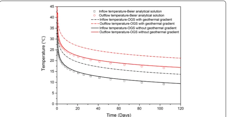
The numerical result was compared against analytical solution in order to verify its cor-rectness. Simulated soil temperature distribution indicates that the DBHE operation can reach around 100 m away after an simulated operation of 30 years. The geometric model ensures that there is no interference caused by the boundary effect. The analytical solu-tion employed for verificasolu-tion here was proposed by Beier et al. (2014). The comparison of numerical and analytical solution is presented in Fig. 2, where the inflow and outflow temperature from the DBHE was compared. It can be found that two results fit very well over the period of one heating season. The largest relative error is only around 2.3%, meaning there is temperature difference of less than 0.7 °C after operation for 103 days. Among the various analytical solutions that can model the DBHE operation (Li and Lai 2015), Beier’s solution was applied in this work to compare with numerical results because it is a transient heat transfer model that explicitly simulates the temperatures on inner and annulus pipes, instead of only calculating the mean temperature approxi-mation in the borehole. In the analytical and numerical models, the calculated thermal resistances between the pipe and the soil parts have minor differences, leading to the deviation observable in the inflow and outflow temperature profile.
As shown in Fig. 2, such temperature differences will barely have any significant
influence on the system performance, both in short- or long-term analysis. It has to be
mentioned here that the initial geothermal temperature was considered to be homoge-neous, so that the analytical solution can be calculated. This deviation from the reality will lead to a lower evaluation on the DBHE’s performance. With the geothermal gradi-ent applied on the initial condition, the outflow temperature will increase by 4.29 °C after 120 days as predicted by the numerical model, which is much higher than the devia-tion mendevia-tioned above. As Fig. 2 demonstrates the temperature variation of inflow and outflow pipe over time, Fig. 3 depicts the temperature distribution over depth. Here, the vertical temperature distribution of the circulating fluid in DBHE fits the analytical solution very well. The largest relative error is 2.4%, which occurs after operation for 1 day. The maximum temperature difference between Beier’s solution and OGS numerical results is 0.9 °C. As operational time increases, the deviation will be much smaller. The reason behind this phenomenon is that at the beginning of the simulation, temperature of circulation fluid is largely controlled by the thermal resistance between the pipe and the soil. While the heat extraction continues, thermal conductivity of the surrounding soil gradually becomes the more dominating factor. Therefore, the difference in govern-ing equations is havgovern-ing less impact on the predicted temperature values. Based on the above comparison, the numerical model here is successfully verified and can be applied for the analysis of DBHE system performance.
Simulated scenarios
With the verified numerical model, different scenarios were established and simulated. The overview of these scenarios is listed in Table 2. In Fig. 3, the initial soil temperature was considered to be constant and homogeneous for comparison against analytical solu-tion. This assumption is far from reality as it is well known that the soil temperature will gradually increase with depth. Therefore, the modeling scenario #0 was prepared to reflect the natural geothermal gradient. After that, scenario #1A–D was designed with different values of pipe wall thermal conductivity. First, two types of materials were cho-sen for the outer pipe, one was made of steel and the other of concrete. Depending on
whether an insulation layer was added, four different thermal conductivity values can be derived (#1A–D). Details on these conductivity values are listed in Table 3. Desmedt et al. (2012) and Zhang et al. (2015) declared that the application of thermally enhanced grout will improve the performance of the BHE. For the DBHE system, considering the large quantity of grout required to seal a deep borehole, the additionally initial invest-ment needs to be justified by the long-term gain in performance. Also in reality, some companies may choose to skip sealing DBHE outer pipe, or just doing it partially to cut the cost. Therefore, four different values of grout thermal conductivity were simulated including sealing the outer pipe with concrete (#2C), with thermally enhanced grout (#2D), leaving it unfilled (#2A), or filled partially with water (#2B, see Table 4 for details).
Since the sensible heat stored in soil is the main energy source for DBHE system, sen-sitivity analysis regarding the soil properties is also investigated here. As the geother-mal gradient can vary in different places, the initial soil temperature distribution and heat flux into the domain can be different. Based on the ideal geological conditions, four scenarios were designed (#3A–D) with the geothermal gradient increasing from 0.03 to 0.04 °C m−1 (see details in Table 5) along with increasing thermal extraction rates. Then five scenarios were simulated (#4A–E) with different soil thermal conductivity values listed in Table 6. In order to investigate impact of groundwater flow on the performance of the DBHE system, four scenarios (#5A–D) were designed with a 13-m-thick aquifer positioned at three different depths (#5A–C). And there are another five aquifers with Table 2 List of all simulated scenarios and features
Scenario ID Geothermal gradient (°C m−1)
Pipe wall thermal conductivity (W m−1 K−1)
Grout thermal conductivity (W m−1 K−1)
Soil thermal conductivity (W m−1 K−1)
Operation
period (days) Groundwater flow
0 0.03 Const. 1.3 2.5 120 N
1A–D 0.03 Var. 1.3 2.5 120 N
2A–D 0.03 Const. Var. 2.5 120 N
3A–D Var. Const. 1.3 2.5 120 N
4A–E 0.03 Const. 1.3 Var. 120 N
5A–D 0.03 Const. 1.3 2.5 120 Y
6A–B 0.03 Const. 1.3 2.5 10950 (30
years) N
Table 3 Different outer pipe materials with different inner pipes Scenario ID Inner pipe wall thermal
conductivity (W m−1
K−1)
Outer pipe wall thermal conductivity (W m−1
K−1)
Description
1A 0.5 1.3 Concrete outer pipe without heat insula-tion layer on the inner pipe
1B 0.1 1.3 Concrete outer pipe with heat insulation layer on the inner pipe
1C 0.5 20 Steel outer pipe without heat insulation layer on the inner pipe
the thickness of 12 m each further added in upper part of the soil so that the influence of multi-layer aquifers on the system can also be quantified (#5D). The intention here is to systematically reveal how the DBHE system performance changes if the subsurface condition is favorable. To investigate the long-term performance of the DBHE system, scenarios #6A–B were simulated for a period of 30 years long. Preliminary test simula-tion showed that the fluctuating ground surface temperature has barely any influence on the simulated inflow and outflow temperatures. Therefore, the surface temperature was assumed to be constant in all the modeling scenarios.
Results and discussion
Temperature distribution inside the DBHE
In scenario #0, the simulated result of vertical temperature distribution at different oper-ational times is depicted in Fig. 4. It can be found that the circulating fluid temperature quickly drops after the start of operation. This trend will stabilize itself as the surround-ing soil temperature reaches equilibrium with the circulatsurround-ing fluid. When compared with the result without geothermal gradient in Fig. 3, the slope of the inflow temperature increases only slightly within the first 800 m, and this slope is significantly steeper at the Table 4 Parameter values used in the model to represent different grout materials
Scenario ID Grout thermal conductivity
(W m−1 K−1) Description
2A 0.35 Gap filled with half air and half water
2B 0.68 Gap fully saturated with water
2C 1.3 Filled with concrete
2D 2.1 Thermally enhanced material as grout
Table 5 Variation of geothermal gradient with different specific heat extraction rates Scenario ID Geothermal
gradient (°C m−1) Specific heat extraction rate imposed on the DBHE (W m−1) Description
3A 0.03 100 Standard geothermal gradient
3B 0.04 100 Elevated geothermal gradient
3C 0.04 200 Elevated geothermal gradient
3D 0.04 Var. Elevated geothermal gradient
Table 6 Variation of soil thermal conductivity
Scenario ID Soil thermal conductivity
(W m−1 K−1) Heat load on the DBHE system (kW)
4A 2.0 390
4B 2.25 390
4C 2.5 390
4D 2.75 390
depth greater than 800 m. That reveals that due to the presence of the geothermal gradi-ent, heat extraction is more efficient in the lower part of the DBHE. Since the ground surface temperature is ca. 6 °C and the geothermal gradient is configured to be 0.03 °C m−1, the subsurface temperature reaches 30 °C at the depth of 800 m. At depth greater than 800 m, the surrounding soil starts to be hotter than the circulating fluid, leading to a higher heat flux from the surrounding soil into the DBHE.
As explained above, the sensible heat is mainly extracted from the deeper part of the soil, and the DBHE will lose some heat to the surrounding soil when the fluid is pumped upwards. As the operation proceeds, the temperature of upper soil will be gradually heated up. This means, the equilibrium depth originally located at 800 m depth will also be gradually shifted upwards. This feature is unique in the DBHE and cannot be found in shallow single-U or double-U-type of BHEs. As shown in Fig. 4, the inner outflow fluid temperature keeps decreasing from the bottom to the top. This indicates that the heat loss from inner to outer pipe exists throughout the entire DBHE. This also suggests that, if the inner pipe wall can be better insulated (with a lower thermal conductivity), the amount of heat loss will be constrained and the efficiency of the DBHE can be improved.
Heat flux analysis
Based on the simulated temperature presented in the above section, it can be further analyzed to reflect the heat flux distribution between different components in the bore-hole at any time. Over a heating season (from 1 to 119 day), there is a clear trend that can be found in Fig. 5. The blue line, which represents the heat flux from grout to soil, will intersect with the purple line, that refers to the flux from grout to outer pipe. This inter-action point is located at a depth of 800 m at 1 day, and will be gradually shifted upwards to ca. 200 m after 119 days. Physically, this interaction point indicates the location where the heat flux flow into and out of the grout zone equals to zero. This also means that, for the section above this point, DBHE is losing energy to the surrounding soil, while only the section below this point is contributing to the extraction of geothermal energy.
The same process is also indicated in the change of the red line, representing the heat flux going in the annular pipe. There, the value difference between bottom and top of the DBHE will decrease over time. Considering the upper part of soil is heated due to heat loss from the DBHE, the heat flux going into the annular pipe is positive at 1 day. After the operation of 30 days, the same heat flux turns into negative values at the top of the DBHE, suggesting that the ground surface temperature is higher than the inflow temper-ature and the sensible heat in the subsurface is being extracted, and this process is not restricted just to the bottom part. When looking into the black line, which indicates the heat loss from the inner pipe, it can be found that this loss does not change much over time. The absolute amount of heat loss is zero at the bottom of the DBHE, as there is no temperature difference between the inner and annulus pipe, while it increases itself and reaches the maximum near the ground surface. This implies that when applying insula-tion material to cut this heat loss, the material should be applied throughout the entire depth of the inner pipe, not only the upper part.
It is noticed that the heat flux analysis can also be used to check the balance and accu-racy of the numerical model. At a particular time step, the simulated heat flux between the soil and the grout can be integrated over the entire depth of DBHE. The calculated value was compared to the heat extraction rates imposed on the DBHE at that moment. It was found that these values fit well with each other, bearing only a relative deviation of 0.03%. This is more proof that the numerical model is delivering accurate results throughout the entire simulated heating period.
Influence of different pipe materials
The impact of different pipe materials is mainly investigated by varying the pipe wall thermal conductivity values in the numerical model (as listed in Table 3). From scenario #1A to #1D, the outflow temperature of the DBHE and its evolution trend is predicted by the numerical simulation, and the statistical distribution of heat pump COP was then calculated accordingly following Eq. 10. Such distribution over an entire heating season is summarized in Fig. 6. By comparing the result of scenario #1A and scenario #1B, it can be revealed that the heat pump COP will be improved by approx. 7.2% when applying the material with lower thermal conductivity on the inner pipe. On the contrary, if the outer pipe concrete material (scenario #1B) is substituted by steel (scenario #1D), the average COP value can only be improved by 1.57%. It can be concluded that although both insulating the inner pipe and enhancing the outer pipe thermal conductivity will improve the system performance, the outer pipe wall has a relatively minor impact. In real projects, installing the concrete outer pipe instead of steel will save a lot of initial investment, as the DBHE is typically 2 to 3 km long. Therefore, it is economically more attractive to use low thermally conductive material (such as high-density polyethylene— HDPE) as the inner pipe.
Influence of grout thermal conductivity
(scenario #2A) to 2.1 W m−1 K−1 (scenario #2D) and the average COP of coupled heat pump will increase by 1.05. The average COP (cf. Fig. 7b) will be improved by 9.88% if the thermally enhanced material (scenario #2D) is used as grout instead of concrete (sce-nario #2C) and the outflow temperature will increase by 6.24 °C at the end of the season. This analysis indicates that thermally enhanced grout material can significantly improve the heat transfer between the borehole wall and the outer pipe, thus leading to a higher-system performance. Scenarios #2A and #2B represent the cases where the DBHE is not properly sealed. For #2A, it is assumed that the gap between the DBHE and the sur-rounding soil is filled by half water and half air. Scenario #2B refers to those boreholes fully filled with water. As shown in Fig. 7, in these two scenarios, the outflow tempera-ture in #2B will be 4.15 °C higher, and the corresponding COP will also be improved by 7.3 %. It can be concluded that the system performance will greatly deteriorate if the gap between borehole wall and surrounding soil is not properly sealed.
Influence of geothermal gradient
In the simulated scenarios, the large portion of extracted geothermal energy is coming from the sensible heat stored in the surrounding soil. Therefore, the initial soil tempera-ture distribution can be reflected in the average geothermal gradient. To achieve this, steady-state heat transport simulations were conducted with the amount of heat flux
imposed at the bottom of the model domain that correspond to the 0.03 °C m−1 and
0.04 °C m−1 geothermal gradient. These simulations produced two different linear distri-butions of soil temperature over the entire depth, which shows the equilibrium state of an undisturbed subsurface. These two distributions are then applied in scenarios #3A to #3D as initial condition for the soil temperature.
With the initial soil temperature fixed, scenarios #3A to #3D (cf. Table 5) were simu-lated to investigate the impact of different geothermal gradients. The numerical results are presented and compared in Fig. 8. Fig. 8a shows that the outflow temperature of the DBHE increases by 13.41 °C when the geothermal gradient is elevated from 0.03 to
0.04 °C m−1, with the specific heat extraction rate kept the same at 100 W m−1. This sug-gests that a higher heat extraction rate can be applied to the same system when a higher geothermal gradient is present. Following this thought, the extraction rate was increased to 200 W m−1 (scenario #3C). It can be found that in this case that the inflow tempera-ture is quickly dropping and it will approach 0 °C after only about 50 days. In reality, this means the DBHE is heavily overloaded and heat pump system is very likely to automati-cally shut down.
To find out the maximum sustainable heat load of the DBHE under the geothermal gradient of 0.04 °C m−1, the imposed thermal load was then adjusted as shown in Fig. 8b according to the trend of energy demand during winter. The average specific heat extrac-tion rate in one heating season is 157.3 W m−1. Under this condition, the lowest out-flow temperature is 16.32 °C and the final outout-flow temperature is 30.09 °C at the end of one heating season. As shown in Fig. 8b, the lowest inflow temperature is approaching
2 °C when the instantaneous heat load reaches 500 kW (192.3 W m−1). Combined with numerical results of scenario #3C, it can be concluded that the sustainable specific heat extraction rate can be enlarged bigger than 150 W m−1 but smaller than 200 W m−1.
Influence of soil thermal conductivity
As shown in the previous section, the geothermal gradient regulates the initial soil temperature over depth, thus further determining the amount of sensible heat avail-able for extraction. On the other hand, the amount of extractavail-able heat within a unit time period is also controlled by the soil thermal conductivity. With this assumption in mind, five scenarios were designed with various soil thermal conductivity values to investigate its influence (see Table 6). As shown in Fig. 9, when the soil thermal con-ductivity increases from 2.0 W m−1 K−1 (scenario #4A) to 3.0 W m−1 K−1 (scenario #4E), the outflow temperature of the DBHE will be elevated by 9.45 °C, accounting for
a 15% increase. It is also noticed that the marginal performance gain from increasing soil thermal conductivity is gradually decreasing. For example, when the soil thermal conductivity is increased from 2.0 W m−1 K−1 (scenario #4A) to 2.25 W m−1 K−1 (sce-nario #4B), the outflow temperature will increase by 2.97 °C. When the conductivity is further increased from 2.75 W m−1 K−1 (scenario #4D) to 3.0 W m−1 K−1 (scenario #4E), the elevation is only 1.57 °C. Fig. 9 also reveals that a higher thermal conduc-tivity value will lead to a faster recovery in the outflow temperature. By comparing the soil thermal conductivity of 2.0 W m−1 K−1 (scenario #4A) and 3.0 W m−1 K−1 (scenario #4E), there will be an outflow temperature difference of 0.89 °C at the end of the recovery period. Although it looks insignificant, such difference in outflow tem-perature will be accumulated over decades of operation. This means that with the low soil thermal conductivity, the inflow temperature of the DBHE is likely to approach 0 °C much earlier than in the high conductivity case.
Influence of groundwater flow
It is well known that groundwater flow will greatly enhance the performance of shallow BHEs. For the DBHE system, groundwater containing aquifers are not likely to cover the entire length of the borehole. It is more likely that aquifers with high permeabil-ity are intersecting the DBHE at various depths. To reflect this realpermeabil-ity, a total of four scenarios were designed as listed in Table 7. In scenarios #5A to #5C, an aquifer with
Fig. 9 Influence of soil thermal conductivity on the outflow temperature of DBHE
Table 7 Groundwater flow in the subsurface
Scenario ID Aquifer number Aquifer thickness (m) Aquifer location
5A 1 13 395 m
5B 1 13 1395 m
5C 1 13 2395 m
5D 6 12 * 5 and 13 * 1 Distributed every
13 m thickness was assumed to be located at different depths, and there is a horizon-tal groundwater flow with a Darcy velocity of 0.368 m day−1 in the aquifer. In scenario #5D, five aquifers with the thickness of 12 m were further added, with a 50-m interval between the depth of 50 m down to 360 m, mimicking the very porous and fully satu-rated shallow sediments. The Darcy velocity in these aquifers was assumed to be of the same value, which translates to about 130 m year−1 of horizontal groundwater move-ment. These scenarios were designed to reveal, whether the groundwater in single or multiple aquifers will increase the sustainable heat extraction rate of the DBHE.
The simulated numerical results presented in Fig. 10 indicate that the groundwater movement has only very minor influence on the DBHE performance. The outflow tem-perature at the end of one heating season remains almost the same in all four scenarios regardless of the number or locations of aquifers. In scenario #5D, where a total of six aquifers were added, the outflow temperature at the end of the heating season is only 0.1 °C less than that the baseline case where no groundwater flow was considered. In this
case, the groundwater flow in shallow aquifers is actually increasing the heat loss of the DBHE.
The temperature peaks in Fig. 10b at a depth of 2395 m is a clear indication of deep aquifers’ influence (scenario #5C). In comparison to other scenarios, the extracted ther-mal energy via the DBHE is mainly from the bottom part of the soil, as already dem-onstrated by the heat flux analysis. Deep aquifers have higher temperature and provide extra thermal energy through the groundwater advection process. But heat energy sup-plied by deep aquifers only accounts for a tiny ratio of total amount of extracted energy. And such extra energy supplied by deep aquifers will be distributed along the depth of the DBHE during the circulating fluid flowing process so that the outflow temperature of the DBHE will not be changed much. All in all, since the overall depth of the aquifer in the investigated scenarios is still a small portion of the DBHE length, the amount of thermal energy recharged (deep aquifers) or discharged (shallow aquifers) through the groundwater advection takes only a small part in the overall extracted heat from the deep subsurface. This feature is largely due to the extended length of the DBHE, which is different from shallow BHEs.
It should be noted that the average soil thermal conductivity will be affected due to the presence of aquifers in the subsurface. When the porous media is fully saturated or partially saturated with water, the air in pores will be substituted and the average soil thermal conductivity will increase so that the system performance will be improved as discussed before.
Long‑term sustainability analysis
As the DBHE system is constructed for building heating purposes, it has to be running for a long period of time (e.g., 30 years) in order to cover its high initial investment. In the long term, the system is actually constrained by the lowest temperature of the cir-culating fluid that enters and leaves the heat pump. Based on communication with the equipment vendors, it is learned that the minimum outflow temperature of the DBHE has to be kept higher than 4 °C, and the inflow temperature should be above the freez-ing point, so that unfavorable freezfreez-ing and thawfreez-ing processes can be avoided around the DBHE. With such criteria in mind, the numerical models were simulated with a range of different thermal loads on the DBHE, ranging from 50 W m−1 up to 200 W m−1 of spe-cific heat extraction rate. In these long-term simulations, the domain size was carefully checked to guarantee that there are no interactions between the thermal plume and the lateral boundaries of the domain.
be kept at around 17.2 °C. It is thus safe to conclude that a specific heat exchange rate of 100 W m−1 can be sustainably achieved on such a DBHE system for even longer period of time. When the thermal load increases to 125 W m−1, the minimum inflow tempera-ture will be approaching 0 °C (cf. Fig. 11b) after about 20 years of operation. When this happens, the heat pump must be already operating at a very low efficiency and will not be economical. But it is noticeable that the outflow temperature can still reach 9.93 °C; in other words, there is still space to operate as long as the thermal load on the DBHE was kept the same.
Efficiency analysis
In the DBHE system, due to the presence of deep boreholes and long pipelines, the hydraulic loss is considerably higher than the shallow BHE system. Therefore, when ana-lyzing the system efficiency, it is vital to include the electricity consumption by the cir-culating pump. With this fact in mind, the coefficient of system performance is defined
in Eq. 11, which is the ratio of total electricity consumption over the amount of ther-mal energy supplied to the building. Assuming the outflow temperature of the DBHE is 20 °C with the baseline parameters presented in Table 1, the COP of heat pump equals to 5.585 according to Eq. 10, i.e., the electricity consumed by the heat pump accounts for 56706.65 W. Meanwhile, there will be a electricity consumption of 6943 W required by the circulating pump, which is calculated by Eq. 12 considering the hydraulic loss in annulus and inner pipe. By comparing the two types of electricity consumption, it can be seen that the circulating pump will actually consume 12.24% of the total electricity needed by the entire system. When the above information is plugged into Eq. 11, it can be found that the calculated CSP value will be 0.61 less than the COP. Over the entire life span of the DBHE system, the electricity consumed by the circulating pump is almost constant, while the heat pump consumption will be varied depending on the DBHE flow temperature and the thermal load from the building. In general, as the DBHE out-flow temperature is gradually dropping, the heat pump consumption will increase, and the percentage of circulating pump will decrease.
As mentioned above, the system will shut down in reality when the outflow tempera-ture of the DBHE is below 4 °C, meanwhile the temperatempera-ture difference cannot be bigger than 4 °C if the outflow temperature is approaching 4 °C. In other words, according to the parameters presented in this work, when the CSP is lower than 3.7 and COP of the heat pump is lower than 4.3, then the system is very likely to shut down automatically.
Taking advantage of the simulated inflow and outflow temperature, the temperature recovery ratio of every year was also calculated and its evolution is plotted in Fig. 12
for analysis, along with the statistical distribution of CSP values over 30 years of opera-tion. It can be found that the temperature recovery ratio is lower than 99.5% in the first 5 years, and gradually increases afterwards. After 30 years, this ratio stabilizes at 99.91% and 99.89% for the 100 W m−1 and 125 W m−1, respectively. The variation range of recovery ratio is within 0.03% in the last ten recovery seasons and it approaches 100% in both long-term scenarios, indicating that the heat energy extracted during heating sea-son is nearly fully recovered. It can be also calculated that over 30 years’ operation, the
average CSP with 100 W m−1 specific heat extraction rate will be 0.24 higher than that in the 125 W m−1 case.
Conclusions
Novelty
As stated in the introduction part, the motivation of this work was to investigate factors that influence the performance and sustainability of the DBHE system. The target was achieved by constructing numerical models with the OpenGeoSys software and simulating it with parameters obtained from a pilot project in China. The numerical result was firstly veri-fied against analytical solution and further analyzed to quantify the heat flux variation over depth. Following this methodology, key parameters of interest were varied in the model in order to reveal their impact on the short-term performance, as well as the long-term sus-tainability. The combined impact was integrated into a CSP value, which was proposed as an index to measure the efficiency of the DBHE system.
Main findings
Among all the parameters, the soil thermal conductivity is the most important parameter determining the system performance, as the sensible heat stored in soil is the main energy source. The modeling result also found that the performance of the DBHE system can be improved by substituting the inner pipe with thermally insulated material. For the outer pipe, its thermal conductivity has only limited effect, while the application of thermally enhanced grout material will considerably improve the performance of the system. In loca-tions where the averaged geothermal gradient is 0.04 °C m−1, the sustainable specific heat extraction rate is calculated to be more than 150 W m−1 but smaller than 200 W m−1.
In the long-term scenarios, the sustainability of the system is constrained by the lowest outflow temperature of the DBHE. The outflow temperature should be controlled higher than 4 °C, which provides acceptable efficiency of the heat pump. At the same time, the lowest inflow temperature of the DBHE cannot be 0 °C, which is restricted by the circulat-ing fluid and heat pump capacity. Durcirculat-ing the first 20 years of operation, the lowest outflow temperature of the DBHE quickly decreases in the first 7 to 8 years, and then gradually sta-bilizes after 10 years.
In modeling scenarios where the groundwater flow was considered, the outflow tempera-ture of the DBHE barely changed. In other words, the performance and sustainability of the DBHE system are not affected by the groundwater flow, as the aquifers have only a small percentage penetrated by the DBHE. By calculation of the CSP value, the efficiency of the DBHE system can be quantified. A conclusion can be drawn that the lower threshold of the system efficiency is at a CSP value of 3.7, which corresponds to a heat pump COP of 4.3. When the system is operating below this threshold, it is very likely to be shut down due to low-temperature protection mechanism. However, it should be noticed that the CSP value strongly depends on the pipe structure and flow rate of circulating fluid.
Implications and outlook
building surface area of 11,143 m2, it can only satisfy the heat demand of around 111 apart-ments with heating demand of 35 W m−12. Therefore, in a typical neighborhood located in densely populated urban areas, the heat pump needs to be coupled with several DBHEs. It is a challenge to simulate the complex interaction of such systems with several DBHEs and the connecting pipe network. This will be a topic for future investigation.
List of symbols
Roman letters ˙
Q : thermal power ( M L2T−3 ); c: specific heat capacity ( L2T−2−1 ); D: diameter (L); H: thermal sink/source term ( M L−1T−3 ); L: borehole length (L); P: pressure ( M L−1T−2 ); Q: flow rate ( L3T−1 ); q
n : normal heat flux ( M T−3 ); r: radius (L); Re: Reynolds num-ber (1); T: temperature ( ); t: pipe wall thickness (L); v: velocity ( L T−1 ); W: electricity ( M L2T−3).
Greek letters
β : thermal expansion coefficient ( −1 ); ǫ : soil porosity (1); η : efficiency of the circulating pump (1); Ŵ : boundary; : tensor of thermal hydrodynamic dispersion ( M L T−3−1 );
: thermal conductivity ( M L T−3−1 ); µ : viscosity ( M L−1T−1 ); : domain; : heat exchange coefficient ( M T−3−1 ); ρ : density ( M L−3).
Subscripts
b: borehole; cp: circulating pump; f: fluid in the soil; ff: between inflow and outflow; fig: between inflow and grout; g: grout; gs: between grout and soil; h: hydraulic; hp: heat pump; i: inner pipe; o: outer pipe; r: circulating fluid (refrigerant); s: soil
Acknowledgements
Funding for the project was provided by the German Federal Ministry of Economic Affairs and Energy (BMWi) under Grant No. 03ET6122B (“ANGUS II: Impacts of the use of the geological subsurface for thermal, electrical or material energy storage in the context of transition to renewable energy sources—Integration of subsurface storage technologies into the energy system transformation using the example of Schleswig-Holstein as a model area”) and is gratefully acknowl-edged. The research was supported as part of the GEMex project funded by the European Union’s Horizon 2020 pro-gramme for Research and Innovation under Grant agreement No. 727550. Also, the first author (Chaofan Chen) would like to acknowledge the financial support from the China Scholarship Council (CSC) for his Ph.D. study in Germany. Authors’ contributions
This study is part of the Ph.D work of CC supervised by HS and OK. DN constructed the data structure for the DBHE feature in the OGS software. YK provided fundamental parameters of the DBHE system from northern China. KT offered suggestions regarding COP of heat pump and references of calculating CSP value. All authors read and approved the final manuscript.
Availability of data and materials
The DBHE modeling feature presented in this work has been included in the OpenGeoSys (OGS) software since version 6.2. Interested readers may obtain source code and corresponding benchmarks from the OGS website https ://www. openg eosys .org/.
Competing interests
The authors declare that they have no competing interests.
Author details
1 Helmholtz Centre for Environmental Research (UFZ), Permoserstr. 15, 04318 Leipzig, Germany. 2 Applied Environmental
Systems Analysis, Dresden University of Technology, 01069 Dresden, Germany. 3 Freiberg University of Mining and
Tech-nology, 09599 Freiberg, Germany. 4 Institute of Geology and Geophysics, Chinese Academy of Sciences, Beijing 100029,
China. 5 China University of Mining and Technology (Beijing), Beijing 100083, China. 6 Department of Environmental
Sciences, University of California, Riverside, CA 92521, USA.
References
Acuña J, Palm B. Distributed thermal response tests on pipe-in-pipe borehole heat exchangers. Appl Energy. 2013;109:312–20.
Al-Khoury R, Kölbel T, Schramedei R. Efficient numerical modeling of borehole heat exchangers. Comput Geosci. 2010;36(10):1301–15.
Beier RA, Holloway WA. Changes in the thermal performance of horizontal boreholes with time. Appl Therm Eng. 2015;78:1–8. Beier RA, Acuña J, Mogensen P, Palm B. Transient heat transfer in a coaxial borehole heat exchanger. Geothermics.
2014;51:470–82.
Bu X, Ma W, Li H. Geothermal energy production utilizing abandoned oil and gas wells. Renew Energy. 2012;41:80–5. Cai W, Wang F, Liu J, Wang Z, Ma Z. Experimental and numerical investigation of heat transfer performance and sustainability
of deep borehole heat exchangers coupled with ground source heat pump systems. Appl Therm Eng. 2018;149:975–86. Casasso A, Sethi R. Efficiency of closed loop geothermal heat pumps: a sensitivity analysis. Renew Energy. 2014;62:737–46. Cui Y, Zhu J, Twaha S, Riffat S. A comprehensive review on 2D and 3D models of vertical ground heat exchangers. Renew
Sustain Energy Rev. 2018;94:84–114.
Desmedt J, Van Bael J, Hoes H, Robeyn N. Experimental performance of borehole heat exchangers and grouting materials for ground source heat pumps. Int J Energy Res. 2012;36(13):1238–46.
FEFLOW: finite element modeling of flow, mass and heat transport in porous and fractured media. Berlin: Springer Science & Business Media; 2013.
Diersch HJ, Bauer D, Heidemann W, Rühaak W, Schätzl P. Finite element modeling of borehole heat exchanger systems: part 1. Fundamentals. Comput Geosci. 2011a;37(8):1122–35.
Diersch HJ, Bauer D, Heidemann W, Rühaak W, Schätzl P. Finite element modeling of borehole heat exchanger systems: part 2. Numerical simulation. Comput Geosci. 2011b;37(8):1136–47.
Dijkshoorn L, Speer S, Pechnig R. Measurements and design calculations for a deep coaxial borehole heat exchanger in Aachen, Germany. Int J Geophys. 2013. https ://doi.org/10.1155/2013/91654 1.
Falcone G, Liu X, Okech RR, Seyidov F, Teodoriu C. Assessment of deep geothermal energy exploitation methods: the need for novel single-well solutions. Energy. 2018;160:54–63.
Fang L, Diao N, Shao Z, Zhu K, Fang Z. A computationally efficient numerical model for heat transfer simulation of deep borehole heat exchangers. Energy Build. 2018;167:79–88.
Galgaro A, Farina Z, Emmi G, De Carli M. Feasibility analysis of a borehole heat exchanger (BHE) array to be installed in high geothermal flux area: the case of the Euganean Thermal Basin, Italy. Renew Energy. 2015;78:93–104.
Gordon D, Bolisetti T, Ting DS, Reitsma S. A physical and semi-analytical comparison between coaxial bhe designs considering various piping materials. Energy. 2017;141:1610–21.
Hein P, Kolditz O, Görke UJ, Bucher A, Shao H. A numerical study on the sustainability and efficiency of borehole heat exchanger coupled ground source heat pump systems. Appl Therm Eng. 2016a;100:421–33.
Hein P, Zhu K, Bucher A, Kolditz O, Pang Z, Shao H. Quantification of exploitable shallow geothermal energy by using bore-hole heat exchanger coupled ground source heat pump systems. Energy Convers Manag. 2016b;127:80–9. Holmberg H, Acuña J, Næss E, Sønju OK. Thermal evaluation of coaxial deep borehole heat exchangers. Renew Energy.
2016;97:65–76.
Kahraman A, Çelebi A. Investigation of the performance of a heat pump using waste water as a heat source. Energies. 2009;2(3):697–713.
Kohl T, Brenni R, Eugster W. System performance of a deep borehole heat exchanger. Geothermics. 2002;31(6):687–708. Kolditz O, Bauer S, Bilke L, Böttcher N, Delfs JO, Fischer T, Görke UJ, Kalbacher T, Kosakowski G, McDermott C. Opengeosys: an
open-source initiative for numerical simulation of thermo-hydro-mechanical/chemical (THM/C) processes in porous media. Environ Earth Sci. 2012;67(2):589–99.
Kong YL, Chen CF, Shao HB, Pang ZH, Xiong LP, Wang JY. Principle and capacity quantification of deep-borehole heat exchangers. Chin J Geophys. 2017;60(12):4741–52.
Lazzari S, Priarone A, Zanchini E. Long-term performance of bhe (borehole heat exchanger) fields with negligible groundwa-ter movement. Energy. 2010;35(12):4966–74.
Le Lous M, Larroque F, Dupuy A, Moignard A. Thermal performance of a deep borehole heat exchanger: insights from a synthetic coupled heat and flow model. Geothermics. 2015;57:157–72.
Lhendup T, Aye L, Fuller RJ. In-situ measurement of borehole thermal properties in melbourne. Appl Therm Eng. 2014;73(1):287–95.
Li M, Lai AC. Review of analytical models for heat transfer by vertical ground heat exchangers (GHEs): a perspective of time and space scales. Appl Energy. 2015;151:178–91.
Ni L, Dong J, Yao Y, Shen C, Qv D, Zhang X. A review of heat pump systems for heating and cooling of buildings in china in the last decade. Renew Energy. 2015;84:30–45.
Rivera JA, Blum P, Bayer P. A finite line source model with cauchy-type top boundary conditions for simulating near surface effects on borehole heat exchangers. Energy. 2016;98:50–63.
Shao H, Hein P, Sachse A, Kolditz O. Geoenergy modeling II: shallow geothermal systems. Berlin: Springer; 2016. Shi Y, Song X, Li G, Yang R, Shen Z, Lyu Z. Numerical investigation on the reservoir heat production capacity of a downhole
heat exchanger geothermal system. Geothermics. 2018;72:163–9.
Soldo V, Borović S, Lepoša L, Boban L. Comparison of different methods for ground thermal properties determination in a clastic sedimentary environment. Geothermics. 2016;61:1–11.
Tang F, Nowamooz H. Long-term performance of a shallow borehole heat exchanger installed in a geothermal field of alsace region. Renew Energy. 2018;128:210–22.
Wagner V, Bayer P, Bisch G, Kübert M, Blum P. Hydraulic characterization of aquifers by thermal response testing: validation by large-scale tank and field experiments. Water Resour Res. 2014;50(1):71–85.
Welsch B, Rühaak W, Schulte DO, Bär K, Sass I. Characteristics of medium deep borehole thermal energy storage. Int J Energy Res. 2016;40(13):1855–68.
Wu Q, Tu K, Sun H, Chen C. Investigation on the sustainability and efficiency of single-well circulation (SWC) groundwater heat pump systems. Renew Energy. 2019;130:656–66.
Zhang W, Yang H, Lu L, Fang Z. Investigation on influential factors of engineering design of geothermal heat exchangers. Appl Therm Eng. 2015;84:310–9.
Zheng T, Shao H, Schelenz S, Hein P, Vienken T, Pang Z, Kolditz O, Nagel T. Efficiency and economic analysis of utilizing latent heat from groundwater freezing in the context of borehole heat exchanger coupled ground source heat pump sys-tems. Appl Therm Eng. 2016;105:314–26.
Publisher’s Note