On modeling and complete solutions to general fixpoint problems in multi-scale systems with applications

R E S E A R C H

Open Access

On modeling and complete solutions to

general fixpoint problems in multi-scale

systems with applications

Ning Ruan

_{and David Yang Gao}

*_{Correspondence:} [email protected] 1_{School of Science and Information} Technology, Federation University Australia, Ballarat, Australia

Abstract

This paper revisits the well-studied fixed point problem from a unified viewpoint of mathematical modeling and canonical duality theory, i.e., the general fixed point problem is first reformulated as a nonconvex optimization problem, its

well-posedness is discussed based on the objectivity principle in continuum physics; then the canonical duality theory is applied for solving this challenging problem to obtain not only all fixed points, but also their stability properties. Applications are illustrated by problems governed by nonconvex polynomial, exponential, and logarithmic operators. This paper shows that within the framework of the canonical duality theory, there is no difference between the fixed point problems and nonconvex analysis/optimization in multidisciplinary studies.

MSC: 47H10; 47H14; 55M05; 65K10

Keywords: Fixed point; Properly-posed problem; Nonconvex optimization; Canonical duality theory; Mathematical modeling; Multidisciplinary studies

1 Introduction

The fixed point problem is a well-established subject in the area of nonlinear analysis [3,

4,7], which is usually formulated in the following form:

(P0) : x=F(x), (1)

whereF :Xa →Xa is a nonlinear mapping andXa is a subset of a normed space X.

Problem (P0) appears extensively in engineering and sciences, for example, in equilibrium problems, mathematical economics, game theory, and numerical methods for nonlinear dynamical systems. A general form of the equilibrium problem was first considered by Nikaido and Isoda in 1955 as an auxiliary problem to establish existence results for Nash equilibrium points in non-cooperative games [43–46]. Mathematically speaking, the non-linear operatorF(x) could be any arbitrarily given vector-valued function. Therefore, the formula (P0) for the fixed point problem is too abstract. Although it can be used to “model” a large class of mathematical problems, one must pay a price: it is impossible to develop a unified mathematical theory with powerful real-world applications. This dilemma is due to a gap between mathematics and physics. As indicated by V.I. Arnold [1]:“In the middle

of the twentieth century it was attempted to divide physics and mathematics. The con-sequences turned out to be catastrophic.” Indeed, during the past sixty years extensive research on the fixed point problems has been mainly focused on this abstract form. It turns out that the majority theories and methods for solving this nonlinear problem are based on linear iteration [33,34,47,50]. This paper will provide a different approach. For simplicity’s sake, we assume thatXais a convex open set inRnwith a normxinduced

by the bilinear form∗,∗:X×X→R.

Lemma 1 If F is a potential operator,i.e.,there exists a real-valued function P:Xa→R

such that F(x) =∇P(x),then(P0)is equivalent to the following stationary point problem:

¯

x=argsta

(x) =P(x) –1 2x

2_∀x∈X a

. (2)

Otherwise, (P0)is equivalent to the following global minimization problem:

¯

x=arg min

(x) =1

2F(x) – x

2_∀ x∈Xa

. (3)

Proof First we assume thatF(x) is a potential operator, then x is a stationary point of(x) if and only if∇(x) =∇P(x) – x = 0, thus, x is also a solution to (P0) sinceF(x) =∇P(x).

Now we assume thatF(x) is not a potential operator. By the fact that(x) =1₂F(x) –

x2≥0∀x∈X, the vectorx¯is a global minimizer of(x) if and only ifF(x¯) –x¯= 0. Thus,

¯

xmust be a solution to (P0).

By the facts that the global minimizer of an unconstrained optimization problem must be a stationary point and

1

2F(x) – x

2

=P(x) –1 2x

2_{, P(x) =}1

2

F(x),F(x)–x,F(x)+x2, (4) the global minimization problem (3) is a special case of the stationary point problem (2). Mathematically speaking, if a fixed point problem has a trivial solution, thenF(x) must be a homogeneous operator, i.e.,F(0) = 0. For general problems,F(x) should have a nonho-mogeneous term f∈Rn_{. Thus, we can let}

P(x) =W(Dx) –x, f, (5)

whereD:X→W⊂Rm_{is a linear operator,W:W→Ris a so-calledobjective function.}

Objectivity is a basic concept in continuum physics [6,41] and mathematical modeling [18,19]. Its mathematical definition is given in Gao’s book (Definition 6.1.2 [11]).

Definition 1(Objectivity) LetRbe a proper orthogonal group, i.e., R∈Rif and only if

RT= R–1_{,detR= 1. A setW}

ais said to be objective if

Rw∈Wa ∀w∈Wa,∀R∈R.

A real-valued functionW:Wa→Ris said to be objective if

Geometrically speaking, an objective function does not depend on rigid rotation of the system considered, but only on certain measure of its variable. In the Euclidean space

W⊂Rm_{, the simplest objective function is the2-normwinR}m _{as we haveRw}2₌ wTRTRw=w2∀R∈R. For generalF(x), we can see from (4) that1

2F(x) T_and1

2x 2

are objective functions. By the fact that x =F(x), we know thatx,F(x)is also an objective function. Therefore, for a given fixed point problem, the corresponding(x) is naturally an objective function.

Physically, an objective function is governed by the intrinsic physical law of the system, which does not depend on observers. Because of Noether’s theorem, the objective func-tionW(w) should be a SO(n)-invariant and this invariant is equivalent to a certain con-servation law (see Sect. 6.1.2 [11]). Therefore, objectivity is essential for any real-world mathematical models. It was emphasized by P.G. Ciarlet that the objectivity is not an as-sumption, but an axiom [6].

From the viewpoint of systems theory, if x represents the output (or the state, config-uration, etc.) of the system, then the nonhomogeneous term f can be viewed as the in-put (or the control, applied force, etc.), which depends on each given problem. Corre-spondingly, the linear termx, fin (5) can be called thesubjective function[18,19]. Let

Xa={x∈X|Dx∈Wa}. The fixed point problem (P0) can be reformulated into the

fol-lowing stationary point problem:

(P) :x¯=argsta

(x) =W(Dx) –1 2x

2_{–x, f∀x∈X} a

. (7)

From the theory of nonconvex analysis, any nonconvex function can be written as a d.c. (deference of convex) function [35]. Therefore, the fixed point problem is actually equivalent to a d.c. programming problem. By the fact thatX andW are two different spaces with different scales (dimensions), the problem (P) can be used to study general problems in multi-scale complex systems.

For a potential operator, a fixed point is just a stationary point, which can be easily found by traditional linear iteration methods. For a non-potential operator, the fixed point must be a global minimizer. Due to the lack of global optimality condition in the traditional theory of nonlinear optimization, to solve a general nonconvex minimization problem is considered to be NP-hard in global optimization and computer science. However, this paper will show that many of these nonconvex problems can be solved in an elegant way.

2 Methods

According to the Brouwer fixed point theorem, we know that any continuous function from the closed unit ball in an n-dimensional Euclidean space to itself must have a fixed point. Generally speaking, for any given nontrivial input, a well-defined system should have at least one nontrivial response.

Definition 2(Properly- and well-posed problems [18]) The problem (P) is called prop-erly posed if, for any given nontrivial input f= 0, it has at least one nontrivial solution. It is called well-posed if the solution is unique.

speaking, any real-world problems should be well-posed since all natural phenomena exist uniquely. But practically, it is difficult to model a real-world problem precisely. Therefore, properly posed problems are allowed for the canonical duality theory. This definition is important for understanding challenging problems in complex systems.

Example1 (Manufacturing/production systems) In management science, the output is a vector x∈Rn_{, which could represent the products of a manufacture company. The input} f∈Rn_{can be considered as market price (or demand). Therefore, the subjective function} x, f= xT_{fin this example is the total income of the company. The products are produced}

by workers w∈Rm_{. Due to the cooperation, we have w =DxandD∈R}m×n_{is a matrix.}

Workers are paid salaryσ=∂W(w), therefore, the objective functionW(w) is the cost (in this example,W is not necessarily objective since the company is a man-made system). Let 1₂αx2_{be the profit that the company must make, whereα> 0 is a parameter, then} (x) =W(Dx) +1₂αx2_{– x}T_{fis thetargetand the minimization problemmin(x) leads}

to the equilibrium equation

αx= f –DT∂wW(Dx).

This is a fixed point problem. The cost functionW(w) could be convex for a small com-pany, but usually nonconvex for big companies to allow some people have the same salaries.

Example 2 (Lagrange mechanics) In analytical mechanics, the configuration x∈X ⊂

C1_[I;Rn_{] is a continuous vector-valued function of timet∈I⊂R. Its components{xi}}

(i= 1, . . . ,n) are known as theLagrangian coordinates. The input f(t) is a given force vec-tor function inRn_{. Therefore, the subjective functional in this case isx, f=}

Ix(t)·f(t) dt.

The total action of the system is

I

L(x,x˙) dt, L=T(x˙) –V(x),

whereTis the kinetic energy density,Vis the potential density, andL=T–Vis the stan-dardLagrangian density. In this case, the linear operatorD=∂t is a derivative with time.

Together,(x) =_I[T(x˙) –V(x) – xT_{f] dtis called thetotal action. For Newton}

mechan-ics, the kinetic energy is a quadratic (objective) functionT(v) =1₂mv2_{. Its stationary}

condition leads to theEuler–Lagrange equation:

–mx¨= f +∇V(x). (8)

Finite difference method for solving this second-order differential equation leads to a fixed point problem [42]. It is well known that if the potential energyV(x) is convex, the operator

F= f +∇V(x) is monotone and the problem (P0) has a stable fixed point solution. Corre-spondingly, the system has a stable trajectory. Otherwise, the system could have chaotic solutions. The relation between chaos in nonlinear dynamical systems and NP-hardness in computer science has been discovered recently [37].

was proposed by Gao in 1996 [8], which is governed by a forth-order nonlinear differential equation:

χxxxx–

3 2αχ

2

xχxx+λχxx=q, (9)

whereχ(x) is the deflection of the beam, which is a scaler-valued function over its domain [0,L], whereLis the beam length,α> 0 is a material constant, the parameterλdepends on the axial force, andq(x) is a given distributed lateral load. Clearly, this nonlinear deferential equation can be written in the following fixed point problem:

χ(x) =Fx,χ(x), F(x,χ) =

x 0 t 0 s 0 α 1 2χ 3 x –λχx

dsdtdx+f(x), (10)

where the functionf(x) depends on both the lateral loadq(x) and boundary conditions. In this case,F(x,χ(x)) is a nonlinear integration operator. This fixed point problem is equiv-alent to the stationary point problem

χ=argsta

(χ) =

L 0 1 2χ 2 xx+ 1 2α 1 2χ 2 x –λ

2

–q(x)

dxχ∈Xa

. (11)

It was indicated in [13] that ifλ<λc, the Euler buckling load defined by

λc=inf

L 0 χxx2 dx α₀Lχ2

xdx

,

the total potential(χ) is a convex functional, and problem (11) has only one fixed point. In this case, the beam is in a pre-buckling state. It was proved recently (see Lemma 2.1. and Theorem 2.1. in [40]) there exists a constantλG

c >λc such that ifλ>λGc, then(χ)

is nonconvex, i.e., the so-called double-well potential, and the beam is in a post-buckling state. In this case, problem (11) has three fixed pointsχi(x),i= 1, 2, 3, at eachx∈[0,L]:

one global minimizer of(χ), which corresponds to a globally stable post-buckling state of the beam, one local minimizer, which corresponds to a locally stable post-buckling state, and one local maximizer of(χ), which corresponds to an un-buckled state. The com-bination of these three solutions at eachx∈[0,L] forms a solution set with 3∞number of strong solutions on [0,L] to the nonlinear differential equation (9). It was proved in [25] that for certain lateral load distributionsq(x), both the global and local minimum solutions could be nonsmooth and cannot be captured by any Newton-type method. Nu-merical approaches to this nonlinear differential equation are considered to be NP-hard by traditional theories and methods. In order to solve this challenging nonconvex station-ary problem, a canonical dual finite element method has been developed recently [2]. The numerical results shown that the locally stable post-buckling configuration is extremely sensitive to the external loadq(x) and numerical precision used in the program.

For unilateral post-buckling problems, the feasible set Xa has usual inequality

con-straints. For example, a simply supported beam on a rigid foundation subjected to a down-ward lateral loadq(x)∀x∈[0,L], this feasible set is a convex cone:

Xa=

χ(x)∈C2[0,L]|χ(x)≥0∀x∈[0,L],χ(0) =χ(L) = 0,χxx(0) =χxx(L) = 0

Due to the inequality constraint inXa, the stationary condition of problem (11) leads not

only to the so-called variational inequality [38]

L

0

(χ–χ¯)δ(χ¯) dx≥0 ∀χ(x)∈Xa, (12)

whereδ(χ) =χxxxx–3₂αχx2χxx+λχxx–qis the Gâteaux derivative of(χ), but also to

the well-known complementarity condition

χxxxx–

3 2αχ

2

xχxx+λχxx–q

χ(x) = 0 ∀x∈[0,L]. (13)

Since the contact region (i.e., on whichχ(x) = 0) remains unknown till the problem is solved, problem (11) is the combination of the nonlinear free-boundary value problem, non-monotone variational inequality, and the nonconvex variational analysis. This prob-lem could be one of the most challenging probprob-lems in nonconvex analysis, which deserves serious study in the future.

Canonical duality-triality is a methodological theory which can be used not only for modeling complex systems within a unified framework, but also for solving real-world problems with a unified methodology. This theory was developed originally from Gao and Strang’s work for solving the following nonsmooth/nonconvex variational problem [30]:

infP(u) =W(Du) –U(u)|u∈Ua

, (14)

where the variational argument u(x) is a deformation field,Dis a differential operator such that the deformation gradient w =Duis a two-point tensor filed,W(w) is an internal (or free) energy which must be an objective function of w [6,41], whileU(u) is an external energy which must be a linear functional, i.e.,U(u) =u, fsuch that∂U(u) = f is a given external force field. Thus, the differenceP(u) is the well-known total potential energy in nonlinear elasticity. This variational problem (14) covers the most challenging problems in nonconvex analysis and nonlinear partial differential equations. By the objectivity of the free energyW(w), there must exist an objective tensor c = wT_{wand a real-valued function}

V(c) such thatW(w) =V(c(w)) [6]. In finite deformation theory and differential geometry, this objective measure c = cT_{is the well-known Cauchy–Riemann strain tensor andV(c)}

is usually a canonical function, i.e., the duality relation c∗=∂V(c) is a bijection (say the St. Venant–Kirchhoff material [23]). These basic truths in nonlinear analysis lay a foundation for the canonical duality theory. This is the reason why this theory can be used to solve analytically a large class of nonconvex variational problems and their associated partial differential equations, including Einstein’s special relativity equation [12], Kantorovich’s optimal mass transfer problem [39], chaotic dynamics [37,42], global optimization [16,

the discretizedW(w) may not be an objective function, the canonical duality theory has been generalized for solving general nonconvex and discrete optimization problems [5,

15,17,26,27,29,36,49] as well as the most challenging bi-level knapsack problems and topology optimization in multi-scale complex systems [21,22].

However, the well-defined objectivity in nonlinear analysis and physics has been seri-ously misused in optimization and mathematical programming, where the so-called ob-jective function is allowed to be any arbitrarily given function. As a consequence, Gao– Strang’s work has been mistakenly challenged by M.D. Voisei and C. Zalinescu [48]. By oppositely choosing linear functions as the objective functionW(see Example 3.1 in [48]) and nonlinear functions as the external energyU(u) (see Examples 3.2, 3.4, 3.5, and 3.6 in [48]), they produced a series of “counter examples” that led to absurd conclusions includ-ing “The hope for readinclud-ing an optimization theory with diverse applications is ruined by the manner in which [30] is written and the fact that the majority of the results in [30] are false.” These conceptual mistakes verified Arnold’s declaration [1]: “A teacher of mathe-matics, who has not got to grips with at least some of the volumes of the course by Landau and Lifshitz, will then become a relict like the one nowadays who does not know the differ-ence between an open and a closed set.” A comprehensive review on the canonical duality theory and breakthrough from the recent challenges are given in [24].

The goal of this paper is to apply the canonical duality theory for solving the challenging fixed point problem. The rest of this paper is arranged as follows. Based on the concept of objectivity, the canonical dual for the fixed point problem, its analytical solution, and global optimality condition are presented in the next section. Applications to a general fixed point problem with sum of exponential functions and nonconvex polynomial are discussed in Sect.4.1. Analytical solutions for a general fixed point problem with a sum of logarithmic and quadratic functions are given in Sect.4.2. The paper ends with conclu-sions and future work.

3 Results and discussion

According to the canonical duality, the linear measure =Dxcannot be used directly for studying duality relation due to the objectivity. Also, the linear operator cannot change the nonconvexity ofW(Dx). We first introduce the canonical transformation.

Definition 3(Canonical function and canonical transformation) A real-valued function

V:Ea→Ris called canonical if the duality mapping∂V:Ea→Ea∗is one-to-one and onto.

For a given nonconvex functionW:Wa→R, if there exist a geometrically admissible

mapping:Wa→Eaand a canonical functionV:Ea→Rsuch that

W() =V(), (15) then transformation (15) is called the canonical transformation andξ=() is called the canonical measure.

By this definition, the one-to-one duality relationς=∂V(ξ) :Ea→Ea∗implies that the

canonical functionV(ξ) is differentiable and its conjugate functionV∗:E_a∗→Rcan be uniquely defined by the Legendre transformation [11]

whereξ;ςrepresents the bilinear form onEand its dual spaceE∗. In this case,V:Ea→

Ris a canonical function if and only if the following canonical duality relations hold on

Ea×Ea∗:

ς=∂V(ξ) ⇔ ξ=∂V∗(ς) ⇔ V(ξ) +V∗(ς) =ξ;ς. (17)

LetQ(x) =1 2x

2_{+x, f. ReplacingV((x)) in the target function(x) by the Fenchel–}

Young equalityV(ξ) =ξ;ς–V∗(ς), the Gao-Strang total complementary function (see [14]):Xa×Ea∗→Rcan be defined by

(x,ς) =(x);ς–V∗(ς) –Q(x). (18) By this total complementary function, the canonical dual of(x) can be obtained as

d(ς) =inf(x,ς)|x∈X=Q(ς) –V∗(ς), (19) whereQ_:E∗

a →R∪ {–∞}is the so-called-conjugate ofQ(x) defined by (see [14])

Q_{(ς) = sta(x);ς–Q(x)|x∈X. (20)}

Let Sa⊂Ea∗ be an admissible set such that on which Q(ς) is well-defined. If(x) is

a homogeneous quadratic operator, i.e.,(αx) =α2(x), then the total complementary function

(x,ς) = 1 2

x, G(ς)x–V∗(ς) –x, f, (21)

where G(ς) = H(ς) – I, H(ς) =∇x2(x);ς, and I is an identity matrix inX. In this case, the-conjugateQ_{is simply defined by}

Q(ς) = –1 2

G–1(ς)f, f, (22)

andSa={ς∈Ea∗|detG(ς)= 0}. Thus, the canonical dual problem (Pd) can be proposed

in the following:

Pd_{: ς¯ =argsta}d_(ς)|ς∈S a

. (23)

By the canonical duality theory, we have the following results.

Theorem 1(Analytic solution and complementary-dual principle) For a givenf,ifς¯∈S_a

is a solution to(Pd_),then ¯

x= G–1(ς¯)f (24)

is a solution to the problem(P)and

If F(x)is a potential operator,thenx¯ is also a solution to the fixed point problem(P0).If F(x)is a non-potential operator,thenx¯is a solution to the fixed point problem(P0)only if

¯

xis a global minimizer of(x).

Proof By the canonical duality theory we know that (x¯,ς¯) is a critical point of(x,ς) if and only ifx¯is a critical point of(x) andς¯is a critical point ofd(ς). It is easy to prove that the criticality condition∇(x¯,ς¯) = 0 leads to the following canonical equations:

G(ς¯)x¯= f, (x¯) =∂V∗(ς¯). (26)

The first equation is the canonical equilibrium equation, which leads to the analytical so-lution (24). By the canonical duality, the canonical duality equation(x¯) =∂V∗(ς¯) leads to the complementary-duality relation (25). The theorem is proved by Lemma1.

Theorem1shows that the solution to the fixed point problem depends analytically on the canonical dual solution, and there is no duality gap between the primal problem (P) and the canonical dual problem (Pd_{). By the fact that the problem (P) may have many}

fixed points, in order to identify the extremality of these fixed points, we assume that the canonical functionV:Ea→Ris convex and introduce two open sets:

S+ a =

ς∈Sa|G(ς)0

,

S– a =

ς∈Sa|G(ς)≺0

,

where G(ς)0 means that G is a positive definite matrix, and G(ς)≺0 means that G is a negative definite matrix. Also according to the terminology used in the canonical duality theory, a neighborhood of a critical point is an open set containing only one critical point.

Theorem 2(Triality theorem) Suppose thatς¯ is a solution to(Pd_{)andx¯ = G}–1_(ς¯)f.If ¯

ς∈S+

a,thenx¯is a globally stable fixed point and (x¯) =min

x∈Xa

(x) =max

ς∈S+ a

d(ς) =d(ς¯). (27)

Ifς¯∈S_a–,thenx¯is a local maximizer of(x)iffς¯ ∈S_a–is a local maximizer ofdand on the neighborhoodXo×So⊂Xa×Sa–of(x¯,ς¯),we have

(x¯) =max

x∈Xo

(x) =max

ς∈So

d(ς) =d(ς¯). (28)

Moreover,x¯is a locally unstable fixed point of F if it is a potential operator.

Ifς¯ ∈S–

a anddimXa=dimSa,thenx¯is a local minimizer iffς¯∈Sa–is a local minimizer

ofd(ς)and on the neighborhoodXo×So⊂Xa×Sa–,

(x¯) =min

x∈Xo

(x) =min

ς∈So

d(ς) =d(ς¯). (29)

This theorem is an application of the triality theory. Detailed proof can be found in [31]. Statement (27) is the so-calledcanonical min-max duality. This statement shows that the global stable fixed point problem n is equivalent to a concave maximization problem

P

: maxd(ς)|ς∈S_a+. (30)

Since the feasible spaceS+

a is an open convex set, this canonical dual problem can be solved

easily by well-developed nonlinear optimization techniques. The second statement (28) is thecanonical double-max dualityand the third statement (29) is thecanonical double-min duality. For a potential operatorF, these two statements can be used to identify locally unstable and stable fixed points, respectively.

4 Applications

4.1 Exponential and polynomial functions

As our first application, the objective function is assumed to be

W(Dx) =αexp

1 2D1x

2 +1 2β 1 2D2x

2_–λ

2

,

whereD1∈Rm×nandD2∈Rp×nare two given matrices,α,β,λare real numbers. Clearly,

for a givenλ> 0,W(Dx) is nonconvex and

F(x) =∇P(x) =αexp

1 2D1x

2_DT 1D1

x+β

1 2D2x

2_–λDT 2D2

x– f

is a non-monotone operator. In this case, the fixed point problem (P0) can be equivalently written as

¯

x=arg sta x∈Rn

(x) =αexp

1 2D1x

2 +1 2β 1 2D2x

2_–λ

2

–1 2x

2_{– x}T_f

.

Clearly, traditional methods for solving this nonlinear fixed point problem inRnare diffi-cult. However, by the canonical duality theory, this problem can be solved easily inR2_.

The canonical measure in this problem can be given as

ξ=(x) =

ξ1 ξ2 = 1 2D1x2 1 2D2x2

: Rn→Ea=

ξ∈R2|ξ1,ξ2≥0

.

Correspondingly, the canonical function is

V(ξ) =

V1(ξ1)

V2(ξ2)

=

αexp(ξ1) 1

2β(ξ2–λ)2

,

and the canonical dual variable is

ς= ς1 ς2 =

∇V1(ξ1) ∇V2(ξ2)

=

αexp(ξ1)

β(ξ2–λ)

: Ea→Ea∗=

ς∈R2|ς1≥α,ς2≥–λβ

By the Legendre transformation, the conjugate functionV∗(ς) is uniquely defined as

V∗(ς) =

V₁∗(ς1)

V₂∗(ς2)

=

(ln(ς1/α) – 1)ς1 1

2βς 2 2+λς2

.

Since the canonical measure in this application is a homogeneous quadratic operator, the total complementary function:Rn_×E∗

a →Rhas the following form:

(x,ς) = 1 2x

T_{G(ς)x – x}T_f–ln(ς 1/α) – 1

ς1–

1 2βς

2 2+λς2

,

where

G(ς) =ς1DT1D1+ς2DT2D2– I.

On the canonical dual feasible spaceSa={ς= [ς1,ς2]T∈Ea∗|det(G(ς))= 0}, the canonical

dual problem can be formulated as

Pd_{: ς¯ =arg sta}

ς∈Sa

Pd(ς) = –1 2f

T_G–1_{(ς)f –ln(ς1/α) – 1ς1}

–

1 2βς

2 2 +λς2

. (31)

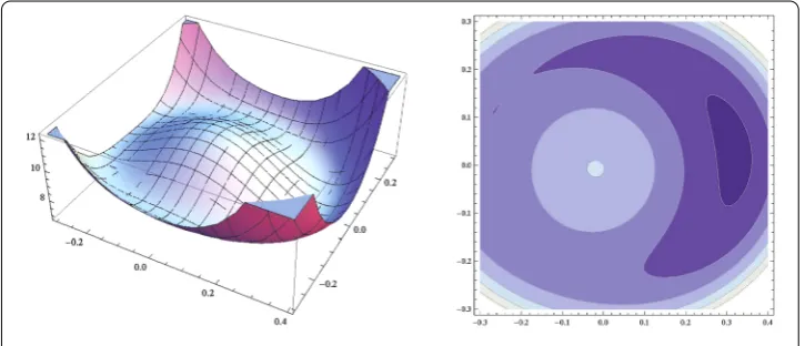
Example1 Letn= 2,α= 6,β= 8,λ= 1, and

D1=

2 0

0 3

, D1=

4 0

0 5

, f=

2 1

,

then the primal function (see Fig.1)

(x1,x2) = 6exp

2x2₁+ 4.5x2₂+ 48x2₁+ 12.5x2₂– 12–1 2

x2₁+x2₂– 2x1–x2.

Figure 2Graphs ofd_{(ς1,ς2) and its contour for Example1}

The corresponding canonical dual function is

d(ς1,ς2)

= –1 2

4

4ς1+ 16ς2– 1+

1 9ς1+ 25ς2– 1

–ς1

ln(ς1/6) – 1

–

1 16ς

2 2+ς2

.

Its graph is shown by Fig.2. It is easy to find that the canonical dual problem (Pd_{) has}

three solutions:

ς1= [7.38697, –1.39206]T∈S_a+,

ς2= [6.00566, –7.97189]T∈S_a–,

ς3= [7.3106, –2.23695]T∈S_a–.

By Theorem1we have three primal solutions:

x1= [0.318731, 0.0325932]T,

x2= [–0.0191337, –0.00683777]T,

x3= [–0.264945, 0.112718]T.

It is easy to check that

x1=dς1= 6.78671,

x2=dς2= 10.0225,

x3=dς3= 7.99906.

By Theorem2we know that x1_{is a global minimizer of(x), x}2_{is a local maximizer of} (x), and x3= [–0.264945, 0.112718]Tis a local minimizer of(x) (see Fig.1). By the fact that

xi₁=F1

xi₂=F2

xi₁,xi₂= 6exp2xi₁+ 4.5xi₂9xi₂+ 88xi₁+ 12.5xi₂– 125xi₂– 1 hold for alli= 1, 2, 3, we know that{xi}(i= 1, 2, 3) are all fixed points. 4.2 Logarithmic and quadratic function

In this application, we let

W(Dx) =c1Dx2+c2Dx2logDx2,

whereD∈Rm×n_{is a matrix,c}

1,c2are real numbers. Clearly,W(Dx) is nonconvex and

F(x) =∇P(x) = 2c1

DTDx+ 2c2

DTDxlogDx2+ 1

is non-monotone. The fixed point problem x =F(x) can be reformulated as

(P) : x¯=argsta

(x) =c1Dx2+c2Dx2logDx2–

1 2x

2_{– x}T_f|x∈Rn

.

By using the canonical measure

ξ=(x) =Dx2: Rn→Ea=R+={ξ∈R|ξ≥0},

the canonical function isV(ξ) =c1ξ+c2ξ(logξ+ 1) and its Legendre conjugate is

V∗(ς) =c2exp

1

c2

(ς–c1) – 1

,

which is convex on its domainE_a∗=R. In this case, we have the total complementary func-tion

(x,ς) = 1 2x

T_{G(ς)x – x}T_f–c 2exp

1

c2

(ς–c1) – 1

,

where G(ς) = 2ςDTD– I and the canonical dual problem is

Pd_{: ς¯=argsta}

Pd(ς) = –1 2f

T_G–1_{(ς)f –c} 2exp

1

c2

(ς–c1) – 1 ς= 0

. (32)

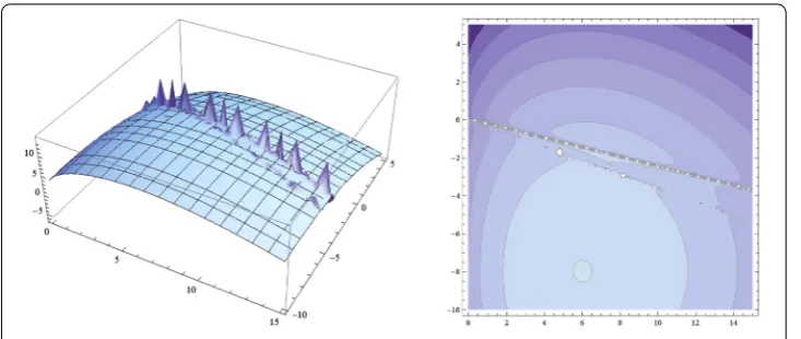
Example2 We first letm=n= 2,c1= –8,c2= 10, and

D=

3 0

0 4

, f=

–5 2

.

The primal function

(x1,x2) = –8

9x2₁+ 16x2₂+ 109x2₁+ 16x2₂log9x2₁+ 16x2₂–1 2

x2₁+x2₂– 5x1+ 2x2

is nonconvex and its graph is shown in Fig.3. The corresponding canonical dual function is

d(ς) = –1 2

25 18ς– 1+

4 32ς– 1

Figure 3Graph of(x1,x2) and its contour for Example2

Figure 4Graph ofd_{(ς) for Example2}

For this example, the one-dimensional canonical dual problem (Pd_{) can be solved easily}

(by using Mathematica) to obtain total three solutions (see Fig.4):

ς1= 0.969642 >ς2= –0.955077 >ς3= –91.0174.

Correspondingly, the three primal solutions are

x1=

–0.303886 0.0666033

, x2=

0.274855 –0.0633664

, x3=

0.00305006 –0.000686446

.

It is easy to check that xi_=F(xi_{),i= 1, 2, 3. Therefore,{x}i_{}are fixed points. Sinceς}1_∈S+ a = {ς∈R|ς> 0}, we know that x1_{is a globally stable fixed point. It is easy to check that x}2

is a locally stable fixed point, x3_{is a locally unstable fixed point, and}

x1=dς1= –9.84726,

x3=dς3= 0.00739894.

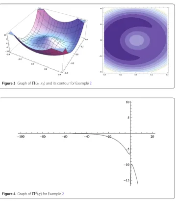
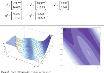
Example3 We now letm= 3,n= 2,c1= –15,c2= 9, and

D=

⎡ ⎢ ⎣

0.3 0.2 0.5 0.6 0.4 0.7

⎤ ⎥

⎦, f=

1 4

,

then the primal function is

(x1,x2) = 9

0.5x2₁+ 1.28x1x2+ 0.89x22

log0.5x2₁+ 1.28x1x2+ 0.89x22

– 150.5x2₁+ 1.28x1x2+ 0.89x22

–1 2

x2₁+x2₂–x1– 4x2.

Its graph is a nonconvex surface inR3_{, which has multiple critical points, but their}

loca-tions cannot be found precisely as the surface is rather flat around these critical points (see Figs.5–7). However, its canonical dual is a single-valued function

d(ς) = –1 2

1 4 ς– 1 1.28ς

1.28ς 1.78ς– 1

–1

1 4

– 9exp

1

9(ς+ 15) – 1

,

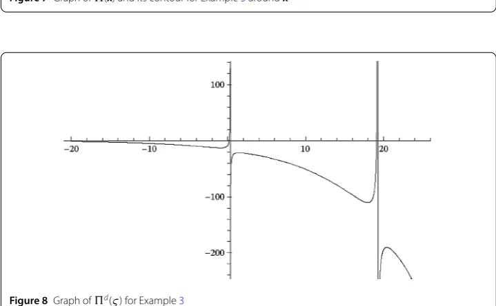
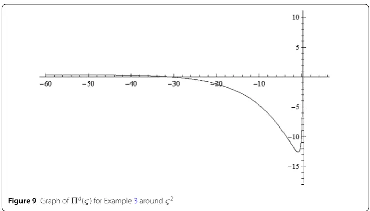
and from its graph, we can see clearly that it has five critical points in total (see Figs.8–9). These critical points can be easily obtained by Mathematica:

ς1= 20.396 >ς2= 17.9735 >ς3= 1.46219 >ς4= –0.881733 >ς5= –52.7144.

By Theorem1, we have all the primal solutions:

x1=

–21.57 16.065

, x2=

18.937 –13.93

, x3=

2.130 0.008

,

x4=

0.546 –1.797

, x5=

0.323 –0.272

.

Figure 6Graph of(x) and its contour for Example3aroundx1

Figure 7Graph of(x) and its contour for Example3aroundx2

Figure 8Graph ofd_{(ς) for Example3}

Figure 9Graph ofd_{(ς) for Example3aroundς}2

therefore,

S+

a ={ς∈R|ς> 19.266}, Sa–={ς∈R|ς< 0.367}.

By the facts thatς1∈S_a+andς5∈S_a–, we know that x1 is a globally stable fixed point,

x5_{is a locally unstable fixed point. Althoughς}4_∈S–

a is a local minimizer ofd(ς), we

cannot say if x4 _{is a locally stable fixed point sincedimX}

a= 2=dimSa = 1. But by the

complementary-dual principle and the order of the canonical dual solutions{ςi_{}, we have}

x1=dς1= –190.381

<x2=dς2= –110.759

<x3=dς3= –21.7036

<x4=dς4= –12.5735

<x5=dς5= 0.332915.

5 Conclusions

Based on the canonical duality theory, a unified model is proposed such that the general fixed point problems can be reformulated as a global optimization problem. This model is directly related to many other challenging problems in variational inequality, d.c. pro-gramming, chaotic dynamics, nonconvex analysis/PDEs, post-buckling of large deformed structures, phase transitions in solids, computer science, etc. (see [24] and the references cited therein). By the complementary-dual principle, all the fixed points can be obtained analytically in terms of the canonical dual solutions. Their stability and extremality are identified by the triality theory. Applications are illustrated by problems governed by non-convex polynomial, exponential, and logarithmic functions. Our examples show that both globally stable and locally stable/unstable fixed point problems inRn_{can be obtained}

eas-ily by solving the associated canonical dual problems inRm_{withm<n. However, the local}

and it deserves serious study in the future. Also, the results presented in this paper can be generalized to problems with nonsmooth potential functions.

Acknowledgements

The authors are thankful to the editors and the anonymous referees for their valuable comments, which reasonably improved the presentation of the manuscript.

Funding

The research was supported by US Air Force Office of Scientific Research under the grants (AOARD) FA2386-16-1-4082 and FA9550-17-1-0151.

Abbreviations

Not applicable.

Availability of data and materials

Data sharing not applicable to this article as no datasets were generated or analyzed during the current study.

Competing interests

The authors declare that they have no competing interests.

Authors’ contributions

All authors contributed equally and significantly in writing this article. All authors read and approved the final manuscript.

Publisher’s Note

Springer Nature remains neutral with regard to jurisdictional claims in published maps and institutional affiliations.

Received: 25 January 2018 Accepted: 25 September 2018

References

1. Anorld, V.I.: On teaching mathematics. Russ. Math. Surv.53(1), 229–236 (1998)

2. Ali, E., Gao, D.Y.: Improved canonical dual finite element method and algorithm for post-buckling analysis of nonlinear gao beam. In: Gao, D.Y., Latorre, V., Ruan, N. (eds.) Canonical Duality Theory: Unified Methodology for Multidisciplinary Study, pp. 277–290. Springer, New York (2017)

3. Bierlaire, M., Crittin, F.: Solving noisy, large-scale fixed-point problems and systems of nonlinear equations. Transp. Sci.

40, 44–63 (2006)

4. Border, K.C.: Fixed Point Theorems with Applications to Economics and Game Theory. Cambridge University Press, New York (1985)

5. Chen, Y., Gao, D.Y.: Global solutions to nonconvex optimization of 4th-order polynomial and log-sum-exp functions. J. Glob. Optim.64(3), 417–431 (2016)

6. Ciarlet, P.G.: Linear and Nonlinear Functional Analysis with Applications. SIAM, Philadelphia (2013) 7. Eaves, B.C.: Homotopies for computation of fixed points. Math. Program.3, 1–12 (1972)

8. Gao, D.Y.: Nonlinear elastic beam theory with applications in contact problem and variational approaches. Mech. Res. Commun.23(1), 11–17 (1996)

9. Gao, D.Y.: General analytic solutions and complementary variational principles for large deformation nonsmooth mechanics. Meccanica34, 169–198 (1999)

10. Gao, D.Y.: Pure complementary energy principle and triality theory in finite elasticity. Mech. Res. Commun.26(1), 31–37 (1999)

11. Gao, D.Y.: Duality Principles in Nonconvex Systems: Theory, Methods and Applications. Springer, New York (2000) 12. Gao, D.Y.: Analytic solution and triality theory for nonconvex and nonsmooth variational problems with applications.

Nonlinear Anal.42(7), 1161–1193 (2000)

13. Gao, D.Y.: Finite deformation beam models and triality theory in dynamical post-buckling analysis. Int. J. Non-Linear Mech.5, 103–131 (2000)

14. Gao, D.Y.: Canonical dual transformation method and generalized triality theory in nonsmooth global optimization. J. Glob. Optim.17(1/4), 127–160 (2000)

15. Gao, D.Y.: Sufficient conditions and perfect duality in nonconvex minimization with inequality constraints. J. Ind. Manag. Optim.1(1), 59–69 (2005)

16. Gao, D.Y.: Complete solutions and extremality criteria to polynomial optimization problems. J. Glob. Optim.35, 131–143 (2006)

17. Gao, D.Y.: Solutions and optimality to box constrained nonconvex minimization problems. J. Ind. Manag. Optim.3(2), 293–304 (2007)

18. Gao, D.Y.: On unified modeling, theory, and method for solving multi-scale global optimization problems. In: Sergeyev, Y.D., Kvasov, D.E., Mukhametzhanov, M.S. (eds.) Proceedings of the 2nd International Conference Numerical Computations: Theory and Algorithms. AIP Conference Proceedings, vol. 1776, 020005 (2016).

https://doi.org/10.1063/1.4965311

19. Gao, D.Y.: On unified modeling, canonical duality-triality theory, challenges and breakthrough in optimization. https://arxiv.org/abs/1605.05534(2016)

21. Gao, D.Y.: On topology optimization and canonical duality method. Comput. Methods Appl. Mech. Eng.341, 249–277 (2018)

22. Gao, D.Y.: Canonical duality-triality: Unified understanding modeling, problems, and NP-hardness in multi-scale optimization. In: Singh, V.K., Gao, D.Y., Fisher, A. (eds.) Emerging Trends in Applied Mathematics and Hi-Perfermance Computingy, Springer, New York (2018)

23. Gao, D.Y., Hajilarov, E.: Analytic solutions to 3-d finite deformation problems governed by St. Venant–Kirchhoff material. In: Gao, D.Y., Latorre, V., Ruan, N. (eds.) Canonical Duality Theory: Unified Methodology for Multidisciplinary Study, pp. 69–88. Spinger, New York (2017)

24. Gao, D.Y., Latorre, V., Ruan, N.: Canonical Duality Theory: Unified Methodology for Multidisciplinary Study. Advances in Mechanics and Mathematics, vol. 37. Springer, New York (2017).https://doi.org/10.1007/978-3-319-58017-3 25. Gao, D.Y., Ogden, R.W.: Multi-solutions to non-convex variational problems with implications for phase transitions

and numerical computation. Q. J. Mech. Appl. Math.61, 497–522 (2008)

26. Gao, D.Y., Ruan, N.: Solutions to quadratic minimization problems with box and integer constraints. J. Glob. Optim.

47(3), 463–484 (2010)

27. Gao, D.Y., Ruan, N., Latorre, V.: Canonical duality-triality theory: bridge between nonconvex analysis/mechanics and global optimization in complex systems. In: Gao, D.Y., Latorre, V., Ruan, N. (eds.) Canonical Duality Theory: Unified Methodology for Multidisciplinary Study, pp. 1–48. Springer, New York (2017)

28. Gao, D.Y., Ruan, N., Sherali, H.: Solutions and optimality criteria for nonconvex constrained global optimization problems with connections between canonical and Lagrangian duality. J. Glob. Optim.45, 473–497 (2009) 29. Gao, D.Y., Ruan, N., Sherali, H.D.: Canonical duality solutions for fixed cost quadratic program. In: Chinchuluun, A.,

Pardalos, P., Enkhbat, R., Tseveendorj, I. (eds.) Optimization and Optimal Control. Springer Optimization and Its Applications, vol. 39, pp. 139–156. Springer, New York (2010).https://doi.org/10.1007/978-0-387-89496-6_7 30. Gao, D.Y., Strang, G.: Geometric nonlinearity: potential energy, complementary energy, and the gap function.

Q. J. Mech. Appl. Math.XLVII(3), 487–504 (1989)

31. Gao, D.Y., Wu, C.: Triality theory for general unconstrained global optimization problems. In: Gao, D.Y., Latorre, V., Ruan, N. (eds.) Canonical Duality Theory: Unified Methodology for Multidisciplinary Study, pp. 127–154. Springer, New York (2017)

32. Gao, D.Y., Yu, H.F.: Multi-scale modelling and canonical dual finite element method in phase transitions of solids. Int. J. Solids Struct.45, 3660–3673 (2008)

33. Hirsch, M.D., Papadimitriou, C., Vavasis, S.: Exponential lower bounds for finding Brouwer fixed points. J. Complex.5, 379–416 (1989)

34. Huang, Z., Khachiyan, L., Sikorski, K.: Approximating fixed points of weakly contracting mappings. J. Complex.15, 200–213 (1999)

35. Jin, Z., Gao, D.Y.: On modeling and global solutions for d.c. optimization problems by canonical duality theory. Appl. Math. Comput.296, 168–181 (2017).https://doi.org/10.1016/j.amc.2016.10.010

36. Latorre, V., Gao, D.Y.: Canonical duality for solving general nonconvex constrained problems. Optim. Lett.10(8), 1763–1779 (2016).https://doi.org/10.1007/s11590-015-0860-0

37. Latorre, V., Gao, D.Y.: Global optimal trajectory in chaos and NP-hardness. Int. J. Bifurc. Chaos26, 1650142 (2016) 38. Liu, G.S., Gao, D.Y., Wang, S.Y.: Canonical duality theory for solving non-monotone variational inequality problems. In:

Gao, D.Y., Latorre, V., Ruan, N. (eds.) Canonical Duality Theory: Unified Methodology for Multidisciplinary Study, pp. 155–172. Springer, New York (2017)

39. Lu, X.J., Gao, D.Y.: Canonical duality method for solving Kantorovich mass transfer problem. In: Gao, D.Y., Latorre, V., Ruan, N. (eds.) Canonical Duality Theory: Unified Methodology for Multidisciplinary Study, pp. 105–126. Spinger, New York (2017)

40. Machalova, J., Netuka, H.: Control variational method approach to bending and contact problems for Gao beam. Appl. Math.62(6), 1–17 (2017).https://doi.org/10.21136/AM.2017.0168-17

41. Marsden, J.E., Hughes, T.J.R.: Mathematical Foundations of Elasticity. Prentice-Hall, New York (1983)

42. Ruan, N., Gao, D.Y.: Canonical duality approach for nonlinear dynamical systems. IMA J. Appl. Math.79, 313–325 (2014)

43. Scarf, H.: The approximation of fixed point of a continuous mapping. SIAM J. Appl. Math.35, 1328–1343 (1967) 44. Scarf, H.E., Hansen, T.: Computation of Economic Equilibria. Yale University Press, New Haven (1973)

45. Shellman, S., Sikorski, K.: A two-dimensional bisection envelope algorithm for fixed points. J. Complex.2, 641–659 (2002)

46. Shellman, S., Sikorski, K.: A recursive algorithm for the infinity-norm fixed point problem. J. Complex.19, 799–834 (2003)

47. Smart, D.R.: Fixed Point Theorems. Cambridge University Press, Cambridge (1980)

48. Voisei, M.D., Zalinescu, C.: Some remarks concerning Gao–Strang’s complementary gap function. Appl. Anal.90(6), 1111–1121 (2011)

49. Wang, Z.B., Fang, S.-C., Gao, D.Y., Xing, W.X.: Global extremal conditions for multi-integer quadratic programming. J. Ind. Manag. Optim.4(2), 213–225 (2008)