Augmenting camera images with gamma detector data

Peter A. von Niederhäusern

, Simon Pezold

, Uri Nahum

, Carlo Seppi

, Guillaume Nicolas

, Michael

Rissi

, Stephan K. Haerle

and Philippe C. Cattin

*Correspondence:

[email protected]

1_{Department of Biomedical} Engineering, University of Basel, CH-4123 Allschwil, Switzerland Full list of author information is available at the end of the article

Abstract

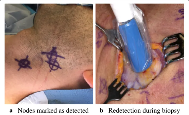
Background: Squamous cell carcinoma in the head and neck region is one of the most widespread cancers with high morbidity. Classic treatment comprises the complete removal of the lymphatics together with the cancerous tissue. Recent studies have shown that such interventions are only required in 30% of the patients. Sentinel lymph node biopsy is an alternative method to stage the malignancy in a less invasive manner and to avoid overtreatment. In this paper, we present a novel approach that enables a future augmented reality device which improves the biopsy procedure by visual means.

Methods: We propose a co-calibration scheme for axis-aligned miniature cameras with pinholes of a gamma ray collimating and sensing device and show results gained by experiments, based on a calibration target visible for both modalities.

Results: Visual inspection and quantitative evaluation of the augmentation of optical camera images with gamma information are congruent with known gamma source landmarks.

Conclusions: Combining a multi-pinhole collimator with axis-aligned miniature cameras to augment optical images using gamma detector data is promising. As such, our approach might be applicable for breast cancer and melanoma staging as well, which are also based on sentinel lymph node biopsy.

Keywords: Sentinel lymph node biopsy, Radioguided surgery, Augmented reality, Projective geometry, Multi-modality calibration

Background

Head and neck squamous cell carcinoma (HNSCC) is one of the most prevalent can-cers. Studies have shown that 70% of all HNSCC patients undergo overtreatment due to the limited accuracy of classic clinical and radiologic staging [1]. The specialist speaks of overtreatment if removal of unaffected lymph tissue is conducted. Sentinel lymph node biopsy (SNB) is the standard minimally invasive staging procedure for melanoma and breast cancer surgery and is currently validated in the domain of HNSCC treatment [2,3]. SNB is made possible by detecting gamma radiation from treated tissue. By injecting a technetium (99mTc)-based radioactive tracer, its uptake into the neighboring lymphat-ics can be measured by means of a gamma detector. Draining lymph nodes downstream of the tumor are amenable to acquire cancerous cells, and a biopsy of these identified

ceed, the surgeon obtains additional anatomic guidance from the preoperative assessment gained by SPECT/CT imaging. However, the crude intraoperative activity measurement makes it difficult for the specialist to target sentinel lymph nodes (SLNs). They are rather small and easy to miss (≈5 mm in diameter). It is consensus that lymph nodes with a high radioactivity foreground-to-background signal ratio are candidate sentinels [6]. A further complication is the distinction between the tracer accumulation at the injection site and those sentinel hot spots [7]. In HNSCC staging, this problem can be circumvented as the injection site is usually away from the biopsy site as the tracer is injected into the tongue. Inaccurate SNB staging due to missing SLNs would jeopardize the health of the patient and cause a disadvantage over classic ND treatment. Given these challenges of SNB, it is evident that intraoperative image-based 2D-to-2D visualization methods improve the procedure and remove the cognitive load for the surgeon (1D-to-3D, i.e., the need to correlate audio-based activity indication with anatomic structures).

One commercially available system for SNB, based on freehand SPECT (fhSPECT) and augmented reality (AR), is sold by the company SurgicEye (Munich, Germany) and was initially developed at TU Munich [8]. Freehand SPECT depends on a preparation and reg-istration step to align the tracked gamma probe with the patient. Gamma activity needs to be manually re-measured every time an update for the synthetic three-dimensional model

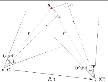
Fig. 2Schematic of a camera pair relation (exaggerated for illustrative purposes) with the corresponding projection of the world pointXonto the respective image planes,. The relative rotationRand translationtare known from calibration. The smallerRandt, the better the co-aligment between both cameras, making the overlay of their respective images possible

of the activity distribution is requested. Finally, this distribution model is displayed on an external monitor in the proximity of the surgeon which is not necessarily in their field of view [9]. The sequential nature of the procedure makes this approach rather involved for the operator.

Additionally, the IAEA provides an overview of current technologies and procedures of the field in the guided intraoperative scintigraphic tumor targeting (GOSTT)1report.

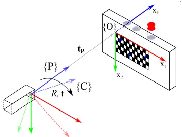
Fig. 3The pose of the pinhole wrt the target (solid arrows) is known. The pose of the target wrt the camera (dashed arrows) is determined by a pose estimation algorithm. Using the origin{O}as a pivot, we can calculate the rotationRand translationtfrom{P}to{C}. The tracer is contained inside the vial with the red cap. Exit pupils (blue circles) of the target are used to direct gamma radiation from the tracer for the image augmentation to assess the calibration

regime are seen under the same or similar viewing angle (Fig.8a). Thanks to the compa-rable opto-geometric arrangement of the cameras and the pinholes, projective geometry supports the image augmentation process, i.e., the embedding of additional information normally not seen, which is simpler and more direct than collecting and modeling a syn-thetic three-dimensional gamma activity distribution. Each of the four cameras can be used such that a specific augmentation with selective parameters is presented to the user. We recently published a feasibility study that showed how an augmentation of different modalities can be done, given a miniature camera that is axis-aligned with its harboring pinhole [10]. In this current paper we build upon the former and present the accompa-nying theoretical principles, why axis alignment supports the augmentation process even in the presence of a depth estimate and small alignment errors (“Methods and materials” section), and more varied experimental data showing the correspondence with respect to these governing principles (“Results” section). Finally, we discuss the achieved and provide thoughts about potential improvements and future applications of the method (“Discussion” section).

Methods and materials

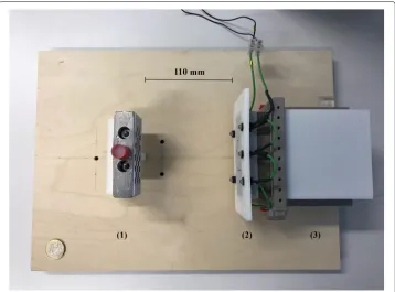
Fig. 4Calibration setup, viewed from the top. The stand with the calibration target and the vial (red cap) containing the tracer are placed on the left (1). The collimator with the attached camera fixation frame for the microscopic cameras and the LEDs (lighting) are to the right (2). The detector element is adjacent (3). The distance for this measurement is 110 mm from the collimator front plate to the target (calibration default). Not shown is the data processing unit of the detector. A 1-euro coin in the lower left serves as a scale reference

of the optical cameras with respect to their harboring pinholes, a calibration scheme, given in the “Calibration” section, is needed to assess these axis alignment differences. A depth prior of the gamma activity has to be determined to further improve the augmen-tation: a working distance of the detector to the activity inside the patient’s lymphatics needs to be estimated. For this to be valid, we assume isotropic radiation emission. The pose parameters (the position and orientation of a camera with respect to the origin) from the calibration are reused to obviate the need for a new ad hoc pose estimation

Fig. 6The camera on the left projects a known world point (X) onto its image plane (y˜). The difference₍px)

of the augmentation (yˆ), based on a depth estimate, is evaluated on the image plane (). The difference

(mm)of its reprojection(ˆˆX) is evaluated on a target plane (Q), given in world units (mm)

during each intervention. It is generally hard to accomplish this with sufficient accu-racy in a bright lit surgical setting, especially for cameras with low-resolution sensors. Thus, supportive error minimization schemes are needed and discussed in the “Error minimization schemes” section. The technical specifications of the collimator, the minia-ture endoscopic CMOS cameras and the detector are given in the “Hardware” section. The augmentation algorithm of the optical camera image with gamma information, based on these principles, is explained in theAppendix.

Foundation

The goal is to overlay a point that is seen by one pinhole camera, in our case the optical camera, with information from the other pinhole camera, in our case the gamma camera, when the configurations of the two cameras are known but not their distances to the projected world point, whose coordinates are given in relation to the origin. First, some definitions (cf.Fig.2):

a

b

Fig. 8aSingle pinhole of our multi-pinhole collimator, its field of view (2×α) defined by widthwand heighth. The wider field of view of the aligned camera is drawn in comparison.bRendering of the micro camera placement layout with respect to the pinholes (camera fixation frame not shown). The collimator is pointing towards the source (red arrow)

– Let{C}and{C}be the coordinate systems or frames of two cameras.

– LetXbe a point in 3D space, given byx=(x1,x2,x3)Tin{C}and

byx=(x₁,x₂,x₃)Tin{C}, respectively, wherex3,x3give the values along the

optical axes of the respective cameras (i.e., the distance or “depth”).

– LetT be the transformation from{C}to{C}, that is

x

1

=T

x

1

, (1)

where

T =

R t

0 1

(2)

with the3×3rotational partR=[ρ1|ρ2|ρ3]T(i.e.,ρ.form the rows (!) ofR ) and

translational partt=(t1,t2,t3)T, both known from the calibration step

(“Calibration” section).

Fig. 10 Pair 1, known source distance 90 mm (x3), acquisition time 16 s.aActivity image.bThe activity

accumulation (orange) of the source near the exit pupil (blue circle) of the CerrobendTM_{block is shown}

– Lety=(y1,y2)Tandy=(y₁,y₂)Tbe the points on the respective image planes in

the units of the world coordinates (i.e., mm, units of the calibration target) and let

˜

y= 1

f y and y˜

₌ 1

fy

₍₃₎

withy˜=(˜y1,˜y2)Tandy˜=y˜₁,y˜₂Tbe these very plane coordinates, normalized by

the respective focal lengthsf,f, both intrinsic parameters known.

– LetIdbe thed×didentity matrix.

Making use of the intercept theorem, we observe that for camera{C}, the following equalities hold (assumingf >0,x3>0):

⎛ ⎜ ⎝

y1

y2

f

⎞ ⎟

⎠= f

x3 x

(4)

⇐⇒

⎛ ⎜ ⎝

˜

y1 ˜

y2 1

⎞ ⎟

⎠= 1

x3 x

, (5)

⇐⇒x3

⎛ ⎜ ⎝

˜

y1 ˜

y2 1

⎞ ⎟

⎠= x, (6)

Fig. 11 Pair 2, known source distance 110 mm (x3), acquisition time 8 s.aActivity image.bGamma rays

Fig. 12 Pair 3, known source distance 130 mm (x3), acquisition time 16 s.aActivity image.bThe exit pupil

and the activity blob show slight discrepancies

and likewise for{C}(assumingf>0,x₃>0):

⎛ ⎜ ⎝

˜

y₁

˜

y₂ 1

⎞ ⎟

⎠= 1

x₃ x

_{. (7)}

Let us now assume that we measurey˜(or rather:y, which immediately gives usy˜) for the pointXin{C}’s camera plane and that we want to determine the respectivey˜in{C}’s camera plane, solely based on that measurementy˜. Let us therefore express{C}’s world coordinates in terms of{C}—which we can do by making use of Eq. (1)—and insert in Eq. (7), which gives us

⎛ ⎜ ⎜ ⎜ ⎝ ˜

y₁

˜

y₂ 1 1 ⎞ ⎟ ⎟ ⎟ ⎠= ₁

x₃I3 0

0 1 T x 1 . (8)

Now let us insert Eq. (6), that is,{C}’s image plane coordinates, on the right:

⎛ ⎜ ⎜ ⎜ ⎝ ˜

y₁

˜

y₂ 1 1 ⎞ ⎟ ⎟ ⎟

⎠=ScT Sc

⎛ ⎜ ⎜ ⎜ ⎝ ˜ y1 ˜ y2 1 1 ⎞ ⎟ ⎟ ⎟ ⎠ (9)

Fig. 13 Pair 4, known source distance 150 mm (x3), acquisition time 16 s.aActivity image.bThe exit pupil

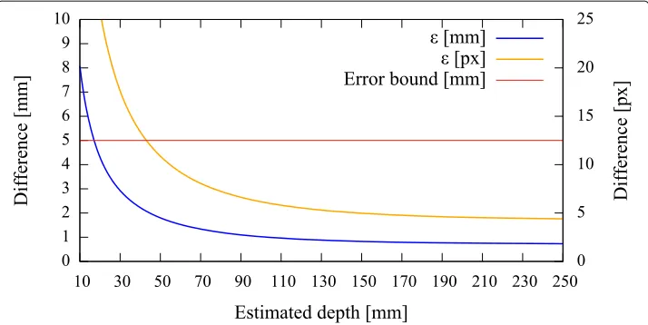
Fig. 14 Pair 1, true source distance 90mm (x3), initial camera distance 90.8 mm (x3). The curves(mm),₍px)

indicate that we are below the maximally allowed error in case the stored initial calibration is used (no automatic pose estimation). However, no apparent minimum is reached in the range of the depth estimates. Depending on the quality of the initial co-calibration at 110 mm, such effects are to be expected

with

Sc =

₁

x₃ I3 0

0 1

, Sc=

x3I3 0

0 1

. (10)

We denoteSc andScscaling matrices(cf.Eq. (7)) and above Eq. (9) can equivalently be written as

˜

y= x3

x₃Ry˜+

t

x₃. (11)

Fig. 15 Pair 2, true source distance 110 mm (x3), initial camera distance 109.8 mm (x3). Without automatic

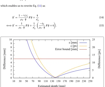
Fig. 16 Pair 3, true source distance 130 mm (x3), initial camera distance 124.9 mm (x3). The error curves

show their minima at≈140 mm

Here, we realize that we can expressx3in terms ofx₃via Eqs. (1)+(6). In particular, we may write

x₃=x3ρ3· ˜y+t3 (12)

⇐⇒x3=

x₃−t3

ρ3· ˜y , (13)

which enables us to rewrite Eq. (11) as

˜

y= 1−t3/x

3

ρ3· ˜y Ry˜+ t

x₃ (14)

⇐⇒ ˜y= 1

ρ3· ˜yRy˜+

1 x₃

−t3

ρ3· ˜yRy˜+t

. (15)

Fig. 17 Pair 4, true source distance 150 mm (x3), initial camera distance 150.3 mm (x3). The augmentation

Fig. 18 Backside view of the real collimator. Each pinhole yields an activity patch according to its

compartment. These compartments define the field of view of the pinholes. Some light-passing pinholes can be seen in the middle

Approximatingy˜without knowing x₃

In Eq. (15), onlyx₃remains unknown, which, in turn, only affects the right term of the equation. Assuming the right term was zero, we could exactly expressy˜in terms ofy˜, namely

˜

y= 1

ρ3· ˜yRy˜. (16)

For approximatingy˜without knowingx₃, we can thus try tochange our camera setupso that we minimize the right term of Eq. (15), making Eq. (16) a good approximation ofy˜. We have two options for this:

Fig. 20 Some error cases. The exposure time for these measurements is 16 s.aOverestimating the true distance: estimated distance 150 mm, the augmentation is slightly off.bUnderestimating the true distance: estimated distance 110 mm, the discrepancy is visible.cPathologic case: a ghostly (false) augmentation in the foreground due to high scattering not properly filtered

1. Simultaneouslymoving the cameras away from the imaged point X in the

direction of{C}’s optical axis or vice versa, leavingT unchanged, thus

x₃→ ∞ ⇐⇒1/x₃→0=⇒ 1 x₃

−t3 ρ3· ˜yRy˜+t

→0. (17)

2. Minimizing the distance|t|between the cameras while keeping the distancex₃, by

moving{C}as close as possible to{C}, thus

|t| →0=⇒[−t3→0andt→0]=⇒ 1 x₃

₋

t3 ρ3· ˜yRy˜+t

→0.

We have a third option to get a good approximation fory˜ without knowingx₃, even without changing our camera setup: in Eq. (15), we canuse a reasonable estimatexˆ₃in place ofx₃(i.e.xˆ₃≈x₃), giving us an estimateyˆfory˜, namely

ˆ

y= 1

ρ3· ˜yRy˜+

1 ˆ

x₃

₋

t3

ρ3· ˜yRy˜+t

≈ ˜y. (18)

Note that all three options may be combined.

Estimation error

The estimation error = ˆy− ˜yis given by

=

1 ˆ

x₃ − 1 x₃

−t3 ρ3· ˜yRy˜+t

(19)

or written for its componentsi(i=1, 2):

i=

1 ˆ

x₃ − 1 x₃

−t3ρi· ˜y

ρ3· ˜y +ti

. (20)

Note that using options 1 and 2 only or simply ignoring the right term of Eq. (15) corre-sponds to estimatingxˆ₃at infinity; thus,1/ˆx₃=0 in Eqs. (19)+(20).

– Let{O}be the world coordinate system’s origin defined by a planar target. This target is the frontal plane of a Cerrobend block with exit pupils for gamma radiation to escape in a directed manner (point source).

– Let{P}be the coordinate system of the pinhole.

– Let{C}be the coordinate system of the camera.

– LetXobe a list of known world points of the target, given byx=(x1,x2,x3)T

and∀x∈Xo: x3=0, in world coordinates.

– LetYcbe the projections ofXo, as detected by the optical camera, in camera image

(buffer) coordinates.

– LetKcbe the given internal parameters of the optical camera (e.g., focal length).

– LetRo,to=pose(Xo,Yc,Kc)be a pose estimation algorithm of{O}in{C}.

This algorithm is based on the functionsolvePnPof the computer vision

framework OpenCV [11].

Let us now assume that we spatially measure{P} solely in terms of{O}. This can be done as we know the relative position of the pinholetpwith respect to the target origin

{O}during calibration. As the pinhole’s image plane is perpendicularly aligned with the target (cf.Fig.4), and a pinhole is part of the rigid structure of the collimator frame and thus rotation free, we are allowed to setRp=I3and form the matrixPas

P=

I3 tp

0 1

, (21)

which transforms from{O}to{P}.

This is contrary to the unknown pose (i.e., position, orientation) of the optical cam-era with respect to{O}, due to rotations, tilts, and small offsets from the manufacturing process of the device. Let us assume that we measure allXoand match them with the pro-jectionsYc. The function pose(Xo,Yc,Kc)then yields the relative measurementsRc,tcof

the target in{C}, i.e., the mapping from{O}to{C}. In analogy to Eq. (21), we obtain the matrixCas

C=

Rc tc

0 1

. (22)

To get the complete transformation from{P}to{C}, we simply write

R,t=T =CP−1. (23)

section.

Error minimization schemes

Recall the goal to overlay optical camera images with gamma activity from the detector. These two modalities must therefore be joined. If for both the camera and the pinhole their spatial relation is known, and they identify thesameprojected world point (target), we know how to transfer information from one to the other (Fig.2). This corresponds to a homography formulation between the two sensors. On the other hand, the placement of the sensors can be chosen freely, given again that their relative spatial relation is deter-mined, if and only if we knew exactly the distance(s) from either sensor to the target. This corresponds to solving Eqs. (12), (13), and by consequence Eq. (11) and is a more restric-tive formulation of the above general homography. Neither of the two methods can be fully applied in our case by nature of the different modalities of the sensors. We therefore introduce axis alignment as a restriction.

Axis alignment

In the “Foundation” section, we propose three possible options to control the augmen-tation error, and we conclude that axis alignment is the most viable one: moving the camera/pinhole pair away too far from the target decreases the probability of gamma pho-tons, governed by the inverse square law, to reach the collimator and to trigger a signal on the detector. Furthermore, the focal length of the camera does only allow for a certain distance range to produce reasonably sharp images. As there isneithera unique target identification possible (for a potential homography), given the different modalities of the sensors, nor an exact distance measurement available, axis alignment helps to reduce the augmentation error. This is even more important if the activity does not coincide with the optical axes. A good depth estimate compensates for small misalignments of the axes (Fig.5).

New scaling matrices

Our approach needs to be flexible enough to handle variations in the placement of the device, thus also the camera/pinhole pairs, in relation to the radioactive source.

performance of the method at the system boundaries.

Error quantification

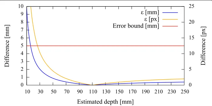
To be able to give a quantitative measure, we first modeled the effect of axis misalign-ment in the presence of a depth estimate (cf.Fig.6). Depending on the pose and location of the camera with respect to the pinhole, and the accuracy of the estimate, the differ-ences between theknownprojection of the world point and itsestimatedprojection and reprojection are evaluated each using theL2norm to give rise to the metrics (errors)(px)

and(mm)(Fig.7). The error(px)is calculated as the disparity between theknown pro-jection of a world point (i.e., the center of the exit pupil) onto the camera sensor and the transformation of that world point (i.e., the center of the activity blob) from the pinhole sensor onto the camera sensor according to Eq. (19) in pixel space. Furthermore, as it is relevant to the surgeon to know how far off from the actual lymph node they will initially place and drive the biopsy tools, theestimatedaugmentation is reprojected and compared with the world point in world units (mm) and its error expressed as₍mm). Note that in

Fig.6we omit the drawing of the pinhole and show the already transformed activities. To calculate this reprojection, we proceed as follows and use the notation from the sections above.

– LetXbe the known world point (true source location).

– Lety˜be the projection of the world point onto the image plane.

– Letyˆbe the augmentation, based on a depth estimate.

– LetXˆˆbe the reprojection ofyˆto yield the virtual source location.

– Let{C}be the coordinate system of the camera.

The augmentation yˆ is calculated according to Eq. (18). To get Xˆˆ, we find a planeQ whose normal vectorn= (n1,n2, 1)T is parallel to the linel(the reprojection) through the origin of{C}andyˆ. We then find the intersection of this line with the plane to get the virtual source location in the coordinate system defined by{C}. The planeQis defined as

Q:

⎛ ⎜ ⎝

p1−x1

p2−x2

p3−x3

⎞ ⎟ ⎠· ⎛ ⎜ ⎝ n1 n2 1 ⎞ ⎟ ⎠= ⎛ ⎜ ⎝

p1−x1

p2−x2

p3−x3

⎞ ⎟ ⎠· ⎛ ⎜ ⎝ ˆ

y₁

ˆ

y₂ 1

⎞ ⎟

⎠=0 (24)

wherep=(p1,p2,p3)T are points on the plane. The linelthrough the origin of{C}andyˆis given by

l: Co+λ

⎛ ⎜ ⎝

ˆ

y₁

ˆ

y₂ 1

⎞ ⎟

⎠=λ

⎛ ⎜ ⎝

ˆ

y₁

ˆ

y₂ 1

⎞ ⎟

The coordinates ofXˆˆ in the coordinate system of{C}are thus given by

ˆˆ

X=λYˆ= X

_{· ˆY}

Yˆ2

ˆ

Y. (27)

Error curves for varying depth estimatesxcan then be constructed. We also introduce an upper error bound to assess. As the resulting augmentation needs to be as close as possible to the center of the true source location (i.e., a lymph node, diameter≈5 mm), we do not tolerate augmentation errors larger than 5 mm (Fig.7). Furthermore, as the error can only be properly evaluated during calibration, the curves need to be read as an expected augmentation error with respect to the estimated (unknown) depth.

Hardware

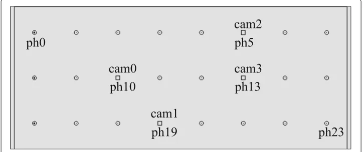
The design and layout of our multi-pinhole collimator are shown in Figs.8and9. This collimator is a tungsten-based device with a specific field of view, given the width and length of its pinhole compartments (Fig. 18). Each such evaluated compartment of a camera/pinhole pair is marked on the gamma sensor image in the “Results” section accordingly. The thickness of the front plate (1 mm) and the length of the septa (com-partment walls, 35 mm) are calculated such that the probability of background photons to penetrate the shields is at most 5%. The dimensions of the collimator frame are 86 mm in width, 36 mm in height, and 37 mm in depth. Its weight is 300 g.

In this study, we used endoscopic cameras (model NanEye, AMS AG, Premstätten, Austria) that measure 1 mm×1 mm×1.7 mm in width, depth, and height, respectively. Their resolution is 250×250 pixels with a pixel size of 3μm×3μm, and thus, an aspect ratio of 1:1. The effective focal length is 660μm. The built-in optics are wide-angle lenses with anf-number of 2.7, an aperture of 244μm, and an optimal focus range of 8–75 mm. The cameras are mounted and fixed on an 3D printed frame (ABS) matching the pinholes of the collimator. Thanks to this mounting, the cameras are mechanically constrained such that their lateral movement cannot exceed 0.5 mm and the distance to the pinholes is kept at a maximum of 3.0 mm (cf.Fig.4). As the optical cameras are exposed to high energy photons, a deteriorate effect might be expected. However, we did not observe any negative impact on the performance of the sensors over the course of our experiments.

photons (scatterers) is spread over the sensor area and impairs the augmentation.

Results

The figures in this section show different augmentation results during calibration and in situ measurements. The activity blobs are colored based on a heat map according to their radiation intensity; high photon counts yield brighter colors. All measurements show results from one gamma source (vial) with an activity of≈60 MBq. The vial is vari-ably positioned at three corresponding exit pupils of the calibration target. The detector exposure time is indicated for each figure. All camera/pinhole pairs are shown for tracer positions suitable for their respective field of view; we refer to each pair according to the naming scheme of Fig.9.

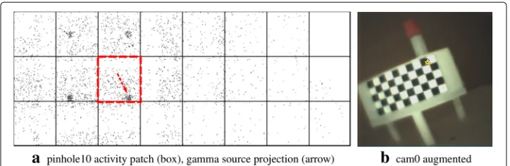
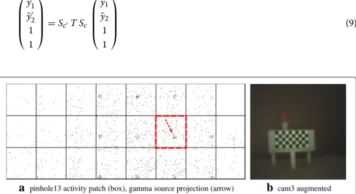
In Figs.10,11,12, and13, we present different detector activity images with associated pinhole (ph) patches (left) and corresponding augmentation results (right) based on auto-matic pose estimation. The respective exit pupil of the target is represented as a blue circle (unscaled for better visibility) with radius 1.5 mm, and the known distance(x3)from the pinhole to the target/source is indicated accordingly. These visualizations help to assess the calibration quality. In Figs.14,15, 16, and 17, the generated error curves(mm),(px)

(disparities) are based on the stored calibration from the previous figures, without auto-matic pose estimation and using depth estimates in the range 10–250 mm. Based on the true initial source distance(x3), the initial camera distance (x₃,cf.Eq. (12)) is also given. These curves allow a quantitative evaluation of the estimate as well as the initial co-calibration. In our case, the relevant curve is given by₍mm)(cf.“Error quantification”

section).

In Fig.19, we reuse the stored calibration parameters on a target with a different exit pupil layout compared to the calibration target and without a pattern for pose estima-tion. However, the distances are known (indicated). The exit pupils with a smaller radius of 0.5 mm are visible as darkish spots. Activities are shown at or near the exit pupils. No further visual indication is given, and the error plots omitted. Figure20a, b, and c represent images with augmentation errors. The first two images undergo augmentation with a deliberately wrong depth estimate to show the effect. The consequence of insuffi-cient thresholding or filtering to truly identify a landmark feature is shown as a pathologic case in the third image.

Discussion

In the case of HNSCC, the injection site is usually located at the tongue and thus away from the biopsy site. The discrimination of active over- and underlying tissue (so-called warm background) and potential sentinel nodes can be supported by inspecting the actual anatomy in case of an incision. However, for the initial placement of the biopsy tools in such an environment, or in case lymph nodes are positioned exactly above and below each other, specific targets need to be designed and tested with our method. Low activ-ity deposits of the initially injected doses in the lymphatics and tracer absorbing layers are other difficulties. As we do not have real-time update requirements, increasing the integration time of the device to collect more photons, and thus to get a better signal-to-background ratio, remedies these problems. Building an improved collimator to constrain unwanted background photons is an important next step. Device integration is in strong focus of the development. Challenges in image processing remain to properly filter and display the true activities (i.e., sentinel lymph nodes). Furthermore, the quality of the aug-mentation depends not only on a good initial joint calibration but also on mechanical stability and the exactitude of the assembly process (e.g., axis alignment). Nevertheless, even with limited micro-manufacturing abilities (some cameras exhibit pronounced rota-tions and tilts), the augmentarota-tions remain below or near our defined error bound. This shows the flexibility of the method. Finally, more synthetic tests with specific phantoms and different dosages as well as in vivo animal experiments need to be conducted to assess the sensitivity of our approach.

Conclusions

The strong dependence on preoperative imaging and the rather basic intraoperative ori-entation provided by one-dimensional audio-based gamma detectors are limiting factors for the successful application of sentinel lymph node biopsy (SNB). In HNSCC, a more targeted SNB enables a more reliable post-operative histopathologic staging, and there-fore a more effective analysis of potential tumor spreading. Breast cancer and melanoma staging based on SNB face similar challenges. Our approach might therefore also be applicable in these domains and could provide a step forward for SNB in general.

Endnote

1 http://www-pub.iaea.org/books/IAEABooks/10661/Guided-Intraoperative-Scintigraphic-Tumour-Targeting-GOSTT

Appendix

IV. Augmentation algorithm

flip patch vertically

for x←0 to rows−1 of patch for y←0 to columns−1 of patch

pixel←(x, y, 1)T

%from pinhole buffer coords to pinhole image plane coords pixel←K−1_p ·pixel

%apply transformation steps cpixel←Sc T Sp·pixel

%from camera image plane coords to camera buffer coords cpixel←Kc·cpixel

%perspective projection (homogeneous normalization) cpixel← _cpixel1₍₂₎·cpixel

%get activity color acc. to photon count at position x, y color←CLUT(patch(x, y))

%overwrite camera pixel with activity color img(cpixel, color)

endfor endfor

Abbreviations

99mTc: Technetium 99m (nuclear medicine radioactive tracer); ABS: Acrylonitrile butadiene styrene 404 (3d printing material); AR: Augmented reality; CMOS: Complementary metal-oxide-semiconductor; cN0-neck: Clinically negative neck; fhSPECT: Freehand single photon emission computed tomography; GOSTT: Guided intraoperative scintigraphic tumor targeting; HNSCC: Head and neck squamous cell carcinoma; IAEA: International Atomic Energy Agency; ND: Neck dissection; SLN: Sentinel lymph node; SNB: Sentinel lymph node biopsy; SPECT/CT: Single photon emission computed tomography/computed tomography

Acknowledgements

We would express our gratitude to Dr. Goetz Kohler from the University Hospital Basel, Clinic of Radiotherapy & Radiation Oncology, for manufacturing the Cerrobend calibration targets.

Funding

This study is supported by the Gebert Rüf Foundation, Basel, Switzerland. This founding body doesnottake part in any of the following: the design of the study and collection, analysis, and interpretation of data and in writing.

Availability of data and materials

The datasets used and/or analyzed during the current study are available from the corresponding author on reasonable request.

Authors’ contributions

Not applicable.

Consent for publication

Not applicable.

Competing interests

The authors declare that they have no competing interests.

Publisher’s Note

Springer Nature remains neutral with regard to jurisdictional claims in published maps and institutional affiliations.

Author details

1_{Department of Biomedical Engineering, University of Basel, CH-4123 Allschwil, Switzerland.}2_{University Hospital Basel,}

Radiology & Nuclear Medicine Clinic, CH-4031 Basel, Switzerland.3DECTRIS Ltd., CH-5405 Baden-Dättwil, Switzerland.

4_{Center for Head and Neck Surgical Oncology and Reconstructive Surgery, Hirslanden Clinic, CH-6006 Lucerne,}

Switzerland.

Received: 28 November 2018 Accepted: 6 May 2019

References

1. Coskun HH, Medina JE, Robbins KT, Silver CE, Strojan P, Teymoortash A, et al. Current philosophy in the surgical management of neck metastases for head and neck squamous cell carcinoma. Head Neck. 2015;37(6):915–26. 2. Calabrese L, Bruschini R, Ansarin M, Giugliano G, De Cicco C, Ionna F, et al. Role of sentinel lymph node biopsy in

oral cancer. Acta Otorhinolaryngol Ital: organo ufficiale della Societ˙a italiana di otorinolaringologia e chirurgia cervico-facciale. 2006;26(6):345–9.

3. Radkani P, Mesko TW, Paramo JC. Validation of the sentinel lymph node biopsy technique in head and neck cancers of the oral cavity. Am Surg. 2013;79(12):1295–7.

4. Tsuchimochi M, Hayama K. Intraoperative gamma cameras for radioguided surgery: technical characteristics, performance parameters, and clinical applications. Phys Med. 2013;29(2):126–38.

5. Govers TM, Hannink G, Merkx MAW, Takes RP, Rovers MM. Sentinel node biopsy for squamous cell carcinoma of the oral cavity and oropharynx: a diagnostic meta-analysis. Oral Oncol. 2013;49(8):726–32.

6. Moncayo VM, Aarsvold JN, Alazraki NP. Lymphoscintigraphy and sentinel nodes. J Nucl Med. 2015;56(6):901–7. 7. Haerle SK, Stoeckli SJ. SPECT/CT for lymphatic mapping of sentinel nodes in early squamous cell carcinoma of the

oral cavity and oropharynx. Int J Mol Imaging. 2011;2011:106068.

8. Wendler T, Herrmann K, Schnelzer A, Lasser T, Traub J, Kutter O, et al. First demonstration of 3-D lymphatic mapping in breast cancer using freehand SPECT. Eur J Nucl Med Mol Imaging. 2010;37(8):1452–61. 9. Okur A, Ahmadi SA, Bigdelou A, Wendler T, Navab N. MR in OR: First analysis of AR/VR visualization in 100

intra-operative freehand SPECT acquisitions. 2011 10th IEEE International Symposium on Mixed and Augmented Reality. ISMAR. 2011;2011:211–8.

10. von Niederhäusern PA, Maas OC, Rissi M, Schneebeli M, Haerle SK, Cattin PC. Augmenting scintigraphy images with pinhole aligned endoscopic cameras: a feasibility study. In: Zheng G, Liao H, Jannin P, Cattin P, Lee SL, editors. Medical Imaging and Augmented Reality. MIAR 2016. Lecture Notes in Computer Science, vol 9805. Cham: Springer; 2016. p. 175–85.

11. Bradski G. The OpenCV library. Dr Dobb’s J Softw Tools. 2000;25:120, 122–125.

12. Henrich B, Bergamaschi A, Broennimann C, Dinapoli R, Eikenberry EF, Johnson I, et al. PILATUS: a single photon counting pixel detector for X-ray applications. Nuclear Instruments and Methods in Physics Research, Section A: Accelerators, Spectrometers. Detectors Assoc Equip. 2009;607(1):247–9.