University
of
Bolton
Conferences
Research
and
Innovation
Conference
2012
University
of
Bolton
Year
2012
Automatic Absolute and Relative Camera Egomotion
Estimation based on Visual Features
Dominik Aufderheide *
Werner Krybus and Gerard Edwards†
* South Westphalia University of Applied Sciences, Division Soest, Germany, aufderheide@fh‐swf.de
South Westphalia University of Applied Sciences, Division Soest, Germany, krybus@fh‐swf.de
† University of Bolton, UK, [email protected]
This paper is posted at UBIR: University of Bolton Institutional Repository, and has not been amended or
Automatic Absolute and Relative Camera Egomotion
Estimation based on Visual Features
Dominik Aufderheidea,b, Werner Krybusa, Gerard Edwardsb
aSouth Westphalia University of Applied Sciences, Division Soest
Institute for Computer Science, Vision and Computational Intelligence Luebecker Ring 2, 59494 Soest, Germany
E-Mail: {aufderheide, krybus}@fh-swf.de
bThe University of Bolton, Faculty of Advanced Engineering and Sciences
Deane Road, Bolton BL3 5AB, U.K. E-Mail: {dma1bee, g.edwards}@bolton.ac.uk
Abstract
The automatic estimation of a cameras position based on visual measurements is a gen-eral problem in the field of computer vision. Based on the estimated cameras trajectory it is possible to solve common tasks, such as Visual Odometry (VO) in the field of mo-bile robotics or the automatic reconstruction of an observed scene, based on classical Structure-from-Motion (SfM) techniques. The general procedure of camera egomotion estimation is always based on visual feature tracking and subsequent Perspective-n-Point (PnP) camera pose determination. This article evaluates recent algorithms for camera egomotion estimation based on point feature correspondences for their applicability in VO applications. These algorithms use methods based on 2D/2D and 3D/2D correspon-dences and are assessed in experimental evaluations employing synthetic data sets. It was found that the accuracy of the evaluated techniques is predominantly influenced by the number of correspondences and underlying motion patterns. Additional routines such as outlier handling and key frame detection were found to be mandatory for real-world application.
Keywords: Camera egomotion estimation, Pose Estimation, PnP problem, SLAM, Structure from motion (SfM) PnP-problem
1. Introduction
Many applications in computer vision require an accurate estimate of the cameras position and orientation as a prerequisite for further computations (see Davison (2003), Maimone et al. (2007), Nistr et al. (2004) and Davison et al. (2007)). Prominent examples are applications from Augmented Reality (AR), Structure-from-Motion (SfM) or visual navigation. In this context also possibilities for the estimation of a robots position based on visual measurements are widely discussed. Here the term Visual Odometry (VO) was introduced for a class of methods which provide the possibility to estimate the motion of a moving robot platform by using visual sensors (see Nistr et al. (2004) and Maimone et al. (2007)). Closely related is the field of Simultaneous Localisation And Mapping (SLAM) which combines ideas from vision based motion estimation with a simultaneous
modelling of the robots environment (see Davison (2003) and Davison et al. (2007)). This paper evaluates recently proposed numerical methods for camera egomotion esti-mation based on point features for their applicability within 3D scene modelling. The remainder of this paper is organised as follows: Section 2 introduces a general frame-work for visual camera egomotion estimation and explains the different subtasks which have to be tackled. In this context pose estimation methods based on 2D/2D correspon-dences and 3D/2D corresponcorrespon-dences are treated separately. Both of them are explained in the subsequent sections 3 and 4. The results of an experimental evaluation is given in section 5. Finally section 6 summarises and concludes the whole paper and gives an outline of possible future work.
2. General Concepts in Camera Egomotion Estimation
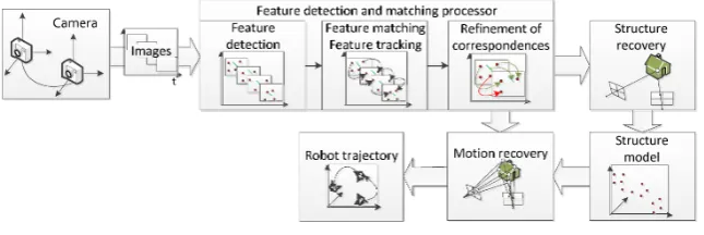
The general procedure of camera egomotion estimation based on a monocular image stream can be subdivided into different subtasks. The minimal configuration of a VO framework represented in the following figure contains three major subtasks: feature handling, structure recovery and motion recovery.
Figure 1: Minimal configuration for a methodology framework for visual odometry
The feature handling routine contains three distinctive phases beginning with the feature detection. Those features could be in various categories, however most schemes are based on point features, because the automatic identification of distinctive points (corners, junctions, etc.) is a well studied field in image processing. Most classical ap-proaches use Harris corners (see Harris and Stephens (1988)) but also recently published SIFT (Lowe (2004)) and SURF (Bay et al. (2008)) methodologies have drawn the at-tention of researchers. The matching of point features between successive frames is a problem which is often combined with feature tracking based on motion estimation. In this context Kalman or particle filtering have been used for rigid scenes, while the com-bination of classical Hidden Markov Models (HMM) and Gauss-Markov-Random-Fields (GMRF) have been employed for scenes including articulated objects (see Rehrl et al. (2010)).
As it was shown e.g. by Aufderheide et al. (2009) and Steffens et al. (2009a) the problem of feature tracking is unstable because there are numerous possibilities for the occurrence of wrong matches (outliers). In most cases a refinement of the correspondences is neces-sary neglecting any outliers.
The next stage to be considered is the motion recovery. Two different general techniques can be identified in literature for motion recovery (see Jiang et al. (2000)):
• 2D/2D correspondence between image features and subsequent estimation of
epipolar relations
• 2D/3D correspondence between image features and a scene model which
con-tains calibrated feature positions
The following two sections introduce both methodologies briefly.
3. Pose Estimation from 2D/2D Correspondences
The general problem of relative pose estimation based on a set of 2D/2D correspon-dences can be formulated as the recovery of time-varying parameters of a cameras ego-motionRk,tk from corresponding image feature coordinates [ui,k, vi,k]T. In this context
it is necessary to distinguish two different setups: the calibrated or uncalibrated camera setup.
The relative pose parametersRk,tk are directly related to the essential matrixEas
defined as follows:
Ek=Rk[tk]× (1)
In general for an image point in homogeneous coordinates ˜x= [u v1]T for image I
and an corresponding image point x˜0 = [u0v01]T
for image I0, the simplified epipolar constraint per the following equation is true:
˜
q0TE˜q= 0 (2)
Here ˜q and q˜0, the normalised camera coordinates, are computed by multiplication of the image points with the inverse of the predetermined calibration matricesK and K0
of the camera, according to Equation 3 below:
˜
q=K−1˜xandq˜0 =K0−1˜x0 (3)
The intrinsic calibration matricesKandK0are determined within a prior calibration routine.
One important constraint for estimation ofE is the fact that the matrix is singular:
det(E) =0 (4)
By using the additional constraint from Equation 4 it is possible to reduce the minimal number of points for estimatingE to be seven. It was shown in Philip (1996), that the additional property of the essential matrix, as shown in Equation 5, which can be derived from the fact that the two non-zero singular values ofEare equal, can be used to reduce the sufficient number of points to estimateEto be six (see Philip (1996)), and five (see Nist´er (2004)) respectively.
EETE−1
2trace
EETE= 0 (5)
It was shown in an experimental evaluation by Rodehorst et al. (2008) that the usage of five-point algorithms outperforms other techniques, especially for noisy data. Despite the conclusion in Br¨uckner et al. (2008), which suggested a combination of an eight-point and an five-point estimator as the optimal solution for robust relative pose, the current approach considers the five-point relative pose estimator as suggested by Nist´er (2004) for the sake of simplicity and computational efficiency.
3.1. Five point Relative pose estimation
The following section describes in part 3.1.1 how to calculateE from 2D/2D corre-spondences. Section 3.1.2 covers the recovery of the motion parametersRk,tk from the
essential matrix. In most cases the set of corresponding points will contain a significant number of wrong matches (outliers). Thus it is necessary to develop a strategy to handle outliers for generating robust estimates of the cameras egomotion. In the present work a guided-Random Sample Consensus approach, described in section 3.1.3, is adopted to handle the outliers problem.
3.1.1. Calculation of the essential matrix
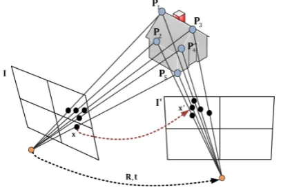
For a fully calibrated camera setup it was shown in the classical work Kruppa (1913) that at least five corresponding image features (here: points) in two frames of a sequences are necessary to recover the relative motion of the camera. The general setup of the relative pose problem is given below in Figure 2.
Figure 2: The 5-point relative pose problem with a house as the subject
Each pair of the corresponding points in the imagesxleads to one equation, following the constraint shown in Equation 2. Nist´er (2004) has suggested the formulation˜qTE˜=
0, with:
˜
q= x˜[1]˜x0[1] x˜[2]˜x[1]0 x˜[3]˜x0[1] x˜[1]˜x0[2] x˜[2]˜x0[2] ˜x[3]˜x0[2] ˜x[1]˜x0[3] ˜x[2]˜x0[3] ˜x[3]˜x0[3]
T ˜
E= E[1,1] E[1,2] E[1,3] E[2,1] E[2,2] E[2,3] E[3,1] E[3,2] E[3,3]
T
For all five point correspondences the following 5 x 9 data matrixQ˜ can be obtained: ˜ Q= ˜ q1
[1] · · · ˜q 1 [9] .. . ... ... ˜ q5
[1] · · · ˜q 5 [1]
(6)
The solution forE is found by first decomposingQ˜ by singular value decomposition (SVD) (see Br¨uckner et al. (2008)) or QR-factorisation (see Nist´er (2004)) to compute the null space. The null space leads to vectorsA˜,B˜,C˜ andD˜. Then the following linear combination of these vectors (A˜,B˜,C˜ andD˜) yields to the essential matrix:
E=a·A+b·B+c·C+d·D (7)
It should be noted that the four scalar values a,b,c and d are just defined up to a common scale, so it can be taken thatd= 1. Substituting Equation 7 into the constraints as shown in Equation 5 the problem can be formulated as the solution of ten polynomial equations of third degree. Nister suggested an algorithm for solving the problem to recover the unknowns of the system and recovering the essential matrixE, where up to ten solutions are possible. In recent years a variety of methods for the final estimation of E have been suggested in literature. The original algorithm proposed by Nister in Nist´er (2004) uses Sturm sequences to solve a univariate formulation of the problem. Later Stewenius et al. (2006) proposed a more efficient procedure based on Groebner bases. It was suggested by Kukelova et al. (2008) that a formulation as a polynomial eigenvalue problems is more straightforward and leads to solutions which are numerically more stable. These different methods were evaluated in terms of accuracy and robustness against noise in section 5.1.
In most cases the feature detection and matching routine will produce more than the minimum set of five correct point correspondences. In those cases, the ”best” solution can be found by evaluating a defined error metric.
Different kinds of error metrics are defined in literature. In Rodehorst et al. (2008), the Sampson error metricde over all matches `, is used, which should be minimal for the
correct solution ofEand can be defined as follows:
de= `
X
K=1
˜ xT
k0E˜xk
[E˜xk]2x+ [E˜xk]2y+ [ETx˜0k] 2
x+ [ET˜x
0
k] 2 y
(8)
Hartley and Zisserman (2004) uses the classic algebraic error based on the simpli-fied epipolar constraint as already defined in Equation 2. Another error metric is the symmetric squared geometric error, as suggested by Br¨uckner et al. (2008):
dssg =
˜ xTk0E˜xk
2
[E˜xk] 2
x+ [E˜xk] 2 y
+ x˜
T k0E˜xk
2
[ET˜x0
k] 2 x+ [E
T˜x0
k] 2 y
(9)
3.1.2. Recovering motion parameters
Once the essential matrix is known, the egomotion of the camera between two suc-cessive frames can be retrieved fromE. Note thatE can just be recovered up to scale. There is also an ambiguity, in that there are four possible solution pairs for the rotation
matrix and the translation vector.
The first step in determiningRand tfrom E is the computation of the singular value decomposition (SVD) of the essential matrix:
E ∼ UΣVT (10)
As it was shown in Hartley and Zisserman (2004) the four possible solution pairsR
and tcan be constructed from the two different solutions for the rotation matrix Ra,
Rb and two different solutions for the translationta, tb as follows: {Ra,ta}, {Rb,tb},
{Ra,tb} and{Rb,ta}.
The definition of the solutions is based on the following definitions forta andtb:
ta ≡ U[1,3] U[2,3] U[3,3]
T
; tb≡ −1· U[1,3] U[2,3] U[3,3]
T
(11)
Ra andRb are defined as follows:
Ra=UDVT; Rb=UDTVT (12)
with
D=
0 1 0
−1 0 0
0 0 1
This four-fold ambiguity can be resolved by using the cheirality constraint, which states that the observed feature points have to be located in front of both cameras. For this it is necessary to reconstruct the three-dimensional coordinates of at least one feature point by using standard triangulation methods and the four possible solutions for the motion parameters. It is only in one of these cases, where the reconstructed point lies in front of both cameras.
3.1.3. Guided-Random Sample Consensus for handling outliers
Usually the feature detection and matching routine will provide more than five cor-responding points between two successive frames of the image sequence. However, it is very likely that the set of point matches contains also a non negligible number of wrong matches (outliers). So there remains the open question of choosing the optimal point correspondences for the relative pose estimation.
Instead of employing a random sampling which would treats all samples equally, a guided sampling based on a-priori known measurements from the feature detection and match-ing procedure is used here. Here the general procedure, is based on ideas from Random Sample Consensus (RanSaC).
Most feature detection methods lead to a score which can be interpreted as kind of a distinctiveness measure1ξand also the matching procedure leads to a similarity measure
ρ. For the numerical experiments incorporating Harris features, the distinctivenessV[u,v]
1It should be stated that the general termdistinctivenessdescribes different properties for different
feature detectors. So the distinctiveness for a corner-detector would be labelled more exactly as ”cor-nerness” while the features extracted by Fast-Radial Symmetry Transform (FRST) (see Steffens et al. (2009b)) are selected based on their ”roundness”.
at the corner positions definesξ. These information sources are weighted by factorswξ
andwρ to compute an indicatorτ which can be interpreted as the likelihood for being a
correct or wrong match.
For the estimation ofE at least five matches are necessary. Hence, the minimal sample sets (MSSs) consist of five matches which are sampled from the set of matches pre-sorted with respect toτ. An iterative procedure is used to generate estimates forE from Nis-ter’s five-point algorithm, until a test of the actual configuration produces a Sampson errorde (see Equation 8) over all matches `, below a specified threshold dlim. Besides
that, the number of inliers produced by the actual configuration ofEis evaluated for the stop criterion. The whole procedure for estimating relative camera pose is described by the following Algorithm 1.
Algorithm 1Guided-RanSaC procedure for camera egomotion estimation
1: Detect n features inIand m features inI0 and computeξi:i∈ {1...n} andξ0j :j∈ {1...m}
2: Find` corresponding pointsqk andqk0 and computeρk withk∈ {1...`}
3: forall found matches` do
4: {Calculate likelihood for being a correct match}
5: τk=wξξk+wρρk
6: end for
7: Sort all found matchesxandx0 byτ
8: Transformxandx0 to normalised coordinatesqandq0 9: Sample N MSSs from sorted matches
10: while(de< dlim)∧(g≤N)∧(h > hlim)do
11: EstimateEwith MSS g:g∈ {1...N} 12: Calculatedeover` matches
13: Calculate number of inliers h with actualE
14: end while
15: ExtractRa,Rb andta,tb from Eby SVD
16: Chose correct solution forRandtby cheirality constraint
4. Pose Estimation from 3D/2D Correspondences
As already stated before, there is also the possibility to recover the egomotion of camera by means of 3D/2D correspondences. The following section summarises ideas for the estimation of absolute camera pose based on 2D/3D correspondences. The general idea is the successful tracking of anchor features of an initial scene model in the images of the monocular image stream. In this work we consider both partially or fully cali-brated setups, where in a fully calicali-brated setup the intrinsic camera calibration matrix
Kis known, while for partially calibrated setups the focal lengthf may vary during the sequence. This is especially relevant for zooming cameras, because the effective focal length will change considerably during the acquisition of the scene.
4.1. General introduction to the PnP-problem
The PnP problem can be described as the estimation of the absolute position and orientation of a camera based on a set of n 2D/3D correspondences between the image acquired by the camera and a three-dimensional scene model. It is also assumed that the intrinsic parameters of the cameras are at least partially known.
For the uncalibrated case, it was shown that at least six corresponding features have to be known to estimate the absolute pose of the camera and five inner calibration parameters (effective focal length (fu, fv), position of the principal point (u0, v0) and skewness of the
image axis (s)). For this configuration a linear solution exists and a method for solving the problem was published in the mid-seventies by Marzan and Karara (1975).
Recently different methods and algorithms have been proposed for the calibrated case. The major aim of the present investigation is the evaluation of different methodologies for real-time camera egomotion estimation for visual odometry:
• EPnP- Lepetit et al. (2009) suggested a non-iterative procedure forn≥4 based on the definition of four virtual control points. The given n 3D points are expressed as a weighted sum of these control points thus reducing the whole problem to estimating the control points, with respect to the camera coordinate system (CCS). This approach reduces the complexity of the problem toO(n).
• P4Pf - The procedure introduced in Bujnak et al. (2008) is an example for a methodology which is able to handle only partially calibrated setups, as the sug-gested algorithm has the capability of recovering the effective focal length of the camera. By usingn= 4, a minimal solution can be found based on Groebner basis techniques.
• P4Pfr - Finally the algorithm presented in Josephson and Byr (2009) estimates in addition the radial distortion which was neglected within the former schemes. It should be pointed out that the distortion coefficients for a radial distortion model are often calculated during the calibration of the camera. The use of a zooming camera however will involve the possibility of varying distortions. This method is also based on Groeber basis solvers and suggests the usage inside a RanSaC-scheme.
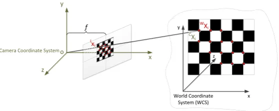
We tested theEPnP-approach, described in the following discussion, for this work: The general configuration of the PnP-problem, as shown in the Figure 3, consists of estimating the camera position, based on a given set of n image projections{Ix
i}ni=1 of
n general 3D reference points{WX
i}ni=1in the world coordinate frame.
The corresponding projection can be formulated in terms of the projection matrixP
as follows:
αiIxei=PWXei (13)
P contains information about the rigid transformation between the WCS and the CCS in terms of the rotation matrix R and the translation vector t and the intrinsic parameters of the camera. Here it is now important to discern the number of unknown variables of the camera matrixK. In the EPnPapproach all parameters are assumed to be known. TheP4Pf algorithm assumes a known calibration matrix up to the focal length and theP4Pfrprocedure includes also the assumption that the image points are
World Coordinate System (WCS) x y z x y z o Camera Coordinate System
f x W Xi Ix i C Xi
Figure 3: PnP problem
affected by radial distortion. Thus for the EPnP, P4Pf and P4Pfr techniques the number of degrees of freedom of the problem, which have to be solved for, is varying. If all elements ofKare well known and the influence of a radial distortion is neglected, there are six degrees of freedom; three translation parameters and three rotation angles. Thus, at least three 3D/2D correspondences need to be known to solve this problem (see the classical work of Grunert (1841) for a derivation). This is why this configuration is often labelled as P3P (see Gao et al. (2003)). The suggested approach from Lepetit et al. (2008) reformulates the classical P3P problem by introducing four virtual control points{WC
j}4j=1 which are used to describe the given n feature points:
g WX i= 4 X j=1
αi,jWgCj, with
4
X
j=1
αi,j= 1 (14)
The coordinates of{WC
j}4j=1 are chosen in the following manner:
WC
1 is chosen as
the centroid of the given n feature points andWC2,3,4forming a basis aligned with the
principal directions of the given data points.
By using the given correspondences the whole problem can be formulated as:
ωi Iu i Iv i 1 =
fu 0 uc
0 fv vc
0 0 1
4
X
j=1
αi,jCCj (15)
The last row of the system states thatωi= 4
P
j=1
αi,jCzj, whereCzjis the z-coordinate
ofCCj. ωiis a projective parameter, which can be substituted from the expression above
leading to two linear equations which can then be formulated for each given 3D/2D correspondence:
4
X
j=1
αi,jfuCxj+αi,j uc− Iui
Cz
j= 0
4
X
j=1
αi,jfuCyj+αi,j vc−Ivi
Cz
j = 0
(16)
The corresponding system of 2n equations can be solved by classical techniques from linear algebra, where the 12 coordinates of the chosen control points in camera coor-dinates have to be estimated. Lepetit et al. (2008) produce a closed-form solution for
n ≥ 4, where a subsequent and optional Gauss-Newton optimisation is carried out in order to increase the accuracy of the solution.
5. Results
We tested relative pose estimation from 2D/2D point correspondences and absolute pose estimation with PnP-algorithm based on 3D/2D correspondences by using synthetic data. This strategy provides a controlled environment for generating different motion patterns, testing the influence of noise and the typical number of outliers in the data set. The following section 5.1 summarises the experiments and results for evaluating relative pose estimation techniques, while section 5.2 describes visual odometry based on 3D/2D correspondences and its performance.
5.1. Relative pose estimation from 2D/2D correspondences
The whole procedure for relative camera pose estimation using Guided-RanSaC was evaluated based on both synthetic and real data sequences. In this context the different steps of the whole approach were observed separately.
The synthetic data was generated by defining a motion profile of a virtual mobile robot containing both rotational and translational movements. By using the standard pinhole-camera model as described e.g. in Hartley and Zisserman (2004), a randomly generated scene model is projected on virtual images of the scene at the different positions. Thus it is possible to generate pairs of corresponding image points as a basis for the evaluation. For the different time steps, it is possible to add noise to the point coordinates or generate additional non-correct matches (outliers).
It is necessary to define a procedure for a numerical evaluation of the performance of the different algorithms. In this context two different error metrics are defined inspired by ideas from Br¨uckner et al. (2008):
• Translation error -et: Due to the fact that the camera egomotion parameters can
only be recovered up to an arbitrary scale the translation error is measured by the angle between the ground truth translation vectortand estimated onete:
et=arccos
_ te·
_
t= arccos
te
|te|
· t
|t|
(17)
• Rotation error -er: Three unit vectorsex,eyandezare rotated using the original
(Rgt) and the estimated rotation matrixRe. The error metric is defined as follows:
er=
1 3
X
i∈{x,y,z}
arccos(Rgtei) T
Reei
(18)
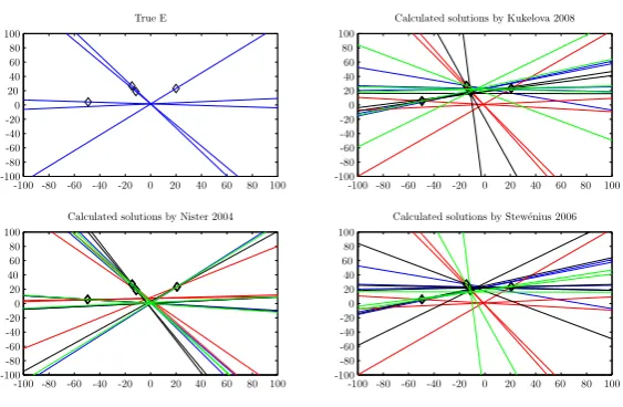
Figure 4 gives results for the estimated epipolar geometries from the true solution and three different algorithms. Here the different four sub figures display the epipolar linesI→ I0, as calculated by Equation 19, for the four different solutions provided by different algorithms for a given true solution. The upper left sub figure shows the correct configuration. Then the polynomial eigenvalue approach, labelled ’Kukelova’ in the figure from Kukelova et al. (2008), the method using Sturm sequences, labelled ’Nister’ in the figure, as suggested by Nist´er (2004), and the solution based on Grobner bases, labelled ’Stewenius’ in the figure, introduced by Stewenius et al. (2006) are placed sequentially row by row in the overall figure. The image coordinates for the visualisation are normalised between [−100,100].
I→I0:l0=Eq (19)
Figure 4: Estimated epipolar lines of the generated solutions from the true solution and three different algorithms (Kukelova, Nister, Stewenius) for the five-point relative pose problem
To evaluate the two different algorithms 100 random point sets were generated and the rotation and translation error, as defined above, were determined. The whole procedure was repeated for different levels of noise. The first approach selects the best solution from both algorithms based on the a-priori known true solution forE, which provides the possibility to evaluate only the algorithm itself. For a second test the different error metrics (algebraic error, symmetric squared geometric error and Sampson distance) for chosing the best solution are incorporated in the evaluation. By using different error metrics, it is possible to choose the best combination of estimator and error metric in terms of robustness and accuracy. The correct solutions for R and t are chosen by following cheirality constraint.
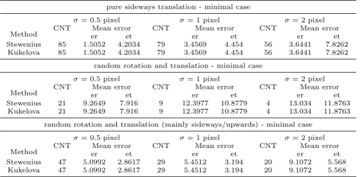
Table 1 shows the numerical results of the evaluation. Three different movement patterns were evaluated: pure sideways translation, random rotation and translation and random rotation and predominantly sideways/upwards translation. Each estimation for the different patterns and noise levels is repeated a hundred times with random movements. TheCNT-value in Table 1 indicates the number of frames where a estimation within a specified error interval is possible. Here all solutions with an translational error
less than 10◦ and all rotations with an error below 2◦are counted. These values give an indication for the percentage of acceptable solutions for hundred runs. Each experiment was realised with three levels of Gaussian noise with a standard deviationσ= (0.5,1,2) pixels.
Table 1: Comparison of mean errors for motion estimation for different movement patterns
pure sideways translation - minimal case
Method
σ= 0.5 pixel σ= 1 pixel σ= 2 pixel CNT Mean error CNT Mean error CNT Mean error
er et er et er et
Stewenius 85 1.5052 4.2034 79 3.4569 4.454 56 3.6441 7.8262 Kukelova 85 1.5052 4.2034 79 3.4569 4.454 56 3.6441 7.8262
random rotation and translation - minimal case
Method
σ= 0.5 pixel σ= 1 pixel σ= 2 pixel CNT Mean error CNT Mean error CNT Mean error
er et er et er et
Stewenius 21 9.2649 7.916 9 12.3977 10.8779 4 13.034 11.8763 Kukelova 21 9.2649 7.916 9 12.3977 10.8779 4 13.034 11.8763
random rotation and translation (mainly sideways/upwards) - minimal case
Method
σ= 0.5 pixel σ= 1 pixel σ= 2 pixel CNT Mean error CNT Mean error CNT Mean error
er et er et er et
Stewenius 47 5.0992 2.8617 29 5.4512 3.194 20 9.1072 5.568 Kukelova 47 5.0992 2.8617 29 5.4512 3.194 20 9.1072 5.568
The experiments from the original publications such as Nist´er (2004), indicate, in general, better results than see here, because only optimal geometrical configurations are allowed for the data generation (e.g. relatively wide baseline, constrained distances between object and camera, etc.). Due to the fact that this work is intended for a practical computer vision application, in this evaluation non-cooperative configurations are also allowed. There is no difference between the results of the two different methods evaluated.
A pure sideways translation leads to the best results in terms of number of acceptable solutions. The random movement pattern suffers from stereo pairs with a major forward movement, leading to ill-posed data for the estimation of the essential matrix. Based on the assumption that it is necessary to guarantee a major translational movement in x-or y-direction (wide baseline) a third motion pattern was tested which contains mainly sideways/upwards elements in the translation vector. The results clearly indicate that without an additional scheme which guarantees the usage of stereo pairs, with a relatively wide baseline, the overall accuracy (for both translational and rotational movement) is not satisfying for the intended application of 3D scene reconstruction.
5.2. Absolute pose estimation from 3D/2D correspondences
As already mentioned the usage of 3D/2D correspondences assumes the existence of a previously generated 3D scene model. For the experimental evaluation of the EPn P-approach a virtual 3D scene model is generated and projected into the image frame of a moving camera (robot) to produce the corresponding 2D feature points.
The evaluation of the accuracy of the algorithm can be realised by using the error between the given real image coordinates Ix
i and those obtained from reproject the given 3D
coordinates of the feature points in terms of WCSWX
i and the estimated rotation Re
and translationte:
I
f
xei =P
W
e Xi withP=K
Re t e
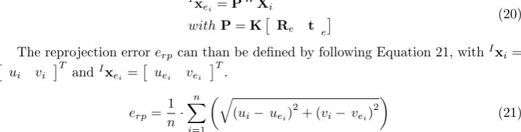
(20)
The reprojection errorerp can than be defined by following Equation 21, withIxi=
ui vi T
andIx ei=
uei vei T
.
erp=
1
n· n
X
i=1
q
(ui−uei)
2
+ (vi− vei)
2
(21)
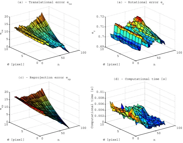
Figure 5 summarises the results for translational error (Figure 5-(a)), rotational error (Figure 5-(b)), reprojection error (Figure 5-(c)) and computational time (Figure 5-(d)) with different motion patterns, while the standard deviation of the measurement noise and the number of available correspondences is varied. Each test was repeated with 100 different configurations to show computational stability. Due to the fact that the absolute scale of the translation can be recovered by the EPnP-algorithm, the definition of the translation error as shown in Equation 17 is neglected here and the following alternative is used:
ete=kte−tk (22)
Figure 5 gives information about the general behaviour of the algorithm for different levels of noise and different number of given 3D/2D-correspondences.
It can be seen that the usage of more than 40 point correspondences leads to adequate results in terms of accuracy. It can be generally stated that the absolute pose estimation gives more accurate results than the suggested relative pose estimation techniques.
6. Conclusion and future work
The usage of both relative or absolute pose estimation techniques alone in the context of camera egomotion estimation does not guarantee reliable results. In particular, the different performances, for different motion patterns is a major problem. In this context the usage of automatic keyframe selection is necessary. In most cases a combination of an initial model generation, based on relative pose estimation and a subsequent procedure for solving the PnP-problem gives an adequate performance.
A way forward is to invoke multi-sensor data fusion (MSDF) methodologies. In this context, the combination of visual and inertial modalities although a challenging task has the potential of solving the problem of ill-posed data. In Aufderheide and Krybus (2010), an approach for camera egomotion estimation, based on visual and inertial mea-surements, where a inertial measurement unit with 9 degrees of freedoms (DoF) was used, in conjunction with an extended Kalman filtering scheme was presented. Also the combination with other sensors, besides intertial, such as radar (Silva Ruiz et al. (2011)) is a promising avenue for future research.
0 50 100 0 5 10 0 5 10 15 20 n (c) − Reprojection error e
rp
σ [pixel] erp 0 50 100 0 5 100 5 10 15 20 n (a) − Translational error e
te
σ [pixel] ete 0 50 100 0 5 10 0.69 0.7 0.71 0.72 n (a) − Rotational error e
r
σ [pixel] er 0 50 100 0 5 10 0 0.002 0.004 0.006 0.008 0.01 n (d) − Computational time [s]
σ [pixel]
Computational time [s]
Figure 5: Performance evaluation of the EPnP-algorithm for different levels of noise and number of
given correspondences: (a) - Translational errorete, (b)- Rotational erroreR, (c) - Reprojection error
erp, (d) - Computational costs
References
Aufderheide, D., Krybus, W., sept. 2010. Towards real-time camera egomotion estimation and three-dimensional scene acquisition from monocular image streams. In: 2010 International Conference on Indoor Positioning and Indoor Navigation (IPIN),. IEEE, pp. 1 –10.
Aufderheide, D., Steffens, M., Kieneke, S., Krybus, W., Kohring, C., Morton, D., 2009. Detection of salient regions for stereo matching by a probabilistic scene analysis. In: Proceedings of the 9th Conference on Optical 3-D Measurement Techniques. Wien, pp. 328–331.
Bay, H., Ess, A., Tuytelaars, T., Gool, L. V., 2008. Speeded-Up Robust Features (SURF). Computer Vision and Image Understanding 110 (3).
Br¨uckner, M., Bajramovic, F., Denzler, J., 2008. Experimental Evaluation of Relative Pose Estimation
Algorithms. In: VISAPP 2008: Proceedings of the 3rd International Conference on Computer Vision Theory and Applications. Vol. 2. pp. 431–438.
Bujnak, M., Kukelova, Z., Pajdla, T., 2008. A general solution to the P4P problem for camera with unknown focal length. IEEE Conference on Computer Vision and Pattern Recognition (2008), 1–8.
URLhttp://ieeexplore.ieee.org/lpdocs/epic03/wrapper.htm?arnumber=4587793
Davison, A., 2003. Real-time simultaneous localisation and mapping with a single camera. IEEE. Davison, A., Reid, I., Molton, N., Stasse, O., 2007. MonoSLAM: real-time single camera SLAM. IEEE
transactions on pattern analysis and machine intelligence 29 (6), 1052–67.
Gao, X.-S., Hou, X.-R., Tang, J., Cheng, H.-F., 2003. Complete Solution Classification for the Perspective-Three-Point Problem. IEEE Transactions on Pattern Analysis and Machine Intelligence 25 (8), 930–943.
URLhttp://ieeexplore.ieee.org/lpdocs/epic03/wrapper.htm?arnumber=1217599
Grunert, J. A., 1841. Das Pothenotische Problem in erweiterter Gestalt nebst Ueber seine Anwendungen
in der Geod¨asie. Grunerts Archiv f¨ur Mathematik und Physik Band 1, 238–248.
Harris, C., Stephens, M., 1988. A combined corner and edge detection. In: Proceedings of The Fourth Alvey Vision Conference. pp. 147–151.
Hartley, R., Zisserman, A., 2004. Multiple View Geometry in Computer Vision. Cambridge University Press.
Jiang, B., You, S., Neumann, U., 2000 Abstract Camera Tracking for Augmented Reality Media. Josephson, K., Byr, M., 2009. Pose Estimation with Radial Distortion and Unknown Focal Length.
Camera, 2419–2426.
URLhttp://ieeexplore.ieee.org/lpdocs/epic03/wrapper.htm?arnumber=5206756
Kruppa, E., 1913. Zur Ermittlung eines Objektes aus zwei Perspektiven mit innerer Orientierung. Kaiser licher Akademie der Wissenschaften Wien Kl Abt 122 (122), 1939–1948.
Kukelova, Z., Bujnak, M., Pajdla, T., 2008. Polynomial eigenvalue solutions to the 5-pt and 6-pt relative pose problems. BMVC.
Lepetit, V., Moreno-Noguer, F., Fua, P., 2008. EPnP: An Accurate O(n) Solution to the PnP Problem. International Journal of Computer Vision 81 (2), 155–166.
URLhttp://www.springerlink.com/index/10.1007/s11263-008-0152-6
Lepetit, V., Moreno-Noguer, F., Fua, P., February 2009. Epnp: An accurate o(n) solution to the pnp problem. Int. J. Comput. Vision 81, 155–166.
Lowe, D. G., 2004. Distinctive image features from scale-invariant keypoints. International Journal of Computer Vision 60, 91–110.
Maimone, M., Cheng, Y., Matthies, L., 2007. Two years of visual odometry on the mars exploration rovers. Journal of Field Robotics, Special Issue on Space Robotics 24, 2007.
Marzan, G. T., Karara, H. M., 1975. A computer program for direct linear transformation solution of the colinearity condition, and some applications of it. American Society of Photogrammetry, pp. 420–435.
Nist´er, D., 2004. An efficient solution to the five-point relative pose problem. IEEE transactions on
pattern analysis and machine intelligence 26 (6), 756–77.
Nistr, D., Naroditsky, O., Bergen, J., 2004. Visual odometry. pp. 652–659.
Philip, J., Oct. 1996. A Non-Iterative Algorithm for Determining All Essential Matrices Corresponding to Five Point Pairs. The Photogrammetric Record 15 (88), 589–599.
Rehrl, T., Theiß ing, N., Bannat, A., Arsi, D., Wallhoff, F., Rigoll, G., Mayer, C., Radig, B., 2010. A Graphical Model for Unifying Tracking and Classification within a Multimodal Human-Robot Interaction Scenario. Knowledge-Based Systems, 17–23.
Rodehorst, V., Heinrichs, M., Hellwich, O., 2008. Evaluation of relative pose estimation methods for multi-camera setups.
Silva Ruiz, I. R., Aufderheide, D., Witkowski, U., March 2011. Radar sensor implementation into a small autonomous vehicle. In: Proceedings of the 6th International Symposium on Autonomous Minirobots for Research and Edutainment (AMiRE 2011).
Steffens, M., Aufderheide, D., Kieneke, S., Krybus, W., Kohring, C., Morton, D., 2009a. Probabilistic Scene Analysis for Robust Stereo Correspondence. In: Lecture Notes In Computer Science; Vol. 5627. Steffens, M., Kieneke, S., Aufderheide, D., Krybus, W., Kohring, C., Morton, D., 2009b. Stereo Tracking
of Faces for Driver Observation. In: Lecture Notes In Computer Science; Vol. 5575.
Stewenius, H., Engels, C., Nister, D., Jun. 2006. Recent developments on direct relative orientation. ISPRS Journal of Photogrammetry and Remote Sensing 60 (4), 284–294.
Author Biographies
Dominik Aufderheide is an active researcher in the area of multi-sensor image
processing and computer vision. Currently he is a research fellow at the Institute of Computer Science, Vision and Computational Intelligence (CV&CI), South Westphalia University of Applied Sciences, Germany where he is working towards a Ph.D. in coop-eration with the University of Bolton, UK.
Werner Krybus is professor for data systems engineering and signal processing at
ratory for Image Processing Soest within the Institute for Computer Science, Vision and Computational Intelligence. His primary research interests include embedded systems, computer vision and sensor fusion.
Gerard Edwardsis a Senior Lecturer in Electrical and Electronics Engineering at
University of Bolton, UK. His research background is theoretical semiconductor physics and solid state electronics. In recently years his primary research area has shifted to Signal Integrity and Electromagnetic Compatibility (EMC).