Computational Simulation of Hydrodynamic Convection in Rising Bubble Under Microgravity Condition

COMPUTATIONAL SIMULATION OF HYDRODYNAMIC

CONVECTION IN RISING BUBBLE UNDER

MICROGRAVITY CONDITION

B. Asadi and M.H. Saidi*

Center of Excellence in Energy Conversion, Mechanical Engineering, Sharif University of Technology P.O. Box 11155-9567, Tehran, Iran

[email protected] - [email protected]

M. Taeibi-Rahni

Department of Aerospace Engineering, Sharif University of Technology P. O. Box 11155-9567, Tehran, Iran

[email protected]

G. Ahmadi

Department of Mechanical and Aeronautical Engineering, Clarkson University P.O. Box 13699-5725, Potsdam, New York, U.S.A.

[email protected]

*Corresponding Author

(Received: September 14, 2008 – Accepted in Revised Form: February 19, 2009)

Abstract In this work, rising of a single bubble in a quiescent liquid under microgravity condition was simulated. The related unsteady incompressible full Navier-Stokes equations were solved using a conventional finite difference method with a structured staggered grid. The interface was tracked explicitly by connected marker points via hybrid front capturing and tracking method. One field approximation was used, while one set of governing equations was only solved in the entire domain and different phases treated as one fluid with variable physical properties. The interfacial effects are accounted for by adding appropriate source terms to the governing equations. The results show that the bubble moves in a straight path under microgravity condition, compared to the zigzag motion of bubbles in the presence of gravity. Also, in the absence of gravity and temperature gradients, the hydrodynamic effect can still cause the upward motion of the bubble. This phenomenon was explicitly shown in our results.

Keywords Hydrodynamic Convection, Microgravity Condition, Hybrid Front Capturing and Tracking Method, Rising Bubble

ﻩﺪﻴﻜﭼ

ﺮﺿﺎﺣﻪﻟﺎﻘﻣﺭﺩ ،

ﻲﺒﻴﮐﺮﺗﺵﻭﺭﻪﺑﻢﮐﺶﻧﺍﺮﮔﺭﺩﺏﺎﺒﺣﺖﮐﺮﺣﯼﺯﺎﺳﻪﻴﺒﺷ ﺏﺎﺒﺣﺯﺮﻣﻲﺑﺎﻳﺩﺭﻭﺪﻴﺻ

ﺖﺳﺍ ﻩﺪﺷ ﻡﺎﺠﻧﺍ

.

ﻢﮐ ﺶﻧﺍﺮﮔ ﺕﺍﺮﺛﺍﯽﻣﻮﻤﻋ ﺕﺎﻌﻟﺎﻄﻣ ﺭﺎﻨﮐ ﺭﺩ ،

ﺯﺍ ﻲﺷﺎﻧ ﺏﺎﺒﺣ ﺯﺮﻣ ﺭﺩ ﻲﺷﺮﺑ ﻱﺎﻫﻭﺮﻴﻧ ﺪﻴﻟﻮﺗ

ﺏﺎﺒﺣﻱﺎﻨﺤﻧﺍ ﺕﺍﺮﻴﻴﻐﺗ

)

ﻲﺤﻄﺳ ﺶﺸﮐ ﻱﻭﺮﻴﻧ

(

ﺖﺳﺍ ﻪﺘﻓﺮﮔ ﺭﺍﺮﻗ ﻲﺳﺭﺮﺑ ﺩﺭﻮﻣ

.

ﻫﻭﺮﻴﻧ ﺏﺎﺒﺣﺯﺮﻣ ﺭﺩﻲﺷﺮﺑ ﻱﺎ

ﺪﻨﺷﺎﺑﻲﻣﺶﻧﺍﺮﮔﺏﺎﻴﻏﺭﺩﺏﺎﺒﺣﻲﻳﺎﺠﺑﺎﺟﺮﮔﺯﺎﻏﺁ

.

ﺮﻳﻭﺎﻧﺕﻻﺩﺎﻌﻣ

-ﻭﻩﺪﺷﻞﺣﻦﻳﺮﻠﻳﻭﺍﺖﺑﺎﺛﻪﮑﺒﺷﺭﺩﺲﮐﻮﺘﺳﺍ

ﺏﺎﺒﺣﺯﺮﻣﯼﻭﺭﻁﺎﻘﻧﺎﺑﻞﺻﺎﺣﺕﺎﻋﻼﻃﺍ ﺩﻮﺷﻲﻣﻪﻟﺩﺎﺒﻣﺖﮐﺮﺣﻝﺎﺣﺭﺩ

.

ﻲﻧﺍﺪﻴﻣﮏﺗﺐﻳﺮﻘﺗﮏﻤﮐﻪﺑ ،

ﯼﺎﻫﺯﺎﻓ

ﺮﻈﻧﺭﺩﺕﻭﺎﻔﺘﻣﻲﮑﻳﺰﻴﻓﺹﺍﻮﺧﺎﺑﻝﺎﻴﺳﮏﻳﻪﺑﺎﺸﻣﺕﻭﺎﻔﺘﻣ ﻩﺪﺷﻪﺘﻓﺮﮔ

ﺖﺳﺍ

.

ﻥﺎﻴﺑﺞﻳﺎﺘﻧ ﻂﺨﻟﺍﻢﻴﻘﺘﺴﻣﺖﮐﺮﺣﺮﮔ

ﺪﺷﺎﺑﻲﻣﺖﻔﻴﻟﻱﻭﺮﻴﻧ ﻪﻄﺳﺍﻭﻪﺑﺏﺎﺒﺣ

.

ﻞﺻﺎﺣﻲﻳﺎﺤﺑﺎﺟﻪﻄﺳﺍﻭﻪﺑﺮﻔﺻ ﺶﻧﺍﺮﮔﻂﻳﺍﺮﺷﺭﺩﺖﻔﻴﻟﻱﻭﺮﻴﻧ ﻦﻳﺍ ﺯﺍ

ﺪﺷﺎﺑﻲﻣﺏﺎﺒﺣﻱﺎﻨﺤﻧﺍﺮﻴﻴﻐﺗ

.

1. INTRODUCTION

The variation of surface tension due to temperature

variable surface tension force (not surface tension coefficient) may be generated due to the presence of surface curvature gradient. The variation of surface tension force can lead to a convective motion, which is referred to as hydrodynamic convection.

The Marangoni convection is particularly important in the absence of buoyancy. It plays a crucial role in many applications, such as in crystal growth under microgravity condition, which is of interest to microelectronic industries. Understanding the thermocapillary processes, especially process of initiation of convection and when the flow become irregular, is very important for the corresponding manufacturing processes. Most earlier technological or scientific works performed under microgravity conditions were concerned with the improvement of the material processing procedures, while the fundamental fluid mechanics of the process is not fully understood. Another important application is the boiling heat transfer for enhancing the heat exchange processes under microgravity conditions. Again, the fundamentals of microgravity boiling process are not fully understood. It is, therefore, important to have a thorough understanding of the process of bubble formation and motion under low gravity conditions, where buoyant rise is negligible. Otherwise, understanding the physics of bubble motion under microgravity condition is of great interest to a number of human life support applications in space. In this work, the isothermal rising of a single bubble in a quiescent liquid under microgravity condition was computationally investigated. The path of the bubble and the corresponding hydrodynamic Marangoni convection were evaluated. Note, the bubble was limited to a two-dimensional shape, which is a severe approximation employed to allow reasonable resolution and computational requirements. However, such a formulation allows us to observe the sole effect of the bubble dynamics.

For numerical simulation of dynamics of large bubbles, capturing and tracking of the interface is the most critical component. The computational results of Tryggvason, et al [1] have shown that the most accurate method for simulation of such flows is hybrid front capturing and tracking technique. Although, the efforts to compute multiphase flows are as old as computational fluid dynamics (CFD),

solving the full Navier-Stokes equations in the presence of a deforming interface has proven to be quite challenging. Only in recent years, major progress has been achieved with the use of the hybrid front capturing and front tracking method and also level set method.

In addition to the hybrid front capturing and front tracking technique, several other techniques have been used in the past. A summary of the relevant techniques is provided here:

1. The oldest and still the most popular approach is to capture the interface directly on a regular and stationary grid. The MAC methods, in which marker particles are advected for each fluid particle, and the VOF method, where a marker function is advected, are the best known examples. In the earlier implementations of these techniques, the stress condition at the interfaces was satisfied rather crudely. However, a number of recent developments, including a technique to include surface tension [2] and to use of “level sets” [3] to mark the fluid interface has increased the accuracy of these techniques and thus their applicability. The ferrous bio-oxidation in bubble column reactors was simulated by Vossoughi, et al [4] with using CFD approach. Mirbagheri [5], Sadrnezhad [6] also examined cavitation problem (as bubble nucleation). The heterogeneous nucleation in a uniform electric field was studied by Saidi, et al [7].

2. The second class, which potentially offers the highest accuracy, uses separate boundary fitted grids for each phase. The steady rise of buoyant, deformable, and axisymmetric bubbles were simulated by Ryskin, et al [8] using this method. Using this approach, Dandy, et al [9] also examined the steady motion of deformable axisymmetric droplets. While, Kang, et al [10] extended this methodology to axisymmetric, unsteady bubble motion. The work of Ryskin, et al [8] had a major impact on subsequent research work in this area.

4. The fourth category is the front tracking method, where a separate front marks the interface, but a fixed grid which is only modified near the front, is used for the fluid within each phase. This technique has been extensively developed by Glimm [12]. As mentioned earlier, in this work we used the hybrid front capturing and front tracking method of Tryggvason, et al [1], which is a combination of front capturing and front tracking techniques. In this method, a stationary regular grid is used for the fluid flow, while the interface is tracked by a separate grid (front grid) which is embedded on the first one but moves with the interface. Note, in the hybrid front capturing and front tracking method, all phases are treated by a single set of governing equations, while in the front tracking method each phase is treated separately. This method was developed by Unverdi, et al [13]. Loth, et al [14-16] used this method to investigate shear flow modulation and bubble dispersion of a bubbly mixing layer flow. Others also used this method to examine a number of other multiphase flow problems, e.g., collision of two equal size droplets [17]. Another use of this method was the study of the breakup of accelerated droplets where both “bag” and “shear” breakup have been observed [18].

2. IMPORTANT DIMENSIONLESS NUMBERS

The rise of a bubble in a quiescent liquid and its associated convection depend on the liquid physical properties, such as density, kinematic viscosity, and surface tension. The most important physical dimensionless numbers in such a flow are: bubble Reynolds number, ReB, Bond (Eotvos) number, Eo

(Bo), Morton number, Mo, Weber number, We, and Froude number, Fr, defined, respectively, as:

, eq r T U 2 B Re ν

= (1)

, g 2 eq r 4 ) Bo ( Eo σ ρ

= (2)

, 3 3 4 g Mo σ ρ ν

= (3)

, eq r 2 T U 2 We σ ρ

= (4)

. eq r g 2 2 T U

Fr= (5)

Here, 13

eq (3₄V)

r π

= and ρ and ν are density, viscosity of the liquid, respectively. Note that, the Morton number is related to the liquid physical properties and is independent of the flow conditions. Liquids can be categorized in different groups, namely those with high Morton numbers

) 10 Mo

( > −2 , those with intermediate Morton numbers, and those with low Morton numbers

) 10 Mo

( _< −6 _{. On the other hand, the Bond number}

characterizes the bubble size, so that a functional relationship between any parameter and the Bond number describes how that parameter changes with the bubble volume. The terminal rise velocity of bubble (UT) in Definition (1) is a function of

equivalent radius, density, kinematic viscosity, gravitational acceleration and surface tension. Note, in most practical applications, interest is mainly in low Morton numbers and moderate Reynolds numbers (between 200 and 900). At lower Reynolds numbers, however, bubbles have an approximately spherical shape, and they rise in a rectilinear path. Whereas, at intermediate and high Reynolds numbers, bubbles become oblate ellipsoids and rise in an irregular (zigzagging or spiraling) fashion. The summary of observed path and transition criteria at normal gravity is listed in Table 1 [19].

3. GOVERNING EQUATIONS

various fluids can be identified by a step (Heaviside) function (H), which takes the value of one for one particular fluid and zero for the other. The interface is marked by a non-zero value of the gradient of the step function. It is most convenient to express H in terms of an integral over the product of one-dimensional δ-functions as follows:

dA ) F y y ( A ) f x x ( ) t , y , x (

H = ∫δ − δ − (6)

The density, as well as any other physical properties, can be written in terms of both the constant densities on either side of the interface and the above Heaviside function as:

)). t , y , x ( H 1 ( o ) t , y , x ( H i ) t , y , x

( =ρ +ρ −

ρ (7)

Here, ρi and ρ0 are the density at H = 1 and 0,

respectively. On the other hand, for the viscous term, the full deformation rate tensor is implemented, while the conservative form of the advection term is normally used. Thus, the linear momentum equation is written as:

). f X X ( n k ) u T u ( . g P t D ) u ( D − δ σ + ∇ + ∇ μ ∇ + ρ + ∇ − = ρ (8)

In above equation, u is the velocity vector (either the

phases), σ is the surface tension coefficient, k is the curvature, g is the gravity acceleration, and n is a

normal vector to the bubble surface. The density (ρ) and viscosity (μ) are allowed to vary, such that these equations are therefore valid for the whole flow field (both phases), and surface tension forces have been added as a delta function δ (x-xf_{), which is non-zero}

only on the bubble surface (xf_{), where X = X}f_.

The mass conservation law is written as:

. 0 u t +∇⋅ρ = ∂

ρ ∂

(9)

In this work, the flows of fluids are both assumed to be incompressible, so that the density of a fluid particle in the flow field remains constant. Thus,

, 0 t D

Dρ₌

(10) and , 0 u . =

∇ (11)

The viscosity of each fluid particle is also assumed to be constant. Thus,

. 0 t D

Dμ₌

(12)

TABLE 1. Summary of Some Previous Experimental Results about Bubble Shape under Normal Gravity [19].

Observed Shapes and Onset of Shape Instability

Spherical Ellipsoidal Unstable

mm 42 . 0

r_eq< req<1.00mm req >1.00mm

Aybers, et al (1969)

7 . 3 We> Haberman, et al (1954) Re<400 400<Re<5000

Miksis, et al (1981) We>3.23

Contaminated Liquids Re>200

Ryskin, et al (1984)

Pure Liquids We>3−4

2 . 4 We> Duineveld (1994,1995) mm 34 . 1 r_eq >

4. NUMERICAL METHODOLOGY

In this work, the unsteady Navier-Stokes equations are solved using the finite difference method with a staggered fixed structured grid, while the interface (front) is tracked explicitly by connected marker points. The interfacial source term (surface tension effect) is computed at the front grid points and is interpolated on the fixed grid. The advection of fluid properties, such as density, is accounted for by following the motion of the front. Figure 1 shows the fixed Eulerian and the moving Lagrangian grids used. The basic idea behind the original front tracking method, illustrated in Figure 1, is fairly simple. Two grids are used. One is a standard, stationary finite difference mesh. The other is a discretized interface mesh used to explicitly track the interface. It is represented by non-stationary, Lagrangian computational points connected to form a one-dimensional line. Once the Lagrangian points are defined one must decide on a method of structuring and organizing these points. Since the interface moves and deforms during the computation, interface elements must occasionally be added or deleted to maintain regularity and stability.

For solving the governing equations, the following points have to be accounted for:

• The density and the viscosity changes due to the phase transport.

• The surface tension effect is only at the front.

• Accurate evaluation of velocity and the pressure fields at each time step.

• Accurate evaluation of motion of the interface itself.

The procedure used for evaluation of the density and viscosity transport and the surface tension term is the key element in the numerical approach. In volume of fluid (VOF) approach, an indicator function is used to identify different phases of the flow. In the hybrid front capturing and front tracking approach, however, the interface is explicitly marked and tracked. Knowing the location of the front, the values of the fluid property at different flow locations are easily specified. However, identification of the moving front is associated with the following

difficulties:

• How to best identify the front?

• How the data are transported between the fixed and the moving grids?

• How the front moves with time?

• How to satisfy the conservation laws as the front shape changes during its motion?

In the present approach, as the front shape changes, some grid points are added or subtracted to maintain proper grid for the front. Figure 2 shows a typical restructuring of the front grid. In the hybrid front capturing and front tracking approach, when data is transferred between the two grids, it is very important that the conservation laws are satisfied. To advect the discontinuous density and viscosity fields, and to compute surface tension forces, the bubble surface is represented by separate computational elements, referred to as the front. The front grid is of one lower dimension than the stationary fluid grid and is advected by the fluid velocity which is interpolated from the fluid grid. To inject surface tension forces onto the fixed fluid grid a technique that is usually called the Immersed Boundary Method and was introduced by Peskin [20] is used. In this Approach, the infinitely thin interface is approximated by a smooth distribution function that is used to distribute the surface forces over the grid points close to the surface in such a way that the total forces are conserved. Therefore, the front is given a finite thickness of about three to four grid spacings and there is no numerical diffusion of this front since the thickness remains constant for all time. To generate the density and viscosity fields from the front, a technique introduced by Unverdi et al. is used which is based on distributing the jump in these quantities onto the fixed grid by Peskin’s technique and then solving a laplace’s equation for the field variable itself. For code verification purposes, the incompressible lid-driven cavity flow was simulated. Figure 3 shows the X-velocity component profile along the vertical centerline and the Y-velocity component profile along the horizontal for Re = 100, which in compared with the results of Ghia, et al [22], showing relatively good agreements.

results are summarized in Figure 4. It is seen that, for the fist course grid, the shape of the bubble is distorted, but for the last two refined grids, the front shape are roughly the same. Thus, the 146 × 98 grid was chosen for the sake of economy of the computations.

Figure 1. Eulerian and lagrangian grids in hybrid front

capturing and front tracking technique.

Figure 2. Restructuring of a lagrangian grid.

Figure 3. X-and Y-velocity components profiles at the

centerline of the cavity.

5. RESULTS AND DISCUSSIONS

In this work, rising of a single bubble in a quiescent liquid under microgravity condition was computationally simulated. In addition to general studies of microgravity effects, the initiation of hydrodynamic convection solely due to the variations of interface curvature (surface tension force) and thus generation of shearing forces at the interfaces was also studied. The results show that the bubble moves in a straight path under microgravity condition, compared to the zigzag motion of bubbles in the presence of gravity. The related unsteady incompressible full Navier-Stokes equations were solved using a conventional finite difference method with a structured staggered grid. The interface was tracked explicitly by connected marker points via hybrid front capturing and tracking method.

Different cases studied are listed in Table 2. The selected simulation conditions are such that the bubble motion is under low or zero gravity. Different cases have been introduced in order to study both the buoyancy and hydrodynamic convection effects. According to Table 1, the bubble shape varies from spherical to ellipsoidal (or equivalent shape in 2 dimension) for different Reynolds and Bond numbers. Also, depending on these shapes, the bubble follows a straight line or zigzag curve while moving upward.

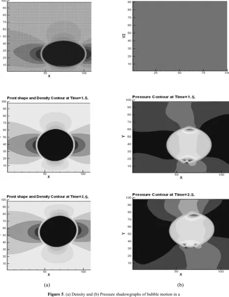
The evolutions of the pressure and density fields are shown in Figure 5. The unsteady motion of the bubble is clearly shown in this figure. Figure 6 shows the bubble shape evolution from circular at initial stage to elliptical at later times, while following a straight path. Note that in cases 1,

and 3, in the absence of gravity, the motion is only due to curvature induced lift force given as,

Lift = σknδ (X-Xf_{) (13)}

This lift force is due to surface tension coefficient and interfacial curvature. However, for initial cylindrical bubble, the value of this force is zero and thus its onset is due to initial disturbance. It should be noted that a similar phenomenon entitled “parasitic currents” has been reported specially for gas-liquid interfaces. Parasitic currents are unphysical currents generated in using implementations of the continuum surface force (CSF) technique to model surface tension forces in multi-phase computational fluid dynamics problems. However this phenomenon has a limited magnitude regarding to the fluids properties [23]. Also in our computational methodology CFS scheme has not been used. Then it seems some parts of this hydrodynamic convection can exist physically. Equation 13 shows that changes in curvature or in surface tension coefficient can initiate bubble motion even in the absence of gravity. Here, the surface tension coefficient is constant (since no temperature gradient). Thus, the only driving force for the bubble motion is the variation in the shape of the interface and initial disturbance. Figure 6 shows the evolution of the shape of the bubble with time. The results for case 2 are shown in Figure 7. As shown in this figure, when gravity is low, the buoyancy and the hydrodynamic forces tend to move the bubble. The resulting lift force is given as,

Lift = ρg + σknδ (X-Xf_{). (14)}

As expected from this figure, the bubble movement is faster here, compared to case 1.

TABLE 2. Different Test Cases Considered in This Study.

Froude Number (Fr) Weber Number (We) Morton Number (Mo) Bond Number (Eo) Reynolds Number (ReB)

Gravity (m/s2₎

Surface Tension (N/m) Case No.

∞

7.5 × 10-8

(a) (b)

Figure 5. (a) Density and (b) Pressure shadowgraphs of bubble motion in a

quiescent liquid under zero gravity condition (case 3).

S. S.

S.

S.

Figure 8 shows the results related to case 3, where surface tension coefficient is higher, but still gravity is set to zero. Note from this figure that, the bubble has higher upward velocity in comparison with the results of case 1, where surface tension coefficient was lower. The driving force for the bubble motion in this case is the hydrodynamic convection effect caused by the changes in the bubble curvature. This force is larger than the

driving force of case 1, due to higher surface tension coefficient.

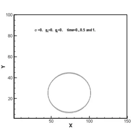
Figure 9 shows the results of case 4, where both surface tension and gravity are zero. According to Equation 14, the lift force is zero and thus there is no bubble motion with time, figure which is what has been obtained here.

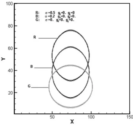
In Figure 10, cases 1, 3 and 4 are compared for t = 1 s. Note, in the absence of gravity, the higher

Figure 6. Bubble evolution (case 1).

Figure 7. Bubble evolution (case 2).

Figure 8. Bubble evolution (case 3).

the surface tension coefficient is, the higher is the upward lift force that leads to a higher bubble velocity. Also, as shown in this figure, higher surface tension coefficient causes higher upward motion of the bubble.

The results of case 1 at longer times are shown in Figure 11. The important point in this figure is that, the bubble has downward motion at t = 2 s. Here, the change in the direction of motion is due to the change in the sign of the lift force caused by changes in the bubble curvature (hydrodynamic convection effect).

6. CONCLUSIONS

In this work, large bubble motion in a quiescent liquid is computationally simulated by hybrid front capturing and front tracking method. The main conclusions are as follows:

• for all cases studied here (for the values of the dimensionless numbers studied), bubble moves in straight path, which is in contrast with the bubble motion under normal gravity condition, and

• at microgravity conditions, the driving force for the bubble motion is the variation in the bubble surface curvature. Both the buoyancy and hydrodynamic convection effects create positive lift and thus tend to move the bubble upward. However, this trend continues up to the point where the lift force changes in direction and thus the bubble moves downward.

7. NOMENCLATURES

V Bubble Volume

g Gravitational Acceleration eq

r Equivalent Radius

T

U Terminal Velocity

u Velocity Vector Field

σ Surface Tension Coefficient

n Normal Unit Vector at Interface

k Interfacial Curvature

P Pressure

ν Kinematic Viscossity Coefficint

δ Dirac Delta Function

H Heaviside Function

xf_{, y}f _{Coordinates of Nodes in Moving Grid}

x, y Coordinates of Nodes in Fixed Grid A The Bubble Surface Area

Figure 10. The comparison of marangoni force (cases 1, 3 and 4)

at t = 1 s.

Figure 11. Bubble evolution (case 1) showing negative lift

8. REFERENCES

1. Unverdi, S.O. and Tryggvason, G., “Computations of Multi-Fluid Flows”, Physica, Vol. D 60, (1992), 70-83.

2. Brackbill, J.U., Kothe, D.B. and Zemach, C., “A Continuum Method for Modeling Surface Tension”, J. Comput. Phys., Vol. 100, (1992), 335-354.

3. Sussman, M., Smereka, P. and Osher, S., “A Level Set Approach for Computing Solutions to Incompressible Two-Phase Flows”, J. Comput. Phys., Vol. 114, No. 1, (1994), 146-159.

4. Vossoughi, M. and Turunen, I., “Simulation of a Bubble Column Reactor using CFD Approach”, Multiscale Approach, European Congress of Chemical Engineering, Book of Abstracts, ECCE-6, Copenhagen, Denmark, (2007), 16-21.

5. Mirbagheri, S.A., “Solution of Flow Field Equations and Verification of Cavitation Problem on Spillway of the Dam”, International Journal of Engineering, Vol.

18, No. 1, (2005), 97-114.

6. Sadrnezhad, S.A., “Numerical Solution for Gate Induced Vibration Due to under Flow Cavitation”, International Journal of Engineering, Vol. 14, No. 13, (2001),

183-194.

7. Saidi, M.H. and Moradian, A., “Availability Analysis for Heterogeneous Nucleation in a uniform Electeric Field”, International Journal of Engineering, Vol. 16,

No. 2, (2003), 205-216.

8. Ryskin, G. and Leal, L.G., “Numerical Solution of Free-Boundary Problems in Fluid Mechanics, Part 2. Buoyancy-Driven Motion of a Gas Bubble through a Quiescent Liquid”, J. Fluid Mech., Vol. 148, (1984a),

19-35.

9. Dandy, D.S. and Leal G.L., “Buoyancy-Driven Motion of a Deformable Drop Through a Quiescent Liquid at Intermediate Reynolds Numbers”, J. Fluid Mech., Vol.

208, (1989), 161-192.

10. Kang, I.S. and Leal, L.G., “Numerical Solution of Axsymmetric, Unsteady Free-Boundary Problems at Finite Reynolds Number. I. Finite-Difference Scheme and its Applications to the Deformation of a Bubble in a Uniaxial Straining Flow”, Phys. Fluids, Vol. 30, No. 7,

(1987), 1929-1940.

11. Oran, E.S. and Boris J.P., “Numerical Simulation of Reactive Flows”, Elsevier, 1st _{Edition, New York,} U.S.A., (1987).

12. Glimm, J., “Nonlinear and Stochastic Phenomena: The Grand Challenge for Partial Differential Equations”,

SIAM Review, Vol. 33, (1991), 625-643.

13. Unverdi, S.O. and Tryggvason, G., “A Front-Tracking Method for Viscous, Incompressible Multi-Fluid Flows”, J. of Comput. Phys., Vol. 100, (1992), 25-37.

14. Loth, E., Taebi-Rahni, M. and Tryggvason, G., “Deformable Bubbles in a Free Shear Layer”, Int. J. Multiphase Flow, Vol. 23, No. 5, (1997), 977-1001. 15. Loth, E. and Taebi-Rahni, M., “Forces on a Large

Cylindrical Bubble in an Unsteady Rotational Flow”,

AICHE Journal, Vol. 42, No. 3, (1996), 638-648.

16. Loth, E., Taebi-Rahni, M. and Tryggvason, G., “Flow Modulation of a Planar Free Shear Layer with Large Bubbles-Direct Numerical Simulations”, Int. J. Multiphase Flow, Vol. 20, No. 6, (1994), 1109-1128.

17. Nobari, M.R., Jan, Y.J. and Tryggvason, G., “Head-on Collision of Drops”, Phys. Fluids, Vol. 8, (1996),

29-42.

18. Han, J., “Numerical Studies of Drop Motion in Axisymmetric Geometry”, PhD. Dissertation, Mech. Eng. Department, the University of Michigan, Ann Arbor, MI, U.S.A., (1998).

19. Vries, A.W., “Path and Wake of a Rising Bubble”, PhD Dissertation, Mech. Eng. Department, Twent University, Netherlands, (2001).

20. Peskin, C.S. and Fauci, L.J., “A Computational Model of Aquatic Animal locomotion”, J. Computational Physics, Vol. 77, (1988), 85.

21. Esmaeeli, A. and Tryggvason, G., “Direct Numerical Simulation of Bubbly Flows”, J.Fluid Mech., Vol. 37,

(2001), 313-345.

22. Ghia, U., Ghia, K.N. and Shin, C.T., “High Re-Solutions for Incompressible Flow Using the Navier-Stokes Equations and a Multigrid Method”, J. Comp. Phy.,

Vol. 48, (1982), 387-411.

23. Harvie, D.J., Davidson, M.R. and Rudman, M., “An Analysis of Parasitic Current Generation in Volume of Fuid Simulations”, J. Anziam, Vol. 46, (2005),