Please cite this article as: H. P. Patra, K. Rajnish, A New Empirical Model to Increase the Accuracy of Software Cost Estimation, International Journal of Engineering (IJE), TRANSACTIONS A: Basics Vol. 30, No. 10, (October 2017) 1487-1493
International Journal of Engineering
J o u r n a l H o m e p a g e : w w w . i j e . i rA New Empirical Model to Increase the Accuracy of Software Cost Estimation
H. P. Patra*, K. Rajnish
Department of Computer Science, BIT, Mesra, Ranchi, India
P A P E R I N F O
Paper history: Received 06 March 2017
Received in revised form 25 May 2017 Accepted 07 July 2017
Keywords: Lines of code
Software cost estimation Magnitude of Relative Error Mean Magnitude of Relative Error Pharma Research and Early Development
A B S T R A C T
We can say a software project is successful when it is delivered on time, within the budget and maintaining the required quality. However, nowadays software cost estimation is a critical issue for the advance software industry. As the modern software’s behaves dynamically so estimation of the effort and cost is significantly difficult. Since last 30 years, more than 20 models are already developed to estimate the effort and cost for the betterment of software industry. Nevertheless, these algorithms cannot satisfy the modern software industry due to the dynamic behavior of the software for all kind of environments. On this study, an empirical interpolation model is developed to estimate the effort of the software projects. This model compares with the COCOMO based equations and predicts its result analyzing individually taking different cost factors. The equation consists one independent variable (KLOC) and two constants a, b which are chosen empirically taking different NASA projects historical data and the results viewed in this model are compared with COCOMO model with different values of scale factor. In this paper the author analyze more than 250 projects collected from PROMISE repository. The effort variance is very low and the proposed model has the lowest Mean Magnitude of Relative Error (MMRE) and RMSSE.
doi: 10.5829/ije.2017.30.10a.09
1. INTRODUCTION1
This paper focused to satisfy the need of today’s software industry by estimating the cost and effort and challenging the various issues and variations occurred in software size. Accuracy and timely estimation of software efforts is one of the most critical activities to manage a software project [1, 2]. As both over estimate and under estimate of software is very harmful for modern software industry, this paper gives emphasis to predict the effort accurately and reliably. If the estimation is low then the software development team will be under pressure to finish the product and if the estimation is high then the most of the resources will be commuted to the projects [3, 4]. It is very critical to implement novel methods to improve the accuracy of a software projects. So now a days, many models are used to estimate the efforts. This model proposed an extensive COCOMO [5-7] model by changing the scale factors and constant values a, b to measure the software
*Corresponding Author’s Email: [email protected] (H. P. Patra)
effort. This paper structured as follows: Section 2 describes the overview of existing techniques, Section 3 describes a frame work to estimate the efforts as comparing with COCOMO model, and Section 4 relates the conclusion and future work.
2. OVERVIEW OF VARIOUS MODELS USED FOR SOFTWARE ESTIMATION
Since 1990 more than 20 different models are used to estimate the cost, effort, duration and productivity of the software [5, 8]. Standard models which are used to estimate the software efforts and costs are:
1. COCOMO 2. Halstead 3. Walston-Felix 4. Bailey-Basil 5. Doty (for KLOC >9) 6. SEL
2. 1. COCOMO Basic Model This model was proposed by Boehm [9] and divided by three sub
models i.e. Basic, Intermediate and detailed model [10,11] For different type of software’s basic model describes as follows (Table 1).
2. 2. COCOMO Intermediate Model
Organic Effort (E)= 3.2×(KLOC)1.05×EAF (1)
Semi Detached Effort (E) = 3.0× (KLOC)1.12×EAF (2)
Embedded Effort (E) = 2.8× (KLOC)1.2×EAF (3)
2. 3. COCOMO II Model This model formulate like:
Effort (E) =2.9 × (KLOC)1.1 (4)
2. 4. SEL Model Software engineering laboratory developed a model to estimate the software effort defined as follows.
Effort(E) = 1.4× (KLOC)0.93 (5)
Duration (D) = 4.6 × (KLOC)0.26 (6)
2. 5. Walston-Felix Model Walston and felix developed a model to estimate the efforts taking 60 IBM projects and analyzing relationship between derived lines of codes, constitutes participation, customer oriented changes and new lines of code [11].
Effort (E) = 5.2 × KLOC0.91 (7)
Duration (D) =4.1×KLOC0.36 (8)
2. 6. Bailey-Basil Model Bailey and Basil formulate a relation to estimate the efforts [12].
Effort (E) =5.5 × KLOC 16 . 1
(9)
2. 7. Halstead Models Halstead formulate a relation to estimate as [13]:
Effort (E) =0.7 × (KLOC)1.5 (10)
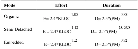
TABLE 1. Basic COCOMO Effort and Duration
Mode Effort Duration
Organic E= 2.4*KLOC1.05 D= 2.5*(PM)0.38
Semi Detached E = 2.4*KLOC1.12 D= 2.5*(PM)0.35
Embedded E= 2.4*KLOC1.2 D= 2.5*(PM)0.32
2. 8. Doty Model (KLOC>9)
Effort (E) =5.288 × (KLOC)1.047 (11)
3. PROPOSED MODEL AND METHODOLOGY
Till now, none of the existing models can measure software efforts accurately in the modern software industry for all kind of software’s. In this paper, we analyze a new empirical model for effort estimation. The cost drivers vary from project to project, so we take different scale factor values and categories the cost drivers into project, product, personal and computer.
3. 1. Data Collection For this paper, data are collected from 60 NASA projects from different containers, 93 NASA projects from common NASA2 and 63 NASA projects from promise repository. These data sets are real project data sets and may be used for practical proposes and can be viewed from “The Promise Repository of Empirical Software Engineering Data”. http://openscience.us/repo. North Carolina State University, Department of Computer Science.
3. 2. Description About Proposed Model This model is based on empirical analysis of 216 NASA Projects of different repository and it includes the scale factors like personnel, complexity, environment, risks and constraints. It predicts effort, cost estimates and reliability using the statistical approaches like y =a × (KLOC)b+ d to evaluate the cost, effort and duration empirically analyzing 216 real projects data of NASA. In this model, we use a regression formula, with the parameters ‘a’ and ‘b’ which are derived from project dataset using deterministic and heuristic methods and optimizing the global solution. By the regression analysis, we express the relationship between two variables and to estimate the dependent variable (i.e. Effort) based on independent variable (i.e. LOC) using simulated annealing algorithm [14].
F (x, y) = x2 + y2 + 5xy – 4 (12)
To get a better sense of the behavior of Equation (12), Figure 1 shows a plot of this equation.
Let suppose that the goal is to find the values of x and y that minimize f(x, y). Clearly, the solution is any point (x, y) that lies on the circle that intersects f(x, y) with the plane z = 0. We normally use simulated annealing when the solution has many variables, and finding or visualizing the solutions in these cases is much more difficult than interpreting the 3-D plot of Figure 1 [14, 16, 17].
3. 3. Proposed Algorithm Description 1. Start
2. Read the project KLOC and actual effort as E 3. Follow the equation E= n× a× (KLOC)b where a, b are constants and n is the no. of projects.
4. Σ log (KLOC) + Σ log E= n A+ B Σ log (KLOC) 5. Σ log (KLOC) × Σ log E = A Σ log (KLOC) + B (Σ (Log (KLOC)))2 Where A=log (a) and B = b+1. 6. Use the steps 4 and 5 to estimate the parameter Value of a and b by the method of statistical techniques using the data of real projects empirically 7. End.
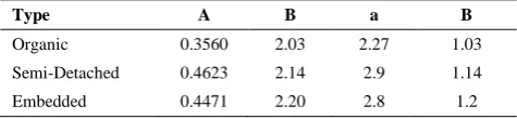
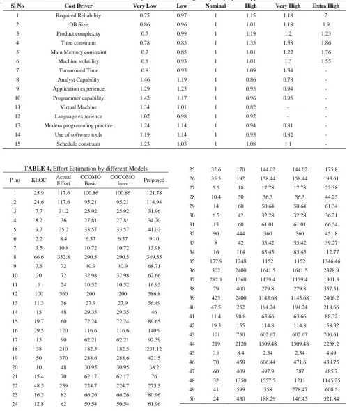
3. 4. Evolution of Proposed Algorithm Here, the authors make a convenient way to estimate the effort and the new cost driver values are taken empirically as shown in Table 3. The proposed approach provides more accurate estimation with the comparison of COCOMO model. Researchers may redefine the value of cost drivers further for better result. Individually analyzing organic, semi detached and embedded projects empirically we got the parameter value a, b as shown in Table 2.
The formula used to calculate the effort is:
Effort (E) =a ×(KLOC)b× 15 1
i NEAF+(
15 1
i NEAF+
15 1 i CEAF)
(13)
Figure 1. Example of a simulation
TABLE 2. (Predicted parameters for proposed model)
Type A B a B
Organic 0.3560 2.03 2.27 1.03
Semi-Detached 0.4623 2.14 2.9 1.14
Embedded 0.4471 2.20 2.8 1.2
where, NEAF is the new effort adjustment factors, which are new cost drivers calculated by the author in this paper empirically. CEAF are the COCOMO cost drivers, which are the COCOMO effort adjustment factors.
Effort Variance = (actual value – estimated value)/actual value.
The two main activities to calculate the effort and duration to estimate the cost of the software .This estimated effort will be converted to a dollar cost by calculating an average salary per unit time of the staff involved and multiplying this by the estimated effort required. Thus, cost of project is $ (Effort * Monthly Wages) * Total months. Table 3 describes the new effort multipliers calculated by the author to estimate the effort. Practically, it is found that the today’s software is very complex. That is why it is need of change in the cost driver value for better result and for further research the value of cost drivers may be changed for better performance.
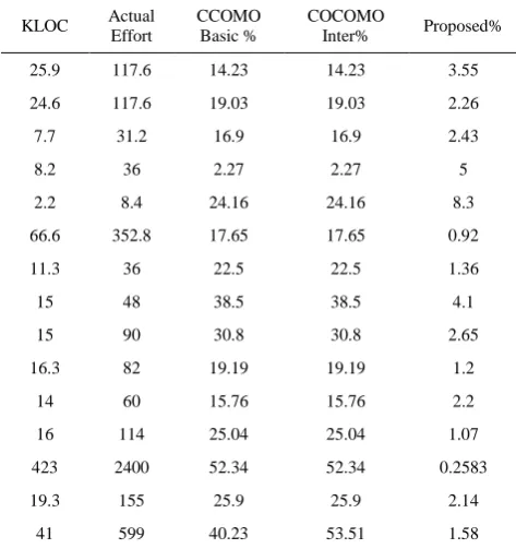
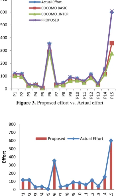
3. 5. Performance of the Proposed Model Table 4 Shows the result of effort estimation by the proposed model as comparison to COCOMO model and Table 5 shows the effort variance of different model in accordance with the data of 15 given projects and measure the performance to validate the outcome. The Performance Graph COCOMO Vs Proposed Model is shown in Figure 2, the graph of proposed model effort vs. Actual effort is shown in Figure 3 and Effort Estimation Graph of different models is shown in Figure 4.
3. 6. Evaluation Criteria and Error Analysis There are so many statistical approaches which are used to estimate the accuracy of the software effort. We are using methods like MRE, MMRE, RMSE, and Prediction [18]. Boehm [9] suggested a formula to find out the error percentage as shown below:
Error%= Actual Effort
Effort Actual Effort edicted
_
_ _
Pr
(14)
MRE (Magnitude of relative error): We can calculate the degree of estimation error for individual project.
MRE= Actual Effort
Effort edicted Effort
Actual
_
| _ Pr _
|
RMSE (Root Mean Square Error): we can calculate it as the square root of the mean square error and can be
defined as: RMSE=
. 1
2 ) _ Pr _ ( 1
n
i Actual Effort edicted Effort
n (16)
TABLE 3. New effort adjustment factors assigned by the proposed approach
Sl No Cost Driver Very Low Low Nominal High Very High Extra High
1 Required Reliability 0.75 0.97 1 1.15 1.18 2
2 DB Size 0.86 0.96 1 1.01 1.18 1.9
3 Product complexity 0.7 0.99 1 1.19 1.2 1.23
4 Time constraint 0.78 0.85 1 1.35 1.38 1.86
5 Main Memory constraint 0.7 0.85 1 1.01 1.22 1.76
6 Machine volatility 0.8 0.93 1 1.01 1.3 1.55
7 Turnaround Time 0.8 0.93 1 1.09 1.34 -
8 Analyst Capability 1.46 1.19 1 0.86 0.78 -
9 Application experience 1.29 1.23 1 0.95 0.94 -
10 Programmer capability 1.42 1.17 1 0.96 0.95 -
11 Virtual Machine 1.34 1.01 1 0.82 - -
12 Language experience 1.02 0.98 1 0.92 - -
13 Modern programming practice 1.24 1.14 1 0.94 0.81 -
14 Use of software tools 1.19 1.14 1 0.93 0.82 -
15 Schedule constraint 1.23 1.03 1 1.08 1.1 -
TABLE 4. Effort Estimation by different Models
P no KLOC Actual Effort
CCOMO Basic
COCOMO
Inter Proposed
1 25.9 117.6 100.86 100.86 121.78
2 24.6 117.6 95.21 95.21 114.94
3 7.7 31.2 25.92 25.92 31.96
4 8.2 36 27.81 27.81 34.20
5 9.7 25.2 33.57 33.57 41.02
6 2.2 8.4 6.37 6.37 9.10
7 3.5 10.8 10.72 10.72 13.98
8 66.6 352.8 290.5 290.5 349.55
9 7.5 72 40.9 40.9 68.71
10 20 72 32.98 32.98 62.66
11 6 24 10.52 10.52 16.95
12 100 360 200 200 386.8
13 11.3 36 27.9 27.9 36.49
14 15 48 29.35 29.35 46
15 19.7 60 72.24 72.24 89.65
16 29.5 120 116.6 116.6 140.9
17 15 90 62.21 62.21 92.39
18 38 210 182.5 182.5 231.12
19 50 370 288.6 288.6 421.5
20 10 48 30.95 30.95 38.2
21 15.4 70 62.17 62.17 76
22 48.5 239 224.7 224.7 273.3
23 16.3 82 66.26 66.26 80.96
24 12.8 62 50.54 50.54 61.96
25 32.6 170 144.02 144.02 175.8
26 35.5 192 158.44 158.44 193.61
27 5.5 18 17.78 17.78 22.38
28 10.4 50 36.3 36.3 44.25
29 14 60 50.64 50.64 61.34
30 6.5 42 32.28 32.28 36.21
31 13 60 61.01 61.01 66.54
32 90 444 360 360 451.8
33 8 42 35.42 35.42 39.27
34 16 114 85.45 85.45 112.77
35 177.9 1248 1152 1152 1346.46
36 302 2400 1641.5 1641.5 2378.9
37 282.1 1368 1139.4 1139.4 1301.3
38 79 400 279.8 279.8 357.51
39 423 2400 1143.68 1143.68 2406.2
40 47.5 252 194.24 194.24 218.66
41 11.4 98.8 63.66 63.66 88.32
42 19.3 155 114.8 114.8 158.32
43 101 750 602.67 602.67 700.61
44 219 2120 1509.48 1509.48 2258.2
45 0.9 8.4 2.34 2.34 4.49
46 70 458 606.44 471.6 438.75
47 60 409 497.9 387 485.7
48 32 1350 1557.5 1211 1145.25
49 41 599 358 278.47 608.5
TABLE 5. Effort variance (%) by different Models (Data of 15 projects out of 93 NASA data)
KLOC Actual Effort
CCOMO Basic %
COCOMO
Inter% Proposed%
25.9 117.6 14.23 14.23 3.55
24.6 117.6 19.03 19.03 2.26
7.7 31.2 16.9 16.9 2.43
8.2 36 2.27 2.27 5
2.2 8.4 24.16 24.16 8.3
66.6 352.8 17.65 17.65 0.92
11.3 36 22.5 22.5 1.36
15 48 38.5 38.5 4.1
15 90 30.8 30.8 2.65
16.3 82 19.19 19.19 1.2
14 60 15.76 15.76 2.2
16 114 25.04 25.04 1.07
423 2400 52.34 52.34 0.2583
19.3 155 25.9 25.9 2.14
41 599 40.23 53.51 1.58
MMRE (Mean Magnitude of Relative Error): It is another way to measure the performance and it calculates the percentage of absolute values of relative errors. It is defined as:
MMRE=
n
i Actual Effort
Effort Actual effort edicted
n 1 _ .
| _ _
Pr |
1
(17)
PRED (N): This criteria is used to calculate the average percentage of estimates that were within N% of the actual values i.e. the percentage of predictions that fall within p % of the actual, denoted as PRED (p). Where k is the number of projects in which MRE is less than or equal to p, and n is the total number of projects. It is defined as PRED (p) = k / n.
For project 1 having KLOC =25.9, the actual effort is 117.6 Man-Month and calculated effort for Basic COCOMO and Intermediate COCOMO is 100.86 MM and by the proposed model is 121.78 MM. Similarly, for project 2 KLOC=24.6, the actual effort is 117.6 MM and calculated effort for Basic COCOMO and Intermediate COCOMO is 95.21 MM and by the proposed model is 114.94 MM. Now, we can calculate the % of error using the Equation (5). For project 1, the error % for Basic COCOMO and Intermediate COCOMO is (-14.23) % and error % for proposed model is (+3.55) %. Similarly, For project 2, the error % for Basic COCOMO and Intermediate COCOMO is (-19.03) % and error % for proposed model is (-2.26) %. Here, the negative % indicates the under estimation of
the project and positive % error indicates the project is over estimate. Big under estimate gives extra pressure to the developing staff and leads to add more staffs which causes the late to finish the project. According to Parkinson’s Law of “Work expands to fill the time available for its completion”, Big over estimation reduces the productivity of personnel [19]. So, during the estimation, researchers should have to give emphasis to reduce the big over or under estimation of the project.
3. 7. Comparison with COCOMO Models In software estimation, COCOMO model is a regular and standard model to estimate the effort developed by Barry Boehm. However, in the proposed model the researcher used a basic regression formula, with parameters which are derived from historical project (NASA software). Here, we are estimating the effort based on the actual project characteristic data and better result predicts as compare to MMRE and RMSE as shown in the graph. Considering the data, the researcher changed the cost driver value and the parameters [20].
3. 8. Advantages of Proposed Model It Is reusable
It calculates software development effort as a function of program size expressed in Kilo Lines of code (KLOC)
It predicts the estimated effort with more accuracy.
TABLE 6. Performance of Different Models Performance COCOMO Basic COCOMO Inter Proposed
MMRE 0.2436 0.25185 0.0249
RMSE 69.07 89.22 3.586
PRED (12%) 0.16 0.25 0.69
Figure 2. Performance Graph COCOMO Vs Proposed Model
0 50 100
4. CONCLUSION AND FUTURE WORK
This proposed model can be useful to estimate the software effort with better accuracy which is very important when software pays a lot in every industry. In this paper, the author analyzes more than 250 projects collected from PROMISE repository. The predicted result shows there is very close values between actual and estimated effort. The effort variance is very less and the proposed model has the lowest MMRE and RMSSE and prediction values of 0.0249 and 3.586 and 0.69, respectively. So, the proposed model may able to provide good estimation capabilities for today’s software industry
Figure 3. Proposed effort vs. Actual effort
Figure 4. Effort Estimation Graph of different models
5. REFERENCES
1. Seth, K. and Sharma, A., "Effort estimation techniques in component based development-a critical review proceedings of
the 3rd national conference", INDIACom-2009, New Delhi, India.
2. Shepperd, M. and Schofield, C., "Estimating software project effort using analogies", IEEE Transactions on Software
Engineering, Vol. 23, No. 11, (1997), 736-743.
3. Maxwell, K.D. and Forselius, P., "Benchmarking software development productivity", Ieee Software, Vol. 17, No. 1, (2000), 80-88.
4. Molokken, K. and Jorgensen, M., "A review of software surveys on software effort estimation", in Empirical Software Engineering. ISESE 2003. Proceedings. 2003 International Symposium on, IEEE., (2003), 223-230.
5. Boehm, B.W., "Software engineering economics, Prentice-hall Englewood Cliffs (NJ), Vol. 197, (1981).
6. Srivastava, D.K., Chauhan, D.S. and Singh, R., "Square model-a software process model for ivr software system".
7. Jorgensen, M. and Sjoberg, D.I., "The impact of customer expectation on software development effort estimates",
International Journal of Project Management, Vol. 22, No. 4,
(2004), 317-325.
8. Uysal, M., "Estimation of the effort component of the software projects using simulated annealing algorithm", New Trends in Technologies, DOI: 10.5772/7583, (2008).
9. Boehm, B.W., "Understanding and controlling software costs",
Journal of Parametrics, Vol. 8, No. 1, (1988), 32-68.
10. Attarzadeh, I. and Ow, S.H., "A novel soft computing model to increase the accuracy of software development cost estimation", in Computer and Automation Engineering (ICCAE), 2010 The 2nd International Conference on, IEEE. Vol. 3, (2010), 603-607.
11. Deshpande, M. and Bhirud, S., "Analysis of combining software estimation techniques", International Journal of Computer
Applications (0975–8887), Vol. 5, No. 3, (2010), DOI:
10.5120/901-1277.
12. Bailey, J.W. and Basili, V.R., "A meta-model for software development resource expenditures", in Proceedings of the 5th international conference on Software engineering, IEEE Press., (1981), 107-116.
13. Benediktsson, O. and Dalcher, D., "Effort estimation in incremental software development", IEE Proceedings-Software, Vol. 150, No. 6, (2003), 351-357.
14. Ledesma, S., Avina, G. and Sanchez, R., Practical considerations for simulated annealing implementation, in Simulated annealing. 2008, InTech.
15. Suri, P., Bhushan, B. and Jolly, A., "Time estimation for project management life cycle: A simulation approach", International
Journal of Computer Science and Network Security, Vol. 9,
No. 5, (2009), 211-215.
16. Ali, M., Torn, A. and Viitanen, S., A direct search simulated annealing algorithms for optimization involving continuous variables. (1997), Technical report, Turku Centre for Computer Science, Abo Akademi University, Finland.
17. Goel, T. and Stander, N., "Adaptive simulated annealing for global optimization in ls-opt", in Proceedings of the 7th European LS-DYNA Conference. California: LSTC., (2009), 1-8.
18. Pressman, R.S., "Software engineering: A practitioner's approach, Palgrave Macmillan, McGraw-Hill Education; 8 edition, ISBN-10: 0078022126, (2005).
19. Jalote, P., "An integrated approach to software engineering", Springer Science & Business Media, ISBN 978-0-387-28132-2, (2012).
0 100 200 300 400 500 600 700
P1 P2 P3 P4 P5 P6 P7 P8 P9 10P P11 P12 P13 P14 P15 Actual Effort
COCOMO BASIC COCOMO_INTER PROPOSED
0 100 200 300 400 500 600 700 800
P1 P2 P3 P4 P5 P6 P7 P8 P9 10P P11 P12 P13 P14 P15
Ef
fo
rt
A New Empirical Model to Increase the Accuracy of Software Cost
Estimation
TECHNICAL NOTE
H. P. Patra, K. Rajnish
Department of Computer Science, BIT, Mesra, Ranchi, India
P A P E R I N F O
Paper history: Received 06 March 2017
Received in revised form 25 May 2017 Accepted 07 July 2017
Keywords: Lines of code
Software cost estimation Magnitude of Relative Error Mean Magnitude of Relative Error Pharma Research and Early Development
ديكچ ه
زاین دروم تیفیک ظفح اب و هجدوب دودح رد ،عقوم هب نآ هک تسا قفوم ینامز یرازفا مرن هژورپ کی مییوگب میناوت یم ام روطنامه .تسا هتفرشیپ رازفا مرن تعنص یارب مهم هلئسم کی رازفا مرن هنیزه دروآرب هزورما ،لاح نیا اب .دوش هداد لیوحت روط هب نردم رازفا مرن هک زا .تسا لکشم رایسب شلات و اه هنیزه دروآرب نیاربانب ،دنک یم راتفر ایوپ
30 شیب ،هتشذگ لاس
زا 20 .تسا هتفای هعسوت رازفا مرن تعنص دوبهب یارب هنیزه و شلات یبایزرا یارب لدم یمن اه متیروگلا نیا ،دوجو نیا اب
یکیمانید راتفر هب هجوت اب ار نردم رازفا مرن تعنص دنناوت .دنزاس هدروآرب طیحم عون همه یارب رازفا مرن
،هعلاطم نیا رد
ینتبم تلاداعم اب لدم نیا .تسا هدمآ دوجو هب یرازفا مرن یاه هژورپ شلات دروآرب یارب یبرجت یبای نورد لدم کی رب
COCOMO
یزه فلتخم لماوع نتفرگ رظن رد اب هناگادج لیلحت و هیزجت اب ار نآ هجیتن و دوش یم هسیاقم شیپ هن
لقتسم ریغتم کی لماش ،هلداعم .دنک یم ینیب
(KLOC)
تباث ود و
a
و
b
هژورپ یلبق یاه هداد زا یبرجت روط هب هک تسا
لدم اب لدم نیا رد هدش هدهاشم جیاتن و هدش باختنا اسان فلتخم یاه
COCOMO
سایقم روتکاف فلتخم ریداقم اب
زا شیب هدنسیون ،هلاقم نیا رد .دوش یم هسیاقم 250
نزخم زا هک ار هژورپ
PROMISE
.دنک یم لیلحت ،هدش یروآ عمج
یبسن یاطخ نیگنایم نیرتمک یاراد یداهنشیپ لدم و تسا مک رایسب شلات سنایراو
(MMRE)
و
RMSSE
.تسا