A SYNCHROPHASOR
APPLICATION IN VOLTA GE
REGULATI ON
ABSTRACT
As population growth increases power demand, power industries all around the world become increasingly complex; and therefore, unpredictable. Hence, it is not surprising that undesirable events such as voltage collapse and power blackout incidents occur more frequently. However, since the healthy operation of power systems not only increases distribution efficiency but also reduces cost and allows for a safe operation, the power industry is challenged with the
development of countermeasures in order to mitigate the occurrence of these undesirable events and enable the maintenance of an acceptable level of operation at all times. Analyses of power blackout events have allowed the power industry to gain a clearer insight as to its causes which can be surmised in three points: loss of system stability, lack of situational awareness [1] and incorrect actions by network operators.
However, with the advent of synchrophasor technology, it is now possible to have real-time, time-synchronized network measurements. Furthermore, with the use of stability indices, it is possible to indicate system stability via scalar values. The combination of synchrophasor technology and stability indices eliminates, to a reasonable extent, the lack of situational awareness as it specifically enables network operators to assess system stability using reliable, real-time data.
AKNOWLEDGEMENTS
Firstly, I would like to acknowledge my supervisor; Dr. Gregory Crebbin, for his assistance in the completion of the project. He has taught me that the best way to learn is to ask a lot of questions and follow through with a significant amount of research.
Additionally, I would also like to show my appreciation to Dr. Sujeewa Hettiwatte who spared some of his time to discuss and answer a few of my question.
And to my friends who keep me motivated during the ups and downs of this project. They continue to remind me that a simple but effective method of learning is simply discussing with friends:
Nick Kilburn, 4th year Power and Industrial Computing Marc Purvis, 4th year Power and Industrial Computing
Tanvi Gupta, 4th year Renewable and Instrumentation/Control Nurazlina Mohamad Nain, Masters in Instrumentation/Control
Chapter 1:
CONTENTS
Abstract ...i
Aknowledgements ... ii
List of Figures ... v
List of Tables ... 6
Chapter 1: Introduction ... 1
Chapter 2: Project Overview ... 3
2.1 Project Stages ... 3
2.2 Synchrophasors ... 4
2.2.1 Phasor Derivation ... 6
2.3 System Stability ... 7
2.3.1 Overview ... 9
2.3.2 System Analysis ... 10
2.3.3 Types of System Stability ... 13
2.3.4 Stability Algorithms ... 19
2.4 Thevenin Equivalence Algorithm ... 24
2.5 Simulation Programs and Software ... 28
2.5.1 Matlab by MathWorks ... 28
2.5.2 PowerFactory by DIgSILENT ... 28
Chapter 3: Stability Analysis using Stability Indices ... 29
3.1 Test Networks ... 29
3.1.1 Test Power Network 1 ... 30
3.1.2 Test Power Network 2 ... 30
3.2 Test Cases ... 31
3.3 Task Implementation... 31
3.4 Results... 32
3.5 Analysis and Comparison... 37
Chapter 4: Stability Indices in Voltage Regulation ... 39
4.1 Voltage Regulation ... 39
4.1.1 Voltage Regulation Devices ... 40
4.2 Proposed Structure ... 43
4.3 Example ... 44
4.3.1 Implementation ... 44
4.3.2 Results ... 45
Chapter 5: Challenges and Recommendations... 47
5.1 Software Interconnectivity ... 47
5.2 Stability Indices ... 48
5.3 Synchrophasors ... 48
Chapter 6: Future Work... 49
Chapter 7: Conclusion ... 50
Chapter 8: Bibliography ... 51
Chapter 9: Appendix ... 54
9.1 Data For Test Power Networks ... 54
9.1.1 Test Power System Network 1 ... 54
9.1.2 Test Power System Network 2 ... 55
9.2 Stability Indices for Test Power Networks ... 56
9.2.1 Test Power System Network 1 ... 56
9.2.2 Test Power System Network 2 ... 58
9.3 Matlab Algorithms ... 60
9.3.1 Main File ... 60
9.3.2 Thevenin File ... 62
9.3.3 Stability Indices File ... 64
9.3.4 Data Acquisition File ... 67
LIST OF FIGURES
Figure 1: Project Structure indicating its 3 stages ... 3
Figure 2: Generic 2-bus system waveform highlighting time point 0.0167s ... 5
Figure 3: Generic synchrophasor control structure ... 6
Figure 4: Image depicting the ‘phase-calculation’ method of a synchrophasor ... 7
Figure 5: Image depicting a form of stability (1) ... 8
Figure 6: Image depicting a form of stability (2) ... 8
Figure 7: Image depicting a form of stability (3) ... 8
Figure 8: A simple r-l-c circuit ... 11
Figure 9: Classifications of power system stability (adapted from [5]) ... 13
Figure 10: A simple 2-bus system ... 15
Figure 11: Plot showing Vs for a system with =0.5, =0 and =1.0 ... 18
Figure 12: A simple system for thevenin calculation ... 24
Figure 13: A System complex system for thevenin calculation (adapted from the ieee’s 14 test Power system) ... 24
Figure 14: Perception of the thevenin equivalence algorithm ... 26
Figure 15: Test Power Network 1 ... 29
Figure 16: Test Power Network 2 (IEEE Adapted [18] and [19] ) ... 30
Figure 17: Stability plot derived by increasing load 2’s reactive power (10% increment of initial Load q in Per Unit) ... 33
Figure 18: Stability plot derived by increasing load 2’s active power (10% increment of initial Load P in Per Unit) ... 33
Figure 19: Voltage-Power plot showing load 2’s final Power state in Red (During 10% increment of initial Load P In Per Unit) ... 34
Figure 20: Stability plot derived by increasing load 1’s reactive power (10% increment of initial Load q in Per Unit) ... 35
Figure 21: Stability plot derived by increasing load 1’s active power (10% increment of initial Load P in Per Unit) ... 36
Figure 22: Voltage-Power plot shwoing load 1’s final state in Red (During 10% increment of initial Load P in Per Unit) ... 36
Figure 23: An Example of the effect of a shunt capacitor bank (where 0.45pu QL is required) ... 41
Figure 25: Simple 4-bus system to be used as Example (Normal Operation: T2 Tap = 3 and Load
voltage = |0.9439| at -5.8969°) ... 44
Figure 26: (PowerFactory) Transformer Tap and Load Voltage under VR+SI (Initial state as in Figure 25) ... 45
Figure 27: (PowerFactory) Transformer Tap and Load Voltage under VR+SI (Load Power = 48MWW + 18MVar) ... 46
Figure 28: Data 1 test Power Network 1 ... 54
Figure 29: Data 2 test Power Network 1 ... 54
Figure 30: Data 1 test Power Network 2 ... 55
Figure 31: Data 2 test Power Network 2 ... 55
Figure 32: Stability indices for Test Power Network 1 with varying Reactive Power (load 1) ... 56
Figure 33: Stability indices for Test Power Network 1 with varying Reactive Power (load 2) ... 56
Figure 34: Stability indices for Test Power Network 1 with varying Active Power (load 1) ... 57
Figure 35: Stability indices for Test Power Network 1 with varying Active Power (load 2) ... 57
Figure 36: Stability indices for Test Power Network 2 with varying Reactive Power (load 5 or 1) ... 58
Figure 37: Stability indices for Test Power Network 2 with varying Reactive Power (load 6 or 2) ... 58
Figure 38: Stability indices for Test Power Network 2 with varying Reactive Power (load 8 or 3) ... 58
Figure 39: Stability indices for Test Power Network 2 with varying Active Power (load 5 or 1) 58 Figure 40: Stability indices for Test Power Network 2 with varying Active Power (load 6 or 2) 59 Figure 41: Stability indices for Test Power Network 2 with varying Active Power (load 8 or 3) 59
LIST OF TABLES
Table 1: Tabulated data of some power collapse events (adapted from [2], [3] and [4]) ... 1Table 2: Some operating point properties for test power networks 1 and 2 ... 37
Table 3: Data for Example System ... 44
Table 4: (Matlab) Transformer Tap and Load Voltage under VR+SI (Initial state as in Figure 25) ... 45
Table 5: (Matlab) Transformer Tap and Load Voltage under VR+SI (Load Power = 48MWW + 18MVar) ... 46
Chapter 1:
INTRODUCTION
Over the years, power transmission and distribution networks all around the world have experienced a significant number of power blackouts incidents. A power blackout can be defined as the loss of power in the whole or significant parts of a power distribution network. A few blackout incidents are provided in Table 1.
TABLE 1: TABULATED DATA OF SOME POWER COLLAPSE EVENTS (ADAPTED FROM [2], [3] AND [4])
Voltage Collapse Incidents
Date Location Trigger Time Frame
22/09/1970 New York, USA Lightning Strike > 24 hrs
19/12/1978 France Rotor Instability: loss of synchronism > 1 hr 23/08/1987 Tokyo, Japan Voltage Instability: high power demand > 1 hr
14/08/2003 Cleveland, USA Short Circuit fault > 24 hrs
30/07/2012 India Line Overload >12 hrs
22/08/2013 Sydney, Australia Unknown > 1 hr
Based on the information provided in Table 1, it is obvious that the triggering event for voltage collapse in a power system varies: from a simple line fault to voltage instability (unacceptable bus voltages during normal and disturbance-recovery conditions) and rotor instability
(de-synchronization of the system’s synchronous machines by 180⁰ or more). However, as blackout events
have occurred since the early 20’s, the power industry’s understanding of these events is ever-growing; and recent blackout incidents have provided an even clearer picture as to the roots of this problem. The causes of power blackout can be surmised in three points: loss of system stability, lack of situational awareness [1] and incorrect actions by network operators.
The first stage is the loss of system stability. System instability can be defined as the inability of a power system (power network) to maintain an acceptable level of operation. As inferred from [5], system instability can occur during normal operation or during recovery operation subsequent to interference from a disturbance. Regardless of its form, the loss and continued deterioration of system stability is the first event in the sequence of events that leads to power blackout.
Secondly, measurement devices were not synchronized to each other. Since most electrical calculations require system parameters to be measured at the same time, the measurement of parameters such as source and load bus voltages which are separated in space would be separated in time as well; and thus, could not be used for stability assessment.
Consequently, with the loss of system stability combined with the unawareness of system state, it becomes very easy for network operators to take incorrect and delayed responses to perceived
disturbances. These responses can further deteriorate system stability leading to voltage collapse and, finally, to a power blackout.
This project proposes the use of synchronized measurements obtained from synchrophasor
Chapter 2:
PROJECT OVERVIEW
This section gives a brief overview of major concepts pertinent to this project. They include
Synchrophasors, Power System Stability, Stability Algorithms, Voltage Modeling, Voltage Regulation and Simulation Software.
2.1
PROJECT STAGES
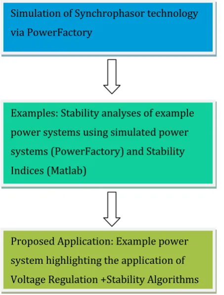
As illustrated in Figure 1, the project is divided into three (3) stages: simulation of synchrophasor technology via power system simulator (PowerFactory), verification of stability algorithms, and lastly, incorporation of a selected stability algorithm in voltage regulation.
FIGURE 1: PROJECT STRUCTURE INDICATING ITS 3 STAGES
The first stage refers to the simulation of synchrophasor data using power network simulation software, in particular, DIgSILENT’s PowerFactory. As this stage involves the simulation of selected power systems and data acquisition from these selected power systems, it is more of an underlying stage that will reoccur throughout this project. The aforementioned software will be briefly discussed in section 2.5.
Stage 2; serving as the foundation stage, is concerned with the familiarization, Matlab programming and interpretation of selected stability indices. As these indices are will be used in subsequent
Simulation of Synchrophasor technology via PowerFactory
Examples: Stability analyses of example power systems using simulated power systems (PowerFactory) and Stability Indices (Matlab)
Procedurally, the stability indices are programmed in MathWorks’ Matlab and data from 2 power systems are used as inputs. These data are derived from power system simulations conducted in PowerFactory where system measurements such as voltage phasor and load power simulate
synchrophasor measurements. The resulting array of scalar indices will be plotted in order to visually inspect the stability trend of load terminals or buses. In a sense, this task serves as the core activity for this project since adequate knowledge of the selected stability indices will be required for the
successful completion of the project.
Following the completion of stage 2 is the final stage of this project; Stage 3. In this last stage of the project, the aim is to successfully simulate incorporate stability assessment; via stability indices, into voltage regulation procedure. A method for incorporating stability indices will be proposed and presented by creating a simple voltage regulation algorithm in Matlab while using system data from PowerFactory as inputs to simulate measurements from synchrophasor technology. Thereafter, a chosen stability indices will be included in the voltage regulation algorithm in order to show, to an extent, the potential advantage that will arise from the use of synchrophasor technology and stability indices in voltage regulation.
2.2
SYNCHROPHASORS
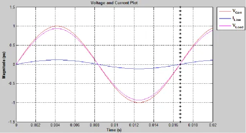
Synchrophasors or “Synchronous Phase Measurement Units” refer to the characteristics of a device to “… provide a real-time measurement of electrical quantities from across the power system” [6]. In order to gain a better understanding of the advantage synchrophasors introduce, consider, for example, the waveforms shown in Figure 2. It depicts the waveforms corresponding to generated voltage, load voltage and line current in a generic 2-bus power system where generator, transmission line and load are all connected in series. At time ’0.0167s’, highlighted in the figure, the single-phase active power of the generator and load; and , can be calculated according to Equation 1 and Equation 2 respectively. Comparison of generator and load power are required in various system analyses such as the quick determination of a system’s power transfer efficiency with respect to time. However, such analyses are only truly accurate when generator and load parameters are measured at exactly the same time (voltage and line current at time point ‘0.0167s’ in this
EQUATION 1: INSTANTANEOUS ACTIVE POWER AT GENERATOR’S BUS
EQUATION 2: INSTANTANEOUS ACTIVE POWER AT LOAD’S BUS
where:
FIGURE 2: GENERIC 2-BUS SYSTEM WAVEFORM HIGHLIGHTING TIME POINT 0.0167S
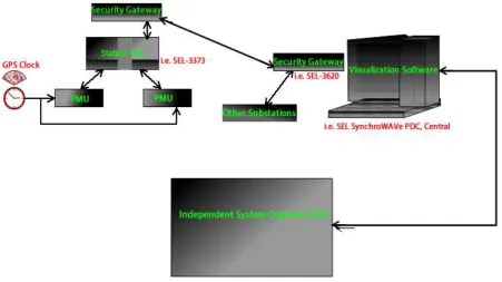
Compared to previous SCADA-only control methods, the incorporation of synchrophasors introduces the additional advantage of time-synchronized data, thus, improving data accuracy, reliability, acquisition speed as well as usefulness in stability analysis. Mainly achieved through the incorporation of GPS satellite-synchronized clocks, synchrophasor applications include voltage regulation, model verification, system stability analysis and islanding detection. Other devices in a synchrophasor structure are illustrated in Figure 3. These include Phasor Measurement Units
FIGURE 3: GENERIC SYNCHROPHASOR CONTROL STRUCTURE
2.2.1
PHASOR DERIVATION
Mathematically, an alternating-current (ac) waveform can be defined according to Equation 3. Consequently, the corresponding phasor equivalent of the ac waveform is according to Equation 4.
EQUATION 3: GENERIC AC WAVEFORM
EQUATION 4: PHASOR REPRESENTATION OF AC WAVEFORM
EQUATION 5: PHASOR REPRESENTATION OF AC WAVEFORM IN RMS
where:
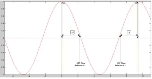
Synchrophasor calculations operate according to Equation 5, the RMS variant of Equation 4. Figure 4 graphically represents the phasor derivation process that is used in calculating synchrophasor values.
FIGURE 4: IMAGE DEPICTING THE ‘PHASE-CALCULATION’ METHOD OF A SYNCHROPHASOR
As stated in [7], UTC (Coordinated Universal Time) Time Reference 1 and UTC (Coordinated Universal Time) Time Reference 2 in Figure 4 can be perceived as time strobes or reference points. Assuming constant frequency at steady state, angle ‘+θ*’ and its corresponding cosine wave
magnitude ‘X1’ occur at UTC 1. Similarly, at the instance UTC 2 occurs, angle ‘-θ*’ is the angle difference to its closest cosine reference angle and ‘X2’ is its corresponding cosine wave magnitude. However, since power systems rarely operate at a constant frequency, the final calculation of ‘θ*’ takes into account the actual frequency at the time of measurement. Additional information such as reporting rates and performance criteria are further discussed in [7] and [8].
2.3
SYSTEM STABILITY
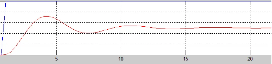
desirable operating region regardless of disturbances. This is further illustrated in Figure 5, Figure 6 and Figure 7 where bounded inputs are plotted (blue line) and compared with the resulting response of a system (red line). According to the definitions above, these system responses can be deemed as stable regardless of their transient characteristics. This is because all three figures show system responses that settle within a bounded region after experiencing a bounded change in input – an impulse input in Figure 5’s system and a step input in the systems shown in Figure 6 and Figure 7.
FIGURE 5: IMAGE DEPICTING A FORM OF STABILITY (1)
FIGURE 6: IMAGE DEPICTING A FORM OF STABILITY (2)
FIGURE 7: IMAGE DEPICTING A FORM OF STABILITY (3)
2.3.1
OVERVIEW
The stability analysis of a power system is an important task of network operators. In [5], a brief history of stability in the power industry is given. It details how the concept of power system stability was recognized as pertinent in 1920. At this time, stability issues alluded to hydroelectric generating stations transmitting power over long distances. For economic reasons, these stations operated at points close to their stability limits; hence, instability occurred frequently. Additionally, with methods such as the ‘equal-area criterion’ and ‘circle diagrams’ in use, the power system network to be
analyzed had to be kept simple. However, with the increase in interconnected independent power systems driven by economical benefit, stability problems also increased. It was only with the development of the ‘network analyzer’ (ac calculating board) in 1930 that the analysis of more complex power system networks became possible. At present, with the continuous improvement in digital computer technologies, modeling methods for significant network equipment, developments in control system theory and fast-reacting fault clearing devices, there is a clearer understanding of stability events as well as methods for mitigating and countering such events.
Traditionally, a common requirement for the stable and satisfactory operation of a power system is that all synchronous machines must be operated in synchronism. As stated in [5], this implies that the frequency of the stator’s electrical quantities; induced voltage and resulting current, must be identical to the mechanical speed of the rotor. However, instability can still occur without the loss of
2.3.2
SYSTEM ANALYSIS
Generally, almost all power system analysis can be completed either through the assumption of steady state or by considering the dynamic behavior of the power system via transient analysis. Although each analysis method holds its own advantages and disadvantages, steady-state analyses are known to be less complicated and less time consuming. On the other hand, transient analysis holds the advantage of providing detailed insight on salient characteristics as the power system undergoes a change.
2.3.2.1 STEADY STATE ANALYSIS
Defined as “A stable condition that does not change over time or in which change in one direction is continually balanced by change in another.”[10], steady state analysis is the most common method of analysis for power systems. It assumes that, at the moment in time of the analysis, the power system parameters of interest are non-changing. Consider the circuit depicted in Figure 8, where the system element subscript ‘R’, ‘C’ and ‘L’ denotes resistance, capacitance and inductance. Their corresponding impedances would be modeled as variables unchanging in time. That is, ‘ZR’ – resistive portion of overall impedance, ‘ZC’ – capacitive portion of overall impedance and ‘ZL’ – resistive portion of overall impedance, will be unchanging with respect to time. These are defined in Equation 6.
EQUATION 6: (STEADY STATE) OVERALL IMPEDANCE
EQUATION 7: (STEADY STATE) CURRENT FLOWING IN THE SERIES-CONNECTED SYSTEM
EQUATION 8: (STEADY STATE) VOLTAGE ACROSS THE CAPACITOR
where:
FIGURE 8: A SIMPLE R-L-C CIRCUIT
In terms of system stability, analysis completed via steady state method can provide useful
information on the initial and final state of the power system; thus, allow for preemptive actions in order to dampen or eliminate undesirable effects. The collection of steady state data; such as steady state voltages and currents, can be used to determine salient system characteristics required for various stability analyses. Under various conditions, recorded steady state parameters can be used in the development of stability trends and plots. Consequently, this would allow for the comparison of various system states; thereby providing sufficient information to determine whether or not corrective actions are required.
For instance, re-consider the system depicted in Figure 8. Under the assumption that the system experienced a 10% load (demanded power) increase, the current phasor flowing through the capacitive load, prior to the increase, is given by Equation 7. Similarly, the current phasor flowing, after the load increase, can also be calculated using Equation 7 while taking into account that the system load is now
. Following a similar procedure, the initial and final voltage phasor across the capacitive load can be determined according to Equation 8. By taking these values into consideration during stability analysis, a fair indication of power system’s stability can be derived. On the other hand, the intermediate behaviors of a power system and its parameters can only be
2.3.2.2 TRANSIENT ANALYSIS
As defined in [11], transient analytical method is used to describe the behavior of power system parameters during the transition between two distinct steady-state conditions. This usually implies that the analysis is carried out over a range of time, either continuously or in discrete steps.
Consequently, this also implies that parameter modeling as well as system element models would be time-based. Reconsider the R-L-C circuit introduced in Figure 8. As opposed to steady state analysis, system elements would be modeled with respect to their change in time. Hence, the voltage across the capacitor, as well the current flowing through it, would be represented according to Equation 9 and Equation 10 .
EQUATION 9: (TRANSIENT STATE) VOLTAGE ACROSS THE CAPACITOR
EQUATION 10: (TRANSIENT STATE) CURRENT FLOWING THROUCH THE CAPACITOR
where:
2.3.3
TYPES OF SYSTEM STABILITY
FIGURE 9: CLASSIFICATIONS OF POWER SYSTEM STABILITY (ADAPTED FROM [5])
2.3.3.1 ANGLE OR ROTOR STABILITY
Rotor or angle stability refers to “… the ability of interconnected synchronous machines of a power system to remain in synchronism” [5]. This implies that synchronism is kept regardless of
disturbance. Again from [5], it can be inferred that the motion of a synchronous machine’s rotor can be characterized according to Equation 11, which defines the rotor’s accelerating power ( ) in terms of the rotor’s angular speed ( ), total moment of inertia ( ), electrical power ( ) and mechanical power ( ).
EQUATION 11: MOTION OF A SYNCHRONOUS MACHINE’S ROTOR
where:
Since an ideal system is balanced in terms of active power generated and active power consumed, its accelerating power, as indicated in Equation 11, would be zero. However, the angular difference or angular velocity between the rotor and the stator would not be zero. When experiencing a
disturbance, the angular velocity of a real synchronous machine increases or decreases; and therefore, changes the angle difference between the system’s synchronous machines. The resulting imbalance between the acceleration of interconnected synchronous machines; due to disturbances, would imply that some machines would rotate faster or slower than others. Thus, the load or demanded power would be re-distributed in order for the system to re-synchronize and recover. However, above a certain limit, the induced angular difference between synchronous machines becomes unfavorable and slowly leads to reduced active power flow as well as system instability.
2.3.3.2 VOLTAGE STABILITY
FIGURE 10: A SIMPLE 2-BUS SYSTEM
In the simple 2-bus power system depicted above, load power ‘ ’ is given by Equation 12. Further expanding this equation, as shown from Equation 13 to Equation 17 the real and reactive power provided to load ‘ ’ can be defined according to Equation 18 and Equation 19. (Note: symbols or variables below with an over-bar refer to complex value involving imaginary terms).
EQUATION 12: (STEADY STATE) COMPLEX POWER OF A SYSTEM
EQUATION 13
EQUATION 14
EQUATION 15
EQUATION 17
EQUATION 18
EQUATION 19
where:
Generally, it is sometimes easier for analytical purposes to ignore the resistance ‘ ’ since
transmission lines are predominantly inductive. The variant of Equation 18 and Equation 19 when is taken as zero can be seen in Equation 20 and Equation 21.
EQUATION 20
EQUATION 21
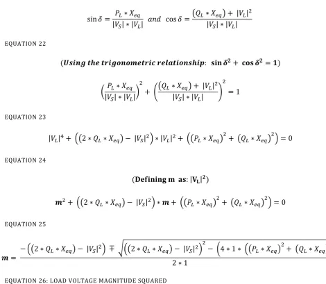
EQUATION 22
EQUATION 23
EQUATION 24
EQUATION 25
EQUATION 26: LOAD VOLTAGE MAGNITUDE SQUARED
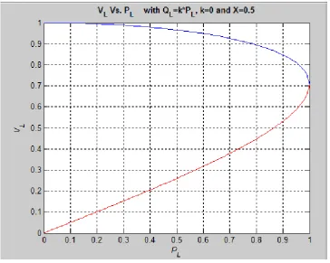
According to Equation 26, an increase in the load’s active power demand is initially accompanied by acceptable and fairly constant load voltages. In Figure 11, this operating region corresponds to the area where load active power is ≤ 0.3 per unit. However, above this active power demand, load voltage deteriorates sharply till it collapses. This relationship can be seen in Figure 11. A similar plot can be derived for the relationship between load voltage and load reactive power.
FIGURE 11: PLOT SHOWING VS FOR A SYSTEM WITH =0.5, =0 AND =1.0
As stated in [5], the stability-influencing factor for generators stems from the field and armature current limits. Armature current limits can be realized manually by network operators or
automatically via generator AVRs (Automatic Voltage Regulators). For field current limits, they are automatically determined by the generators overexcitation limiters (OXL). Regardless of which limit is first reached, both field and armature current limits sets the boundaries for reactive power
generation. When the load demands reactive power above the boundary set by either field or
Additionally from [5], voltage collapse is the situation where a low voltage profile (or bus voltage) is present in a significant part of a power distribution system. Unlike voltage instability, voltage collapse is not a single, immediate event. It is the end result of a sequence of undesirable events in the power distribution network; and these events can be triggered by voltage instability. Voltage collapse, coupled with unsuccessful system-recovery actions, can easily lead to a power blackout incident.
2.3.4
STABILITY ALGORITHMS
Stability algorithms are formulas that enable the derivation of scalar representations of a system’s stability. They are generally categorized according to the power system parameter that is used to detect stability indication. In this report, two categories of stability algorithms are presented. They are: Voltage Stability Algorithms and Line Stability Algorithms. As their name implies, voltage stability algorithms mostly relate voltage stability to system stability; whereas, line stability algorithms
measure the extent of a line’s stability and uses the result to estimate the overall system stability. It is important to note that these algorithms represent the extent of stability or instability by using accurate real-time system data. Thus, without the incorporation of synchrophasor devices, there would be no access to real-time data with the accuracy required to monitor system stability. The stability indices introduced below involve the some symbols. Definitions for these symbols are listed below.
2.3.4.1 VOLTAGE STABILITY INDICES
The need to accurately evaluate the stability of a power system pertaining to bus voltages is crucial. It is this need that spurred the development of voltage stability indices (VSI) or voltage collapse
proximity indices (VCPI). VSIs or VCPIs are indices that represent the voltage stability of a power system with scalar values. Depending on the type, properties and representation style such as upper and lower index limits, index sensitivity and complexity varies. However, most voltage stability indices represent voltage stability and collapse proximity with scalar values between 0 and 1. Among these are “Fast Voltage Stability Index”, “VCPI” and “VSI based on Maximum Power Transfers”. These are briefly reviewed in [12].
2.3.4.1.1 VSI BASED ON MAXIMUM POWER TRANSFERS (VSI)
As its title implies, this voltage stability index is based on the maximum transferable power of a system. As depicted in Equation 27, the stability index is derived from the ratio of the difference between maximum power and load bus power as seen from the perspective of the load. That is, the stability index is a representation of how well generated power is being transmitted to the load or the extent of how ‘lossless’ the system truly operates.
EQUATION 27: STABILITY INDEX VSI (BASED ON MAXIMUM POWER TRANSFER)
where:
EQUATION 28
EQUATION 29: MAXIMUM ACTIVE LOAD POWER
EQUATION 30: MAXIMUM REACTIVE LOAD POWER
Stability index values closer to zero (0) signifies a load bus voltage of marginal stability while stability index values closer to one (1) indicates that the bus voltage is stable. With the critical value being zero (0), a bus with stability index value less than or equal to zero (0) can be considered to have
experienced voltage collapsed.
2.3.4.1.2 FAST VOLTAGE STABILITY INDEX (FVSI)
This stability index is based on the power flow between two bus systems, similar to the previous algorithm. However, in [12], it is introduced as being predominantly line sensitive; hence, its use as a line stability index. According to [12], FVSI calculates line stability index by utilizing the algorithm presented in Equation 31.
EQUATION 31: STABILITY INDEX FVSI
2.3.4.1.3 INCREMENTAL REACTIVE POWER COST (IRPC)
Introduced in [14], the IRPC algorithm calculates a stability index based on the ratio between the change in the generator’s reactive power and the change in the load bus’s reactive power. It is defined in Equation 32 which also represents, in terms of generator’s reactive power, the cost required for each additional reactive load increase hence its name ‘Incremental Reactive Power Cost’.
EQUATION 32: STABILITY INDEX IRPC
where:
As the additional reactive power ‘cost’ increases, so does the instability of the system. Although it seems that each system has its own ‘cost’ margin; it can be inferred, from the system under analysis in [14], that its collapse margin is most likely three (3) while its maximum stability ‘cost’ is zero (0).
2.3.4.1.4 VOLTAGE COLLAPSE PROXIMITY INDEX (VCPI)
The Voltage Collapse Proximity Index, reviewed in [12], is based on the admittance matrix of a power system; and thus, does not require the development of a Thevenin equivalent system. However, it requires a modified voltage phasor; this is calculated based on the voltage phasor of all buses along with the admittance matrix. The collapse index is then calculated according to Equation 33.
EQUATION 33: STABILITY INDEX VCPI
where:
Collapse index values closer to one (1) indicates that the system is relatively unstable as the collapse margin is one (1). However, a collapse index of zero (0) signifies that the voltage at that particular bus is relatively stable and should not result in voltage collapse.
2.3.4.2 LINE STABILITY INDICES
Line stability indices are mainly developed for assessing the stability of transmission lines; in particular, power system branches between the generation and load bus. However, since they are based on fundamental electrical principles, they mirror the state of boundary buses.
2.3.4.2.1 LSI
Reviewed in [12], this line stability index; similarly named ‘Line Stability Index’, is based on the power flow of a two bus power network. It represents the stability of a line or its surrounding buses
according to Equation 34.
EQUATION 34: STABILITY INDEX LSI
where:
With stability index value of one (1) as the critical value, stability index values closer to one (1) indicates system branches or surrounding buses with low stability. Conversely, stability index values closer to zero (0) signifies branches or surrounding buses with relatively high stability. In essence, the lower the stability index, the higher the stability of the whole power system network.
2.4
THEVENIN EQUIVALENCE ALGORITHM
There are two generally accepted methods for the derivation of thevenin equivalent networks; one for relatively simple systems, the other for relatively complex systems.
FIGURE 12: A SIMPLE SYSTEM FOR THEVENIN CALCULATION
The first method is the more commonly known ‘open-circuit-voltage’ and ‘short-circuit-current’ method. In Figure 12, the common method to derive Thevenin equivalence is to calculate the easiest combination consisting of two of the required three thevenin parameters: ‘Thevenin Voltage’,
‘Thevenin Current’ and ‘Thevenin Impedance’. Hence, the thevenin equivalent circuit for Figure 12 can be obtained either by using Equation 35 and Equation 36, Equation 35 and Equation 37 or Equation 36 and Equation 37.
EQUATION 35: SIMPLE THEVENIN CALCULATION FOR IMPEDANCE
EQUATION 36: SIMPLE THEVENIN CALCULATION FOR LOAD VOLTAGE
EQUATION 37: SIMPLE THEVENIN CALCULATION FOR LINE CURRENT
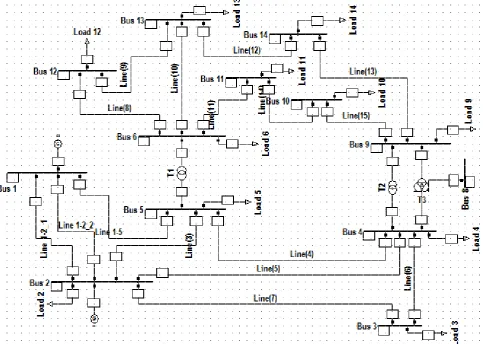
Now consider Figure 13. Due to the complexity of the power system network depicted in this figure, the thevenin method described above would not be recommended as it would not only be time consuming but prove to be difficult by hand calculations. Rather, the recommended method would be that of the thevenin equivalence algorithm. As its name implies, this algorithm is used to estimate thevenin equivalence parameters for a power system network; specifically, the thevenin equivalence source voltage and corresponding thevenin impedance. Reviewed in [13] and [12], the thevenin equivalence algorithm relies on the system’s admittance matrix in order to estimate a selected part of the power system. Pertaining to this project, this algorithm is essential because it allows for the minimization of synchrophasor locations by accurately estimating parts of the power system; thereby minimizing cost and data collection time. Additionally, due to the fact that it is based on the
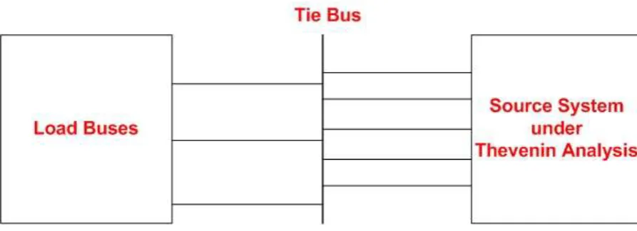
FIGURE 14: PERCEPTION OF THE THEVENIN EQUIVALENCE ALGORITHM
As shown in Figure 14, the thevenin equivalence algorithm is based on the assumption that system buses can be neatly partitioned into ‘Generator’, ‘Tie’ and ‘Load’ buses. The admittance matrix of such power system can be defined according to Equation 38. As shown in Equation 41 to Equation 43, further expansion of Equation 39 results in Equation 44 which defines the thevenin equivalent source voltage for a particular load with respect to other load voltages, load powers and connecting
admittances.
EQUATION 38: RELATIONSHIP BETWEEN CURRENT , VOLTAGE AND ADMITTANCE IN MATRIX FORM
(It is important to note that each element can be a vector as there can be multiple Load, Tie and
Generator Buses i.e. matrix)
EQUATION 39: LOAD VOLTAGE VECTOR
EQUATION 40: TIE VOLTAGE VECTOR
EQUATION 42: GENERAL EXPRESSION FOR LOAD VOLTAGE (JTH LOAD BUS)
EQUATION 43
EQUATION 44: THEVENIN EQUIVALENT SOURCE VOLTAGE
where:
Although the admittance matrix of a power system can be determined by implementing Kirchhoff’s Current Law or ‘KCL’ at nodes of interest, a ‘short-cut’ is provided in [15]. As implied from this method, there are 4 important steps that must be followed. There are:
1. Ensure that the circuit only contains admittances and independent current sources. To do this, the equivalent admittance circuit must be derived i.e. voltage sources with series impedance can be converted to current sources with parallel admittance, other impedances can be replaced with their equivalent admittances.
3. The ‘off-diagonal’ or non-diagonal terms are the negated admittances connected between the corresponding nodes i.e. between the row-node and corresponding column-node.
4. The elements of the left-hand current matrix are the current values injected into the corresponding node by the current sources.
2.5
SIMULATION PROGRAMS AND SOFTWARE
2.5.1
MATLAB BY MATHWORKS
Described as “…a high-level language and interactive environment for numerical computation,
visualization, and programming” [16], Matlab serves as the main computational software used during this project as it allowed for, among others, the easy implementation of complex mathematical algorithms such as those pertaining to power system stability and thevenin equivalence. As its becomes increasingly prominent due to its computational efficiency, other software such as
PowerFactory have made available means by which Matlab can be directly incorporated; essentially increasing the software’s adaptability, capability and user control.
2.5.2
POWERFACTORY BY DIGSILENT
As one of the two power system simulators utilized for the completion of this project, PowerFactory is a unique power simulator in that it allows data to be inputted and read in formats more commonly used in the power industry. For example, line data are per kilometers instead of per units.
Additionally, PowerFactory seems to be more suited to simulations involving transmission and distribution systems over several kilometers. Described as “…the leading electrical network analysis tool for applications in generation, transmission, distribution and industrial systems” [17],
Chapter 3:
STABILITY ANALYSIS USING STABILITY INDICES
As previously mentioned, this chapter is aimed at the verification, analysis and comparison of stability indices selected for use in later stages of this project. Although this is a verification stage, it is perhaps the most important stage of the project because it not only serves as an introduction to stability indices but also provides an insight to what can be expected pertaining to challenges and goal
attainment. Issues such as algorithm compatibility, interpretation and simulation complexities will be considered. Additionally, this chapter would provide sufficient information needed to evaluate algorithm efficiency at indicating system stability and allow a more accurate interpretation of algorithm indices.
This section details the major procedures involved in the completion of this stage. This includes test power networks, data accumulation, implementation, testing and analysis.
3.1
TEST NETWORKS
In order to accurately determine the effectiveness of selected stability indices, test data would be derived from 2 power networks. Shown in Figure 15 and Figure 16 are the test systems represented as single line diagrams via PowerWorld and PowerFactory. (System data are provided in sections 9.1 of the Appendix)
FIGURE 15: TEST POWER NETWORK 1
FIGURE 16: TEST POWER NETWORK 2 (IEEE ADAPTED [18] AND [19] )
The test power networks presented above should be sufficient for the verification of the selected stability indices as each embodies a unique topology.
3.1.1
TEST POWER NETWORK 1
Test power network 1, as depicted in Figure 15, consists of 2 Generators and 2 Loads, 1 Transmission line segment and 3 2-winding Transformers. The relatively simple topology of this 5-bus system allows for a better understanding of the stability algorithms and permitting for quick analysis or adjustment if necessary. As stated, system data such as bus voltages and element settings is given in section 9.1.1 of the Appendix.
3.1.2
TEST POWER NETWORK 2
2-winding Transformers. It is derived from the IEEE 9-bus test system. As stated, system data such as bus voltages and element settings is given in section 9.1.2 of the Appendix.
3.2
TEST CASES
For the appropriate verification of the stability indices selected; “VSI based on Maximum Power Transfers”, “Fast Voltage Stability Index” and “LSI”, a few scenarios would be used in order to simulate possible real-life scenarios. As mentioned previously, only cases relating to load power increase would be used for testing.
One possible trigger for voltage collapse is transmission line outage, which in itself, can be triggered by the tripping of breakers when a line overload occurs. Transmission line overloads occur when the demand power, that is, the power flowing through the transmission line, exceed the ratings of the line. An overloaded transmission line implies that a significant portion of the generated power is lost during transmission. It also signifies that the loss of other transmission lines in the power system is eminent if corrective actions aren’t taken.
Another common trigger for voltage collapse incidents is the increase in load demand to the point where the supply side struggles to meet this demand in power. This can occur in both active and reactive power. As explained in section 2.3.3.2, when load demand exceeds a critical power limit, both load voltage and power would experience a significant decrease. If not attended to, this decrease continues to a point where voltage collapse occurs.
However, as this chapter is aimed at simply testing and interpreting stability indices, only active and reactive load increase would be tested using the selected stability algorithms.
3.3
TASK IMPLEMENTATION
The implementation and verification of the voltage indices was mainly completed in MathWorks’ Matlab. Excluding data files compiled from PowerFactory simulation results, this task was completed via 3 major Matlab files. They are the ‘Main file’, the ‘Thevenin file’ and the ‘Stability Index files’; all of which are Matlab functions excluding the main file.
the ‘Stability Index files’ are function files containing the algorithm of the selected stability indices. Each stability algorithm is coded as a separate function; thereby enabling indices selection and, when necessary, a time efficient debugging process. Lastly, the ‘Main file’ serves as the control center for the verification process. It utilizes or ‘calls’ all other required files, including the aforementioned
functions, in order to successfully complete the verification process. The general procedure for each test system data and test cases are detailed below.
Data Acquisition – The ‘Main file’ is programmed to read specially formatted text files containing system data compiled from simulations completed in PowerFactory. As stated, these file includes source and load voltage(s), load power(s) and a system’s admittance matrix.
Thevenin source(s) and impedance(s) Derivation using the Thevenin Equivalence Algorithm encoded in the ‘Thevenin file’
Stability Indices Calculation – Deriving the system’s stability indices based on the three selected indices: VSI, FVSI and LSI.
Result, Analysis and Comparison – Based on the stability indices derived, a stability trend can be plotted. This plot, along with the P-V plot of the load bus in question, will be used to assess the sensitivity and accuracy of each of the selected stability indices.
As stated previously, Matlab was used in conjunction with PowerFactory for the simulation and collection of test system data in this report. (Matlab codes regarding the Main, Thevenin and Stability Indices files can be seen in section 9.3 of the Appendix).
3.4
RESULTS
The results presented below; Load 2 and 5 (referred to as 1 for simplicity) for tests power networks 1 and 2 respectively, were chosen because they highlight interesting aspects of each test network. However, a table of other load bus’s stability index values is provided in section 9.2 of the Appendix. It is important to recall; however, that each stability index was developed based on different
3.4.1
TEST POWER NETWORK 1
FIGURE 17: STABILITY PLOT DERIVED BY INCREASING LOAD 2’S REACTIVE POWER (10% INCREMENT OF INITIAL LOAD Q IN PER UNIT)
FIGURE 19: VOLTAGE-POWER PLOT SHOWING LOAD 2’S FINAL STATE IN RED (DURING 10% INCREMENT OF INITIAL LOAD P IN PER UNIT)
(Refer to section 5.4 for details on why the operating point is shown as being within, not on, the power curve)
Shown in Figure 17 and Figure 18 are the stability trends for load 2 while experiencing a 10%
increase in reactive and active power. This increase is based on the initial power value; that is, for the either power, 10% of said power’s initial value at Load 2’s bus is consecutively added.
For both power increment cases, all 3 stability algorithms indicate that the system is stable at the final power values (0.495pu for the reactive increment case and 0.66pu for the active increment case). This is because both power increment cases have a significantly high VSI value as well as significantly low FVSI and LSI values; and as stated in section 2.3.4, VSI reflects maximum stability with a value of 1 while LSI and FVSI reflects maximum system stability with values of 0.
In order to further verify this interpretation, the voltage-power plot shown in Figure 19 was
3.4.2
TEST POWER NETWORK 2
FIGURE 21: STABILITY PLOT DERIVED BY INCREASING LOAD 1’S ACTIVE POWER (10% INCREMENT OF INITIAL LOAD P IN PER UNIT)
FIGURE 22: VOLTAGE-POWER PLOT SHWOING LOAD 1’S FINAL STATE IN RED (DURING 10% INCREMENT OF INITIAL LOAD P IN PER UNIT)
(Refer to section 5.4 for details on why the operating point is shown as being within, not on, the power curve)
Similar to the results of test network 1, Figure 20 and Figure 21 show the stability trends for load 1 while experiencing a 10% increase in reactive and active power respectively. As previously stated, this implies that 10% of the varying power’s initial value at Load 1’s bus is consecutively added and the values are recorded and analyzed using VSI, FVSI and LSI.
In Figure 20 and Figure 21, VSI contradicts both FVSI and LSI as it indicates that the system is stable while the other two stability algorithms disagree. However, it is the VSI-derived stability values that are somewhat suspicious since it shows no change in system stability while either active or reactive power varies.
operating region is in the acceptable voltage-power region of the P-V curve. (Stability indices pertaining to the derived stability indices for both cases can be seen in section 9.2.2 of the Appendix)
3.5
ANALYSIS AND COMPARISON
In order to gain further insight regarding the effectiveness and sensitivity of the stability algorithms, it can be helpful to compare a few critical stability indices to their corresponding operating points. These are highlighted in Table 2.
TABLE 2: SOME OPERATING POINT PROPERTIES FOR TEST POWER NETWORKS 1 AND 2
System Name Load B us Power (per unit) Operating Point Properties
Test Power Network 1: Load 2 SBASE = 100 MVA
10% increment of: QINITIAL = 16.5 MVAr PINITIAL = 22 MW
0.22+0.165j (Initial) Reactive Load Manipulation
0.22+0.4785j
Real Load Manipulation 0.484+0.1650j
[60.13,6.879]% Gen Loading Reactive Load Manipulation
[80.94,13.67]% Gen Loading
[80.94,13.67,42.42]% Trans Loading Real Load Manipulation
[81.55,7.018]% Gen Loading
[81.55,36.84,50.19]% Trans Loading Test Power Network 2: Load 1
SBASE = 100 MVA 10% increment of: QINITIAL = 50 MVAr PINITIAL = 125 MW
1.25+0.5j + 0.5130 (Initial) Reactive Load Manipulation
1.25+1.0j + 0.5020
Real Load Manipulation 2.0+0.5j + 0.4138
[67.22,22.97,46.88]% Gen Loading Reactive Load Manipulation
[69.68,30.69,50.20]% Gen Loading 0.9480˂-10.56° pu V Load 1
Real Load Manipulation
[83.82,25.73,51.62]% Gen Loading [80.59,12.55,10.07]% Trans Loading
As presented in Table 2, Generator 1 for test power network 1 was initially operating at around 60% of its maximum power. When the reactive power demand rose to 0.4785 per units, Generator 1 was required to operate at 80% of its maximum power rating in order to supply the demanded power. However, as seen in the stability plot in section 3.4.1, all 3 stability algorithms indicated that Load 2’s bus was over 90% stable; and thus, implying that the overall system is stable.
algorithms. Going back through VSI, FVSI and LSI; Equation 27, Equation 31 and Equation 34 respectively, a few details stand out:
1) VSI is calculated as the minimum of three different power rations involving active, reactive and apparent power. It also takes into account the thevenin reactance of the system. Hence, VSI should be capable of representing any stability variations due to all 3 power forms as well as the transmission reactance of the system.
2) FVSI is predominantly reflective of stability changes due to a system’s reactive component; particularly, a system’s reactive power and thevenin reactance. Therefore, it is reasonable to expect FVSI to be an accurate reflection of any stability variation due to reactive components. On the other hand, it shouldn’t be shocking that FVSI may not be as accurate when
representing stability variations due to active components, for example, a change in the real or active power demand.
3) LSI; introduced as a line stability algorithm, produces stability results quite similar to FVSI. This is because LSI also considers both reactive power changes and thevenin reactance when deriving stability indices. However, unlike FVSI, LSI also takes into account changes in load power factor. This suggests that LSI should be more accurate than FVSI when representing stability variations due to voltage changes as well as real power changes.
However, the most important concept in the development of stability indices is that they are all based on reasonable assumptions i.e. constant load active power, constant load power factor and constant load reactive power. Based on these facts, it can be seen that not only are multiple stability indices required for an accurate assessment of system stability, the state of the system must be considered before the results from a stability index is acted upon. In test power network 2, the P-V curve was used to quickly check the current state of the system; and based on this, VSI was found to be more reflective of the system’s stability.
In a different situation, LSI or FVSI could have been more reflective of system stability as the situation may coincide with the fundamental assumption in the development of LSI or FVSI. Hence, as
Chapter 4:
STABILITY INDICES IN VOLTAGE REGULATION
With a better understanding of the tested stability indices, it becomes obvious that these indices can be advantageous when implemented into various transmission and distribution applications. One such application is the incorporation of stability indices in a system’s voltage regulation procedure. Voltage regulation refers to the process whereby bus voltage levels are maintained within an
appropriate boundary via regulatory devices such as capacitor banks and transformers. Since voltage regulation only aims to maintain voltage level, the inclusion of stability algorithms allows for the regulation of not only voltage levels but also system stability. However, it is important to remember that, as stability algorithms reflect system stability numerically, they require accurate, real-time system data. Hence, it becomes redundant to utilize stability algorithms in voltage regulation procedures without the inclusion of synchrophasor devices. This is because synchrophasor devices can accurately measure system data, transmit said data; and therefore, reliably monitor a system’s behavior.
Hence, it is only through the use of synchrophasor devices that stability algorithms can produce a reliably reflect a system’s stability. Likewise, it is only through the use of a reliable representation of system stability; synchrophasor-based stability algorithms, that the incorporation of stability algorithms in voltage regulation becomes worthwhile.
4.1
VOLTAGE REGULATION
Distribution networks have grown from being simply passive to being active. This implies that, as loads involving resistive and reactive components become more common, and significant fluctuations ensue due to the increase in renewable and distributed generation sources, power flow can no longer be seen as the simple flow from generation to load. Hence, it becomes a necessary for network operators to monitor voltage levels and ensure that they are kept within acceptable limits. Voltage regulation, according to [15], can be referred to as the percentage of voltage loss with respect to the voltage at the load bus, as defined by Equation 45. For an ideal power system network; zero voltage loss during transmission, the expected percentage regulation, as defined in Equation 45, is zero (0). In reality, it is near impossible to operate with zero (0) percentage regulation; besides, according to [20], a high steady state voltage can be just as detrimental to electrical equipment as a fluctuating voltage level. The aim is to maintain the voltage within the acceptable range.
This section focuses on the procedures required to regulate and control voltage at the load irrespective of power fluctuations and other load characteristics.
4.1.1
VOLTAGE REGULATION DEVICES
There are various devices developed to control and regulate voltage levels to within an acceptable range. Overviews of various regulatory methods are discussed in [21]; however, a brief description of some methods is provided in this section.
4.1.1.1 NETWORK RECONFIGURATION
According to [21], network reconfiguration for voltage regulation refers to opening or closing of
normal open points (NOP) between two radial feeders via relays. The closing of such points would
convert the ‘radial’ configuration of the system into a ‘ring’ configuration. Among others, the minimization of power loss throughout the system is an advantage of this regulation method. The reduction in lost power is achieved through the addition of ‘alternate’ paths created due to the ‘ring’ configuration. This allows for the mitigation of stability-deteriorating events such as transmission line overload.
However, as this is a relatively new method for voltage regulation, issues such as NOP positions, required NOP sequence under multiple power system operations and complex NOP structures incorporating other voltage regulation methods are still being tackled [21]. These are crucial issues since they determine the overall efficiency of this regulation method.
4.1.1.2 SHUNT CAPACITOR BANKS (SCB)
Capacitor banks produce reactive power; hence, a (shunt) capacitor bank generating similar reactive power magnitude as the load demands can significantly reduce the portion of apparent power that is transmitted as reactive power. Thus, allowing for further active power to be demanded, by the load, from the source.
FIGURE 23: AN EXAMPLE OF THE EFFECT OF A SHUNT CAPACITOR BANK (WHERE 0.45PU QL IS REQUIRED)
4.1.1.3 LOAD TAP CHANGERS (LTC)
Unlike capacitor banks which are sometimes referred to as ‘reactive generators’, Load Tap Changers do not specifically generate reactive power; rather, they simply step up or down primary voltage and current. They can directly manipulate load voltage by increasing or decreasing the transformer winding ratio or taps positions in order to increase or decrease the output voltage respectively. Although an ideal transformer does not consume power, real transformers have inductive elements that consume reactive power; thus, increasing the reactive power demand. However, since it allows for direct voltage manipulation by varying tap settings; and can therefore improve voltage profiles since power loss is reduced at a higher voltage, it is an essential part of power transmission and distribution. Additional reactive power consumed by the transformer can be dampened by a capacitor bank of similar reactive power ratings.
EQUATION 46: TRANSFORMER RELATIONSHIP BETWEEN VOLTAGE AND NUMBER OF WINDINGS
EQUATION 47: TRANSFORMER RELATIONSHIP BETWEEN CURRENT AND NUMBER OF WINDINGS
EQUATION 48: TRANSFORMER RELATIONSHIP BETWEEN IMPEDNACE AND NUMBER OF WINDINGS
EQUATION 49: TRANSFORMER VOLTAGE AFTER TAP CHANGE
where:
In order to avoid unnecessary tap changes during transient voltage fluctuations; normally known as ‘hunting’, time delays are usually allowed between tap changes. According to [21], a tap change takes about 3 to 10 minutes and several minutes interval between frequent operations is required when taking into account oxidisation in the tank oil.
One possible problem, with the use of SCBs and LTCs, is unnecessary switching. Either due to their respective dead-band or to the possibility of each being unaware of the other’s control impact, repetitive switching; or ‘hunting’, can occur in the power system. According to [22], synchrophasor incorporated devices; such as “SEL-487E Transformer Protection Relay and SEL-487V Capacitor Protection and Control System”, can eliminate hunting events by allowing for real-time data
4.2
PROPOSED STRUCTURE
FIGURE 24: STRUCTURE FOR VOLTAGE REGULATION PLUS STABILITY (SIMULATION)
4.3
EXAMPLE
FIGURE 25: SIMPLE 4-BUS SYSTEM TO BE USED AS EXAMPLE (NORMAL OPERATION: T2 TAP = 3 AND LOAD VOLTAGE = |0.9439| AT -5.8969°)
TABLE 3: DATA FOR EXAMPLE SYSTEM
Bus Voltages (Nominal) Elements and Properties
Bus 1 = 1pu (Base = 15kV L-L) T1 = Transformer, Z = 0.00299+0.0398j pu , Absoluteuk0 = 3%, Srated = 100MVA
Bus 2 = 1pu (Base = 132kV L-L) L1 = Line, Vrate = 132kV, Irate = 7.5kA, Z = 0.01938+0.1721j pu, CableType=Overhead
Bus 3 = 1pu (Base = 132kV L-L) T2 = Transformer, Z = 0.00299+0.0398j pu, Absoluteuk0 = 3%, Srated = 100MVA, Tap norm = 3, Tap low = 1, Tap high=9, Voltage per tap = 1%, Additional Phase Shift = 0°
Bus 4 = 1pu(Base = 11kV L-L) Load, P = 40MW, Q = 15MVar
As shown Figure 25, this example utilizes a simple 4-bus system. It is composed of a single Generator, 2 Transformers (T2 as Tap-changing), 1 Transmission line segment and 1 Load. This example will present one possible method of incorporating stability algorithm into voltage regulation procedure via the use of tap transformer T2 as the regulating device.
4.3.1
IMPLEMENTATION
model in order to avoid situations such as voltage hunting. In this example, load voltage will be modeled according to Equation 49 . A simulation of Transformer 2 (T2) under various tap changes will be completed in Matlab and the resulting load voltages and line currents will be used as inputs for the selected stability index in order to determine whether the current operating point provided both acceptable load voltage and acceptable voltage stability. In this example, only stability index VSI will be included in the voltage regulation procedure. The combined procedure will be simulated in Matlab.
(The corresponding Matlab file section are shown in section 9.3.1 of the Appendix)
4.3.2
RESULTS
The results tabulated below are the system’s optimum operating points under different scenarios such as the below-ideal load voltage state indicated in Figure 25, load increase events and load decrease events. Simulated in Matlab, the results show the advantageous outcomes of incorporating stability analysis methods into voltage regulation procedures. For the results below, the acceptable range for load voltage is selected as [0.96, 1.04].
TABLE 4: (MATLAB) TRANSFORMER TAP AND LOAD VOLTAGE UNDER VR+SI (INITIAL STATE AS IN FIGURE 25)
(Initial) – Vl (Initial) S- I (Initial) - Tap (VR+SI) - Vl (VR+SI) - SI (VR+SI) – Tap
0.9389 - 0.0970i 0.6369 3 0.9577 - 0.0989i 0.6369 5
TABLE 5: (MATLAB) TRANSFORMER TAP AND LOAD VOLTAGE UNDER VR+SI (LOAD POWER = 48MWW + 18MVAR)
(Initial) – Vl (Initial) S- I (Initial) - Tap (VR+SI) - Vl (VR+SI) - SI (VR+SI) – Tap
0.9230 - 0.1164i 0.5643 3 0.9599 - 0.1210i 0.5643 7
FIGURE 27: (POWERFACTORY) TRANSFORMER TAP AND LOAD VOLTAGE UNDER VR (LOAD POWER = 48MWW + 18MVAR)
The results above support the notion that; although transformer tap changes do not influence load voltage stability, the simple Matlab program (provided in section 9.3.1 of the Appendix) that simulates the stability indices-incorporated-voltage regulation (VR+SI) procedure suggest a transformer tap position that coincides with PowerFactory’s voltage regulation procedure. Hence, the incorporation of stability algorithms does not diminish the effectiveness of voltage regulation.
Additionally, the inclusion of stability algorithms as well as the step-by-step analysis method ensures that only regulatory device settings corresponding to the optimum combination of acceptable load voltages and stability indices are implemented in the system.
Moreover, it is obvious that by assessing the stability of possible operating points, an optimum operating point can be chosen. With the knowledge that stability indices can be used to assess the stability of an operating point; as confirmed in the previous chapter and the fact that various software have been developed to model and simulate power systems; PowerFactory for instance, it is clear that the proposed structure is feasible albeit with a clear condition for exiting the voltage regulation + stability procedure.
Chapter 5:
CHALLENGES AND RECOMMENDATIONS
Challenges encountered during the completion of this project are detailed below. Based on these challenges, some recommended actions are also detailed below.
5.1
SOFTWARE INTERCONNECTIVITY
The main software used in the completion of this project are PowerFactory and Matlab. PowerFactory was used to model and simulate power systems, and subsequently, use the results to represent synchrophasor measurements. Matlab was used to test and analyze stability indices by developing algorithms that corresponding to the selected stability indices.
However, in order to simulate the whole synchrophasor structure as shown in Figure 3, data derived from PowerFactory simulations had to be compiled and stored in a text file (see section 3.3). This text file acts as the input to the Matlab file which relies on the developed stability algorithms in order to analyze and graphically represent the stability trend of a particular system. Although it was
discovered during the course of this project that PowerFactory had in-built procedures to read and write data from and to Matlab, this procedures weren’t used due to their complexity.
Since the connection of both PowerFactory and Matlab will allow data to be exchanged between both software (pseudo-synchrophasor measurement device (PowerFactory) and analyses and visualization software (Matlab)) in real-time, further studies on Matlab’s and PowerFactory’s in-built procedures is recommended. With the ability to transmit data between PowerFactory and Matlab, there will be no need to store and compile system simulation result in a text file. Furthermore, this may allow for the possible segue between power system simulation (PowerFactory), system analysis and calculations including stability analysis (Matlab), and implementation in power system simulation
5.2
STABILITY INDICES
Although a fair understanding of stability indices was gained, it would be prudent to recommend further studies on their application on various power systems. This will allow for an even deeper understanding to be achieved; understanding that may even lead to further improvements on already-developed stability indices or the developments of an entirely new stability index.
Additionally, it is obvious that, since each stability index is developed based on different
characteristics of a power system, each stability index will possess different properties in terms of stability assessment and sensitivity. Consequently, the use of multiple stability indices is
recommended in the proposed incorporation into voltage regulation procedures. This method will ensure minimal error and would be sensitive to more stability-degrading events that occur in the power system.
5.3
SYNCHROPHASORS
Nowadays, almost all relays are capable of synchrophasor measurements since synchrophasors have been incorporated into their design. However, since this project is simulation-based, future studies on synchrophasor applications is recommended. This is because, in reality, unfortunate and unexpected developments may occur. Hence, further studies on actual synchrophasor applications will provide additional knowledge on how to react to these unfortunate developments and improving practical implementation skills. This may also give rise to more accurate methods of simulating power system scenarios involving synchrophasor devices and measurements.
5.4
SOFTWARE ACCURACY
Chapter 6:
FUTURE WORK
During the completion of this project, a few areas were noted to be in need of future development. As stated in the previous chapter, these areas include further research on stability indices and the real-time data exchange between computational software (Matlab) and power system simulation software (PowerFactory).
In order to reliably assess the stability of a system, it is recommended to use multiple stability indices and compare their results. However, as seen in section 3.4.2, stability indices do not always coincide with each other’s interpretation of the system’s stability. When one of the stability indices utilized give a significantly different indication of system stability, it defeats the purpose of increasing
assessment reliability through algorithm corroboration. Hence, it is important to fully understand the underlying stability indices as the problem may lie in the interpretation of its index. In this project, one of the future plans would be to research into stability indices VSI, FVSI and LSI in order to better determine how it was developed as well as methods to minimize interpr
![FIGURE 9: CLASSIFICATIONS OF POWER SYSTEM STABILITY (ADAPTED FROM [5])](https://thumb-us.123doks.com/thumbv2/123dok_us/90163.2010831/20.595.87.543.84.556/figure-classifications-power-stability-adapted.webp)