https://doi.org/10.5194/gmd-12-3523-2019 © Author(s) 2019. This work is distributed under the Creative Commons Attribution 4.0 License.
A parallel workflow implementation for PEST version 13.6 in
high-performance computing for WRF-Hydro version 5.0:
a case study over the midwestern United States
Jiali Wang1, Cheng Wang1, Vishwas Rao2, Andrew Orr1, Eugene Yan1, and Rao Kotamarthi1
1Environmental Science Division, Argonne National Laboratory, 9700 South Cass Avenue, Lemont, IL 60439, USA 2Mathematics and Computer Science Division, Argonne National Laboratory, 9700 South Cass Avenue,
Lemont, IL 60439, USA
Correspondence:Jiali Wang ([email protected]) and Rao Kotamarthi ([email protected]) Received: 10 October 2018 – Discussion started: 29 November 2018
Revised: 16 June 2019 – Accepted: 12 July 2019 – Published: 13 August 2019
Abstract. The Weather Research and Forecasting Hydro-logical (WRF-Hydro) system is a state-of-the-art numeri-cal model that models the entire hydrologinumeri-cal cycle based on physical principles. As with other hydrological mod-els, WRF-Hydro parameterizes many physical processes. Hence, WRF-Hydro needs to be calibrated to optimize its output with respect to observations for the application re-gion. When applied to a relatively large domain, both WRF-Hydro simulations and calibrations require intensive comput-ing resources and are best performed on multimode, multi-core high-performance computing (HPC) systems. Typically, each physics-based model requires a calibration process that works specifically with that model and is not transferrable to a different process or model. The parameter estimation tool (PEST) is a flexible and generic calibration tool that can be used in principle to calibrate any of these models. In its ex-isting configuration, however, PEST is not designed to work on the current generation of massively parallel HPC clusters. To address this issue, we ported the parallel PEST to HPCs and adapted it to work with WRF-Hydro. The porting in-volved writing scripts to modify the workflow for different workload managers and job schedulers, as well as to con-nect the parallel PEST to WRF-Hydro. To test the operational feasibility and the computational benefits of this first-of-its-kind HPC-enabled parallel PEST, we developed a case study using a flood in the midwestern United States in 2013. Re-sults on a problem involving the calibration of 22 parameters show that on the same computing resources used for paral-lel WRF-Hydro, the HPC-enabled paralparal-lel PEST can speed up the calibration process by a factor of up to 15 compared
with commonly used PEST in sequential mode. The speedup factor is expected to be greater with a larger calibration prob-lem (e.g., more parameters to be calibrated or a larger size of study area).
1 Introduction
thousands – of model simulations to understand how pertur-bations in model parameters affect simulations of dominant physical processes and to find the optimum value of a single parameter.
WRF-Hydro is a numerical model that can simulate the en-tire hydrological cycle using advanced high-resolution data such as satellite and radar products. Compared with the tra-ditional land-surface model (LSM) used by WRF, WRF-Hydro provides a framework for the multiscale representa-tion of surface flow, subsurface flow, channel routing, and baseflow, as well as a simple lake–reservoir routing scheme. As a physics-based model, WRF-Hydro includes many com-plicated physical processes that are nonlinear and must be parameterized. The default parameters given by WRF-Hydro may be valid for one region but not for another region. Hence, the calibration of related model parameters is often required in order to use the model in a new domain. In particular, for a large spatial domain such as the entire contiguous United States, in order to develop the optimal parameter sets in a rea-sonable amount of time, the calibration must be conducted on high-performance computing (HPC) systems in parallel instead of in sequential mode. To date, no such calibration tool can efficiently calibrate WRF-Hydro on HPC resources. Typically, each physics-based model needs a calibration code that is custom designed to work with that particular numer-ical model and its set of physics parameterizations, soft-ware architecture, and solvers. These custom-designed cali-bration codes are highly challenging and do not offer flexibil-ity. Therefore, a more flexible and generic calibration tool is needed that can calibrate any code that uses Message-Passing Interface–Open Multi-Processing (MPI–OpenMP) for paral-lelization on HPC systems.
One widely used generic and independent calibration tool is the parameter estimation tool (PEST). PEST (Doherty, 2016) conducts calibration automatically based on mathe-matical methods and is thus applicable for optimizing non-linear parameters. Compared with manual calibration, auto-matic calibration is more efficient and effective because it avoids interference from human factors (Madsen, 2000; Ge-tirana, 2010). The uniqueness of PEST is that it operates independently of models: there is no need to develop addi-tional programs for a particular model except preparing the files required by PEST (as described in Sect. 3.2). PEST has four modes of operation (Doherty, 2016). One of the modes is regularization mode, which supports the use of Tikhonov regularization and is found to be better for serving environ-mental models because, if implemented properly, it supports model predictions of minimum error variance, is numerically stable, and embraces rather than eschews the heterogeneity of natural systems. Singular value decomposition (SVD) can be used as a regularization device to guarantee the numerical stability of the calibration problem. The parallel PEST is able to distribute many runs across many computing nodes us-ing master–worker parallel programmus-ing. To our best knowl-edge, however, no approach is available that allows users
to submit jobs using PEST parallelization to a typical su-percomputing facility that uses job scheduling and work-load management such as Simple Linux Utility for Resource Management (SLURM), Portable Batch System (PBS), and Cobalt. A previous study (Senatore et al., 2015) used PEST to calibrate WRF-Hydro over the Crati River Basin in southern Italy. Because the study area was relatively small, the authors were able to conduct the calibration using PEST in sequential mode (Alfonso Senatore, personal communication, 2018).
The objective of this study is to (1) port the parallel PEST to HPC clusters operated by the U.S. Department of Energy (DOE) and adapt it to work with WRF-Hydro, (2) evaluate the performance of the HPC-enabled parallel PEST linked to WRF-Hydro by calibrating a flood event, and (3) explore the scale-up capability and computational benefits of the HPC-enabled parallel PEST by assigning different computing re-sources to the entire calibration process.
2 Model description 2.1 Study area
The case presented here is one of the worst floods experi-enced by greater Chicago area in the past 3 decades; the storm occurred on 18 April 2013. According to the National Weather Service (NWS), the heaviest 24 h accumulated rain-fall during this storm reached 201.4, 171.1, and 136.4 mm across Illinois, Iowa, and Missouri, respectively. The Mis-sissippi River crested at 10.8 m (1.7 m above flood stage), and the Illinois River crested in Peoria, Illinois, at 8.95 m; this river cresting broke the previous record of 8.78 m, set in 1943, and was 4.55 m above the historical normal river stage (NWS, 2013). Campos and Wang (2015) conducted three-domain nested WRF simulations to understand the dynam-ical and microphysdynam-ical mechanisms of the event. Our study builds on the smallest domain of that study, which covers Illi-nois and the majority of Iowa and Missouri at a spatial res-olution of 3 km (Fig. 1). The domain size is ∼495 000 km2 (747 km from west to east; 657 km from south to north). 2.2 WRF-Hydro configuration
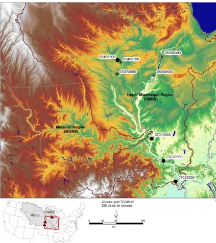
Figure 1.Eight USGS sites over the study area. The boundaries of the Upper Mississippi River Basin (UMRB) and Missouri River Basin (MORB) are highlighted. The four black circles indicate the sites that are used for calibrations; the four black crosses are sites that are used for transferability assessment. USGS site numbers corresponding to the site indices used in this study are as follows. Station 1: 05465500; Station 2: 07010000; Station 3: 07020500; Station 4: 07022000; Station 5: 05465700; Station 6: 05474000; Station 7: 05558300; Station 8: 05568500. The three inflow stations indicated by the black triangles on the lower left map are 06807000, 06887500, and 05389500.
et al., 2011). We utilize the Noah-MP LSM because com-pared with the Noah LSM it shows obvious improvements in reproducing surface fluxes, skin temperature over dry pe-riods, snow water equivalent, snow depth, and runoff (Niu et al., 2011). Noah-MP is configured at a grid spacing of 3 km, and the aggregation factor is 15; that is, starting from a 3 km LSM resolution in the domain shown in Fig. 1,
at-mospheric model. Overland flow, saturated subsurface flow, gridded channel routing, and a conceptual baseflow are active in this study. The gridded channel network uses an explicit, one-dimensional, variable time-stepping diffusive wave. The time step of 10 s also meets the Courant condition criteria for diffusive wave routing on a 200 m resolution grid. A direct output-equals-input “pass-through” relationship is adopted to estimate the baseflow. Although the baseflow module is not physically explicit, it is important because the water flow in the channel routing is contributed by both the overland flow and baseflow. If the overland flow is active as it is in this study, it passes water directly to the channel model. In this case the soil drainage is the only water resource flow-ing into the baseflow buckets. However, if the overland flow is deactivated but channel routing is still active, then WRF-Hydro collects excess surface infiltration water from the land model and passes this water into the baseflow bucket. This bucket then contributes the water from both overland and soil drainage to the channel flow. Therefore, the baseflow must be active if the overland flow is switched off. This study does not consider lakes and reservoirs.
We use the geographic information system (GIS) tool de-veloped by the WRF-Hydro team (Sampson and Gochis, 2018) to delineate the stream channel network, open-water (i.e., lake, reservoir, and ocean) grid cells, and groundwater– baseflow basins. Meteorological input for WRF-Hydro in-cludes hourly precipitation; near-surface air temperature, hu-midity, and wind speed; incoming shortwave and longwave radiation; and surface pressure. In this study, the hourly pre-cipitation is from the National Centers for Environmental Prediction (NCEP) Stage IV analysis at a spatial resolution of 4 km. The Stage IV data are based on combined radar and gauge data (Lin and Mitchell, 2005; Prat and Nelson, 2015) and have been shown to be temporally well correlated with high-quality measurements from individual gauges (see, e.g., Sapiano and Arkin, 2009; Prat and Nelson, 2015). The other hourly meteorological inputs are from the second phase of the multi-institution North American Land Data Assimila-tion System project, phase 2 (NLDAS-2) (Xia et al., 2012a, b), at a spatial resolution of 12 km. NLDAS-2 is an offline data assimilation system featuring uncoupled LSMs driven by observation-based atmospheric forcing.
During the 15 d period of this studied case, light to mod-erate rain occurred on 8 through 11 April 2013, followed by a relatively dry period from 12 to 15 April. Then a heavy rain event began on 16 April and peaked on 18 April. The heaviest rain band moved east of the study area on 19 April. The rainy event ended over the study area on 20 April (see Fig. S1 in the Supplement). We start the WRF-Hydro simu-lation on 1 October 2012 and run the model for 6 months to reach equilibrium. This 6-month period is considered spin-up time and is excluded from model calibration and eval-uation. We calibrate the river discharge calculated by the WRF-Hydro model from 00:00 UTC 9 April to 00:00 UTC 12 April 2013, considering it long enough to achieve our
ob-jective. We then evaluate the model performance against U.S. Geological Survey (USGS) observed river discharge from 00:00 UTC 12 April to 00:00 UTC 25 April 2013.
3 Calibration 3.1 Platforms
We customized the parallel PEST to work on three dif-ferent workload managers and job schedulers: SLURM at the National Energy Research Scientific Computing Center (NERSC), PBS at the Argonne National Laboratory Com-puting Resource Center (LCRC), and Cobalt at the Argonne Leadership Computing Facility. The tests presented here are conducted on Edison and Cori at NERSC and Bebop at Ar-gonne LCRC, which all use the SLURM workload manager and job scheduler.
The interface we have built between the parallel PEST and the management software is, in general, used for (1) set-ting the number of workers and the nodes for each worker to conduct a model run (WRF-Hydro here); (2) setting up the working directory for the workers; (3) finding the nodes that are available; (4) identifying the nodes that work for each worker; (5) passing the global files (the same for all the working directory) to all the workers (these files include the lookup table files that are not to be calibrated, the namelist files for both the LSM and hydrological sector, and restart files generated by the previous simulations or spin-up pe-riod); and (6) submitting the job for the entire calibration pro-cess, including the parallel PEST and parallel WRF-Hydro. The job can be submitted as a fresh run or as a restart in terms of the calibration process. The main difference for this inter-face on different management software is that different man-agement software has its own way to identify available nodes and to submit jobs. These differences require minor changes in the scripts we developed, which involves finding and iden-tifying available nodes for workers, and submitting jobs for the specific management software. See detailed comments in the published code and scripts.
3.2 PEST files and settings
that come from template files) and each model output file that PEST must read (such as frsxt_pts_out.txt). The man-agement file also sets the maximum running time for each worker. For workers that take longer than the maximum run-ning time, PEST will stop the model run by that particular worker and assign that model run to another worker if there is one with nothing else to do.
To the best of our knowledge, however, the parallel PEST is not designed to run on HPCs directly. We developed scripts and an interface to enable parallel PEST to run on HPCs using SLURM, PBS, or Cobalt workload managers and job schedulers. The development involved writing scripts to modify the workflow for different workload managers and job schedulers, as well as to connect the parallel PEST to WRF-Hydro. These developments enable parallel PEST to have many workers to run at the same time; each worker runs a parallel code (here WRF-Hydro) that uses more than one node, which could significantly reduce the wall-clock time for model calibrations. Although this master–worker paral-lelism may not be as efficient as a fully MPI approach, it is sufficient for model calibration and requires the least effort for the current parallel PEST to run on HPC systems.
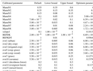
This study presents calibration results from PEST using SVD-based regularization mode to ensure numerical stability (Tonkin and Doherty, 2005). We focus on calibrating 22 pa-rameters (see Table 1 and a detailed description in Sect. 3.3) using 96 observation points and 22 items of prior information for the calibrated parameters. In each item of prior informa-tion, a value equal to its default value provided by WRF-Hydro v5.0 (or the log of its default value) is assigned for each adjustable parameter, assuming that default values are the preferred values. All prior information equations are as-signed a weight of 1.0. We asas-signed five different regulariza-tion groups to the prior informaregulariza-tion: Manning’s roughness coefficients specified by Strahler stream order in CHAN-PARM.TBL to one group; the parameters in HYDRO.TBL (Manning’s roughness coefficients for overland flow as a function of vegetation types) to another group; and three global parameters for Noah-MP – deep drainage (SLOPE), the infiltration scaling parameter (REFKDT), and saturated soil lateral conductivity (REFDK) – in GENPARM.TBL to the remaining three groups. The 96 observation points are given different weights based on the inversed mean of their observed discharge during the studied period (see the de-tailed description in Sect. 3.3 and 4.1). For a dede-tailed descrip-tion of these settings see the PEST user manual (Doherty, 2016).
3.3 Calibrated experiments
The primary objective of this study is to build a bridge for linking parallel PEST and WRF-Hydro on the basis of HPC clusters and to explore the computational benefits of this bridge. We do not attempt to extensively assess each indi-vidual tool or address questions in each indiindi-vidual domain,
such as optimizing the objective functions in PEST or cal-ibrating WRF-Hydro for a long time period considering all the relevant parameters to achieve an optimal parameter set. The calibration period thus is limited to only 3 d, which we believe is long enough to achieve our objective and to un-derstand WRF-Hydro’s sensitivity to the calibrated parame-ters. We calibrated WRF-Hydro using four USGS sites (re-ferred to as Station 1, Station 2, Station 3, and Station 4 hereafter), as shown in Fig. 1. (More USGS sites could be included if one manually reallocated the stations that were not properly assigned to the desired location on the channel network by the GIS tool.) As shown by the lower left index map in Fig. 1, the study area (the red box) only covers the lower part of the Upper Mississippi River Basin (UMRB) and a portion of the Missouri River Basin (MORB). In order to prepare observation datasets of streamflow contributedonly
Table 1.Calibrated 22 parameters and the optimum parameters found after five iterations based on the four USGS stations indicated by the solid circles in Fig. 1.∗
Calibrated parameter Default Lower bound Upper bound Optimum parameter
MannN1 0.55 0.35 0.6 0.6
MannN2 0.35 0.15 0.35 0.35
MannN3 0.15 0.08 0.15 0.15
MannN4 0.1 0.05 0.15 5.00×10⁻²
MannN5 7.00×10⁻² 0.02 0.1 6.59×10⁻²
MannN6 5.00×10⁻² 0.015 0.1 4.67×10⁻²
MannN7 4.00×10⁻² 0.01 0.08 2.24×10⁻²
MannN8 3.00×10⁻² 0.005 0.06 1.72×10⁻²
xslope1 0.1 1.00×10⁻⁴ 1 0.181358
REFDK 2.00×10⁻⁶ 1.00×10⁻⁸ 1.00×10⁻⁵ 6.69×10⁻⁷
REFKDT 1 0.01 5 0.956414
ovn1 (urban) 2.50×10⁻² 0.005 0.06 6.00×10⁻²
ovn2 (dry crop) 3.50×10⁻² 0.015 0.06 1.50×10⁻²
ovn3 (irrigated crop) 3.50×10⁻² 0.015 0.06 6.00×10⁻² ovn5 (crop–grass) 3.50×10⁻² 0.015 0.06 1.50×10⁻²
ovn6 (crop–wood) 6.80×10⁻² 0.035 0.25 3.68×10⁻²
ovn7 (grass) 5.50×10⁻² 0.015 0.25 0.127159
ovn10 (savanna) 5.50×10⁻² 0.015 0.3 0.157904
ovn11 (deciduous forest) 0.2 0.1 0.3 0.1
ovn14 (evergreen forest) 0.2 0.1 0.3 0.11768
ovn15 (mixed forest) 0.2 0.1 0.3 0.1
ovn16 (water) 5.00×10⁻³ 0.001 0.01 1.00×10⁻²
∗MannN numbers are the Manning’s roughness coefficients in CHANPARM.TBL; xslope1 is the first number of the nine SLOPE_DATA (deep drainage) in GENPARM.TBL; REFDK and REFKDT are saturated soil lateral conductivity and the infiltration scaling parameter, respectively, in GENPARM.TBL; ovn numbers are the Manning’s roughness coefficients for different land-use types.
its spatial variability, however) of overland roughness coef-ficients (OVROUGHRTFAC) rather than the actual value of each land type in the lookup table (e.g., Kerandi et al., 2018). Although this approach reduces the number of calibrated pa-rameters, it has less flexibility because changing one factor will change all the parameters that use the same proportion.
For the calibration exercises we conduct here, the reten-tion depth factor (RETDEPRTFAC) is fixed at 0.001. This value is reasonable because the modeled discharge of our particular configuration (Sect. 2.2) using default parameters is lower than observed discharge. Reducing this factor from 1 to 0.001 keeps less water in water ponds and more water on the surface so it can contribute to river discharge. First, we calibrate 48 parameters based on a 3 d simulation from 9 to 11 April 2013 (Table S1 in the Supplement). This calibration uses the estimation mode in PEST and considers an equal weight for all four USGS stations. We calibrate Manning’s roughness coefficients for both channels and land-use types, SLOPE, the REFKDT, and REFDK. Manning’s roughness coefficients control the hydrograph shape and the timing of the peaks; the SLOPE, REFKDT, and REFDK control the to-tal water volume. Second, based on the knowledge we learn from the 48-parameter calibration (see details in Sec. 4.1), for the same 3 d period, we reduce the number of calibrated
discharge that is modeled by using default parameters. Thus, we assign a higher weight (9.0) for Station 1 than for the other three stations (1.0) according to the inversed mean of observed discharge over these four stations in April 2013. The ratio of the weights between Station 1 and the other three stations stays similar even if the means are calculated based on different time periods.
3.4 Statistics
This study employs three statistical criteria: the Nash– Sutcliffe efficiency (NSE; Nash and Sutcliffe, 1970; Mori-asi et al., 2007), root mean square error (RMSE), and Pear-son correlation coefficient (PCC). RMSE and PCC evaluate model performance in terms of bias and temporal variation. NSE quantitatively describes the accuracy of modeled dis-charge compared with the mean of the observed data. Equa-tion (1) calculates the NSE with defined variables:
NSE=1− n P
t=0
Ytobs−Ytsim2
n P
t=0
Ytobs−Yobs mean
2
, (1)
where Ytobs is thetth observed value from USGS sites for river discharge, Ytsimis the tth simulated value from the WRF-Hydro output,Ymeanobs is the temporal average of USGS observed discharge, and n is the total number of observa-tion time points. An efficiency of 1 (NSE=1) corresponds to a perfect match between modeled discharge and observed data. An efficiency of 0 (NSE=0) indicates that the model predictions are as accurate as the mean of the observed data. An efficiency below zero (NSE<0) occurs when the model is worse than the observed mean. Essentially, the closer the NSE is to 1, the more accurate the model is.
4 Results
4.1 WRF-Hydro calibration and validation
Based on the knowledge we gained from the 48-parameter 3 d calibration, we adjust the range of critical parameters in the PEST control file to maintain their physical meanings. For example, we set the Manning’s roughness coefficient larger for stream order 1 than for stream order 2. We also ad-just the parameter range of the overland roughness coefficient for multiple land covers, such as cropland and forests. We exclude the parameters that are not sensitive to WRF-Hydro streamflow for this study in order to constrain the problem size due to the limits of computational resources. However, if one has an area of interest that is much larger with more land types than the study area here, then there would be more parameters to calibrate. Meanwhile, hundreds of constant pa-rameters in the Noah-MP model could affect the WRF-Hydro results (Cuntz et al., 2016) and can be calibrated as well. Both
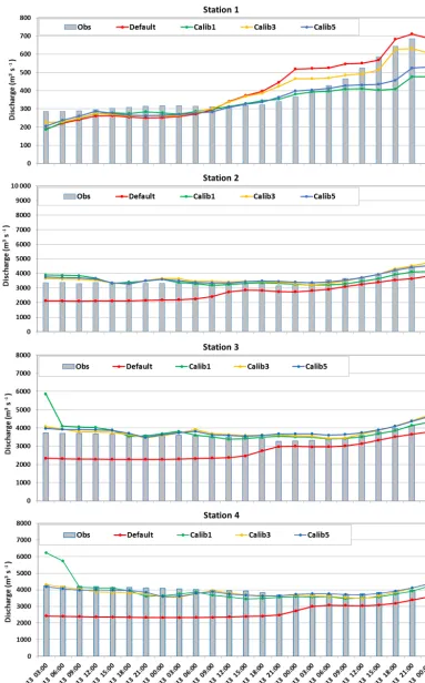
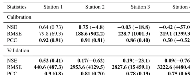
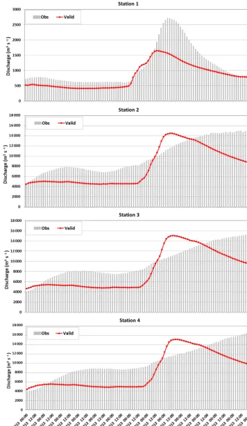
these situations would increase the burden of WRF-Hydro calibration. We perform the same 3 d calibration from 9 to 11 April 2013. Figure 2 shows the results of the 3 d mod-eled discharge using default and calibrated parameters after five iterations, as well as observed discharge. The four sta-tions are calibrated by considering different weights. While the model performance for Station 1 using the default and calibrated parameters is similar, the calibration improves the model performance over the drainage areas represented by Stations 2, 3, and 4 significantly. The modeled discharge us-ing the default parameter underestimates the streamflow by 24 %–33 %. PEST detects this underestimation, immediately adjusts the parameters, and increases the modeled discharge during the first iteration. After the third iteration, the differ-ence in calibrated results between different iterations is rel-atively small. We allow PEST to conduct five iterations and use the parameters obtained from the fifth iteration as our optimum parameters. As shown in Table 2, when the opti-mum parameters are used, the modeled discharges are much closer to the observations than the modeled results using de-fault parameters. The NSEs for the four stations increased from−4.8 (Station 2),−18.8 (Station 3), and −57.0 (Sta-tion 4) to 0.75,−0.03, and−0.42, respectively, being closer to 1. It is noteworthy that although NSE values between 0.5 and 0.65 have been suggested to indicate a model of suffi-cient quality, we see much lower NSE values for Stations 3 and 4 with calibration results close to the observations. This may be because the objective function used in PEST is the sum of squared weighted residuals (SSWR), which is calcu-lated differently from NSE. Thus even if SSWR reaches a small value, the NSE might still be far from 0.5. Incorporat-ing other measures into the objective function of PEST may improve the robustness of PEST calibrations. The RMSEs decreased from 902.2, 1001.3, and 1399.3 m3s−1to 188.6, 228.7, and 219.1 m3s−1, respectively.
Table 2.Statistics of model performance using optimum and default (in parentheses) parameters for Stations 1–4 during the calibration and validation period.∗
Statistics Station 1 Station 2 Station 3 Station 4
Calibration
NSE 0.64 (0.73) 0.75(−4.8) −0.03(−18.8) −0.42(−57.0) RMSE 79.8 (69.3) 188.6 (902.2) 228.7 (1001.3) 219.1 (1399.3)
PCC 0.92 (0.91) 0.91 (0.81) 0.86 (0.40) 0.50(−0.52) Validation
NSE 0.52 (0.41) 0.17(−0.62) 0.19(−23.1) 0.09(−0.76) RMSE 440.6 (487.3) 2953.6 (4129.5) 2827.6 (15 459.1) 3222.6 (4480.4)
PCC 0.9 (0.8) 0.81 (0.70) 0.78 (0.19) 0.75 (0.65)
∗The calibration is for 3 d (9–11 April) and includes 22 parameters. The validation period is 12–24 April. Bold typeface indicates the calibrated model results are closer to observations compared with the default model results. NSE and PCC are unitless (RMSE: m3s−1).
much discharge to the channels in a long-term view, as is also true for the other three large river stations. As a re-sult, the contribution from the baseflow to the river discharge in model simulations does not stay as long as in real situa-tions. In the observations, the river discharge decreases from the peak at a speed of ∼500 m3s−1d−1, while the mod-eled river discharge decreases from the peak at a speed of ∼1667 m3s−1d−1. Using an exponential storage–discharge function for the baseflow may improve this situation. Other reasons include the fact that the parameter range we set in the PEST control file is perhaps not wide enough, as we can see from Table 1 that several optimal parameters hit the bound of parameter ranges. Allowing wider parameter ranges may improve the calibration results.
Alternatively, instead of calibrating the stations that have large drainage areas and water coming from outside the cur-rent model domain, we have also tested calibrating small flows at local stations that have relatively small drainage ar-eas covered by the current study area. This requires gener-ating a new high-resolution GIS data file to distribute the stations of interest. We first run the WRF-Hydro model for 6 months using default parameters to spin up the model, and then we calibrate the model based on observations of these local stations. Results including figures and tables are shown in the Supplement. The calibration results are improved com-pared to the results that use default parameters, although fur-ther improvements are still needed. This again may be be-cause the parameter range is not wide enough to consider the possible values of parameters that work for these specific areas represented at local stations, as we see many optimal parameters hit the bound of the parameter range. More tests to figure out a better set of parameters are needed for future investigation, which is beyond the scope of this study.
4.2 Computational benefits of parallel PEST on HPCs
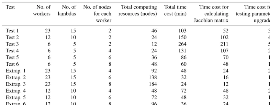
Table 3.Experiments designed to test the scale-up capability and computational benefits of the HPC-enabled parallel PEST linked to WRF-Hydro.∗
Test No. of No. of No. of nodes Total computing Total time Time cost for Time cost for workers lambdas for each resources (nodes) cost (min) calculating testing parameter
worker Jacobian matrix upgrades
Test 1 23 15 2 46 103 52 51
Test 2 12 10 2 24 150 102 48
Test 3 6 5 2 12 264 211 53
Test 4 6 5 4 24 131 107 24
Test 5 6 5 6 36 86 70 16
Test 6 6 5 8 48 60 48 12
Extrap. 1 23 15 4 92 48 24 24
Extrap. 2 23 15 6 138 32 16 16
Extrap. 3 23 15 8 184 24 12 12
Extrap. 4 12 10 4 48 72 48 24
Extrap. 5 12 10 6 72 48 32 16
Extrap. 6 12 10 8 96 36 24 12
∗The tests were conducted on Edison at NERSC. Edison is a Cray XC30 with a peak performance of 2.57 petaflops per second. It has 5586 nodes, 24 cores per node, and∼61GB of physical memory per node.
In this study we test the computational performance of the HPC-enabled parallel PEST using different numbers of workers (6, 12, and 23) for the 22-parameter calibration. As shown in Table 3, we conducted six experiments: Test 1 uses 23 workers, Test 2 uses 12 workers, and Test 3 uses 6 work-ers. All three tests use two nodes for each worker to run WRF-Hydro in parallel. The maximum number of lambda-testing runs undertaken per iteration is set to 15, 10, and 5 for Tests 1, 2, and 3, respectively, to ensure that only one cycle of WRF-Hydro runs is devoted (using 15, 10, and 5 work-ers from Tests 1, 2, and 3, respectively) to testing Marquardt lambdas. Note that the maximum number of lambda-testing runs should be set equal to or less than the number of work-ers available. Otherwise, another cycle of WRF-Hydro runs needs to be conducted. In fact, generating more Marquardt lambdas does not always guarantee that the best Marquardt lambdas are generated. In contrast, it may make the model convergence slower (here, PEST) or even lead to model fail-ure.
In order to test the trade-offs between the computing nodes used for running parallel WRF-Hydro and the workers used for running parallel PEST, Tests 4, 5, and 6 use the same number of workers (six) as Test 3 but use different numbers of nodes for each worker to run WRF-Hydro in parallel. Ex-plicitly, Test 4 uses four nodes per worker, Test 5 uses six nodes per worker, and Test 6 uses eight nodes per worker. The maximum number of lambda-testing runs undertaken per iteration is set to five for Tests 4, 5, and 6. Note that the time costs in Table 3 are limited to only one iteration. Con-ducting more iterations will increase the cost of wall-clock time and computing resources but will not change the con-clusion for the scale-up capability and computational benefits for the HPC-enabled parallel PEST linked to WRF-Hydro.
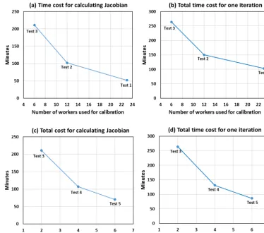
Figure 4.Time cost for calculating the Jacobian matrix and total time cost for one iteration for five experiments (see Table 3) using different numbers of workers to conduct PEST(a, b)and different numbers of nodes for each worker(c, d)to conduct WRF-Hydro.
using the same number of nodes for running parallel WRF-Hydro, we can estimate the computing speedup by assuming an increase in the number of calibrated parameters to 50. This would be the case, for example, to evaluate model sensitive-ness to the physics in Noah-MP or the spatial variabilities of certain parameters. We then expect to use 51 workers to cal-culate the Jacobian matrix in only one cycle. This would then be 28–30 times faster than running PEST using one worker (or in sequential mode). Similarly, if 100 parameters were used for the calibration for the same case study, a factor of up to 60 speedup in the calibration process would be achieved by running the HPC-enabled parallel PEST.
In addition, by increasing the number of nodes for each worker to conduct WRF-Hydro (Tests 3, 4, 5, and 6), the time cost for the entire calibration process is significantly re-duced (Fig. 4c and d). Specifically, WRF-Hydro scales up well when using four, six, and eight nodes, and thus both the time spent on calculating the Jacobian matrix and the time spent on testing the parameter upgrades are decreased by 49 %, 67 %, and 77 %, respectively, when using four, six, and eight nodes compared with using two nodes. Therefore, the total time spent is also decreased when using more nodes
for each worker (see Table 3). Moreover, if one has a larger study area, such as the entire contiguous United States, we expect WRF-Hydro to have an even better scale-up capabil-ity (e.g., on dozens of nodes) than in this study.
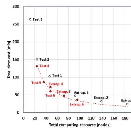
As shown in Fig. 5, compared with Test 3 (which requires the fewest computing resources – 12 nodes in total), hav-ing more workers (with the same number of nodes for each worker, e.g., Tests 1 and 2) takes more time than the ideal curve. The ideal curve assumes a linear speedup based on the time cost of Test 3. However, using the same number of workers and increasing the number of nodes for each worker (e.g., Tests 4, 5, and 6) can achieve the ideal speedup. Even when using 12 workers, increasing the number of nodes for each worker can still achieve a speedup close to the ideal curve (Extrap. 4, 5, and 6). Using 23 workers and increas-ing the number of nodes for each worker will not achieve the ideal speedup (Extrap. 1, 2, and 3). Therefore, if one only has a certain number of nodes available, we recommend us-ing a relatively small number of workers but a large number of nodes for each worker. For example, if one has 48 nodes, then there are three options that can be considered: using 23 workers and two nodes per worker; using 12 workers and four nodes per worker; and using 6 workers and eight nodes per worker. Other partitions (16×3; or 8×6) between num-bers of workers and nodes per worker are not as efficient as above. These three options will cost 103, 72, and 60 min, re-spectively, to finish one iteration. Thus, using six workers and eight nodes per worker is the most efficient way to spend the limited computing resources. On the other hand, if one would like to conduct the calibration in a short time period without any limits for the computing resources, then using 23 workers and eight nodes (perhaps even more nodes depend-ing on the scale-up capability of WRF-Hydro) will finish one iteration in∼24 min.
4.3 Evaluation of spatial transferability of the calibrated parameters
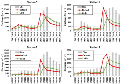
To assess the transferability of the calibrated parameters, we apply the optimum parameters obtained from the calibration for the four stations (black circles) in Fig. 1 to another set of four stations (crosses in Fig. 1) in the study area. All four sites are located on relatively small rivers, so the lag time be-tween precipitation peak and discharge peak is much shorter than that for Stations 2, 3, and 4. The assessment compares the observed discharge with the closest grid cells from the discharge output of WRF-Hydro. Figure 6 shows the ob-served and modeled discharge using the default and opti-mum parameters. Overall, WRF-Hydro’s default parameters underestimate the discharge and misrepresent the timing of discharge peaks compared with observations over the four assessed stations (Stations 5, 6, 7, and 8). By using the cal-ibrated parameters from other sites over the area, the model results increase the discharge and shift the hydrograph shape so they are much closer to the observations than model re-sults using default parameters. The absolute error of simu-lated discharge decreases by 13.1 %, 38.3 %, and 71.6 %, re-spectively, over Stations 6 through 8 (Station 5 shows a 6 % increase in absolute error) compared with the default
simu-Figure 5.Total time cost and total computing resources needed for each test and extrapolated scenario, which use different numbers of workers and different numbers of nodes per worker. The dash line is an ideal curve, which assumes a linear decrease in terms of time cost when more computing resources are used, built on Test 3. All the circles are real costs for time and computing resources for each test and extrapolated scenario. The red text and filled circles indicate that those specific tests meet the ideal speedup curve.
lated discharge. We also find that using SVD-based regular-ization for the PEST calibration captures the timing of the discharge peak better than using the estimation mode, which is 1 d earlier than the observations in reaching the discharge peak.
5 Summary and discussion
Figure 6. Observed and modeled daily averaged discharge (m3s−1) over the four stations indicated by the black crosses in Fig. 1 for 9–24 April using the default and optimum parameters (shown in Table 1) identified by the 3 d calibration.
the performance of calibrated WRF-Hydro against observa-tions in hydrograph features, such as the volume and timing of flood events. We examine the scale-up capability and putational benefits of the tool by assigning different com-puting resources for PEST and for WRF-Hydro. While this study presents the optimum parameters identified from the calibration of the particular flood event, the parameters can be significantly different if one uses different physics, such as an exponential storage–discharge function for a ground-water model or reach-based channel routing. Our preliminary testing shows that using exponential storage-discharge func-tion with the default parameters provided by WRF-Hydro, the modeled discharge was larger than that of observations for this particular study. Thus, the calibration will need to adjust the parameters to reduce the discharge. Our study finds that for calibrating 22 parameters, using the same com-puting resources for running WRF-Hydro, the HPC-enabled PEST calibration tool can speed up WRF-Hydro calibration by a factor of 15 compared with running PEST in sequential mode. The speedup factor can be larger when there are more parameters to be calibrated.
The following are several key points that we would like to highlight and to inform future studies.
1. In this study, we consider using the prior or regulariza-tion informaregulariza-tion only for the parameters that we cali-brate. As is the case with solving inverse problems, prior
information is added to improve the smoothness of the solutions. In order to build a more comprehensive cal-ibration, an important aspect that can be considered is to enrich the prior with available historical data (e.g., April and May from the past few years). Hence, the reg-ularization objective function in PEST will constitute not only the discrepancies between parameters and their “current estimates” but also the discrepancies between WRF-Hydro simulations and preferred values (which is the observed time series of historical discharge). Ad-ditionally, one can use the pilot-points technique de-scribed by Doherty (2005) in conjunction with parame-ter estimation to add more flexibility to the calibration process. This will be potentially beneficial in improving the predictions.
parame-ters (when compiled with SPATIAL_SOIL=1). Cali-brating these spatial parameters based on the grid scale (e.g., catchments) rather than a single value will give the model more flexibility and may thus better fit the obser-vations (Hundecha and Bardossy, 2004; Wagener and Wheater, 2006). In practice, for example, one can in-clude regional OVROUGHRTFACs (e.g., their lower– upper bounds and default values) in the PEST control file based on catchments. However, the selection of the locations and sizes of catchments may introduce signif-icant uncertainties to the calibration results, which re-quire systematic and comprehensive investigation and understanding of the study area.
3. This study is limited to calibrating the observed stream-flow only based on the format of one of the WRF-Hydro model outputs for individual stations (frxst_pts_out.txt). It is feasible, however, to calibrate other variables as long as the observation data are available. For example, one can either find the closest point from the gridded output (of WRF-Hydro) to the observation location and then compare that model grid to observations, or one can change the WRF-Hydro input–output code to out-put other variables in the frxst_pts_out.txt file, so they can still use the same interface we developed here to calibrate other variables in addition to the discharge. 4. The optimal parameter set obtained from this study is
from the fifth iteration of parallel PEST by testing five Marquardt lambdas. Testing different numbers of lamb-das or calibrating different numbers of parameters may generate a different set of optimal parameters. These pa-rameter sets can all make physical sense and be equally good for reproducing observed discharges. This phe-nomenon is called equifinality (Beven and Freer, 2001; Savenije, 2001), which is an important source of model uncertainty. To reduce the model uncertainty by reduc-ing the equifinality, hydrologists carry out additional modeling objectives for model evaluation to find more useful parameter sets (Mo and Beven, 2004; Gallart et al., 2007). Alternatively, inspired by no. 3 discussed above, one can calibrate the WRF-Hydro model based on more than one variable, such as discharge and soil moisture (or heat flux or water table depth), to reduce the number of optimal parameter sets and thus reduce the model uncertainty of predictions for these variables. 5. While this study ported the parallel PEST to an HPC system and linked it to WRF-Hydro, we note that BEOPEST is available in the PEST family. BEOPEST has the same functionality as parallel PEST but uses a different approach for communication between mas-ter and workers. Working with HPC-enabled BEOPEST may save total time cost since BEOPEST uses the Transmission Control Protocol and the Internet Proto-col instead of message files (reading input and writing
output between master and workers) for communica-tion. We expect it to be relatively straightforward to use BEOPEST to calibrate WRF-Hydro on HPCs since the interface remains the same, except one needs to copy the template and instruction files in addition to the global files (see Sect. 3.1) into each working folder.
Code and data availability. The observed river discharge is down-loaded from the USGS Surface-Water Data website, available at https://waterdata.usgs.gov/nwis/sw (last access: 26 January 2018). The Stage IV precipitation data were downloaded from https://data. eol.ucar.edu/dataset/21.093 (last access: 17 January 2018). PEST was downloaded from http://www.pesthomepage.org/Downloads. php (last access: 1 May 2018). We use the Unix PEST version 13.6. The scripts and files that are developed in this study and required by PEST for calibrating WRF-Hydro are available at https://doi.org/10.5281/zenodo.3247116 (Wang et al., 2019).
Supplement. The supplement related to this article is available on-line at: https://doi.org/10.5194/gmd-12-3523-2019-supplement.
Author contributions. JW proposed the project and developed the study case in WRF and WRF-Hydro. CW developed the scripts and code to port parallel PEST to DOE supercomputers and adapt it to work with WRF-Hydro. VR provided important input for the regularization calibration method. AO operated the ArcGIS tool to delineate the high-resolution grid cells to include stream chan-nel network, open water, and groundwater and baseflow basins. EY provided important input for hydrology during the revision of this paper. RK provided high-level guidance and insight for the entire project. All authors commented on this paper.
Competing interests. The authors declare that they have no conflict of interest.
Acknowledgements. Computational resources are provided by the DOE-supported National Energy Research Scientific Computing Center, Argonne National Laboratory Computing Resource Center, and Argonne Leadership Computing Facility. Our special thanks to the PEST developers and the entire WRF-Hydro team, especially Kevin Sampson for his guidance on the ArcGIS tool. We gratefully thank the two reviewers for their valuable comments and sugges-tions, which tremendously improved this paper.
Financial support. This research has been supported by a Labo-ratory Directed Research and Development (LDRD) Program at Argonne National Laboratory through U.S. Department of Energy (DOE) contract DE-AC02-06CH11357.
References
Arnault, J., Wagner, S., Rummler, T., Fersch, B., Bliefernicht, J., Andresen, S., and Kunstmann, H.: Role of runoff–infiltration par-titioning and resolved overland flow on land–atmosphere feed-backs: A case study with the WRF-Hydro coupled modeling sys-tem for West Africa, J. Hydrometeorol., 17, 1489–1516, 2016. Beven, K. and Freer, J.: Equifinality, data assimilation, and
uncer-tainty estimation in mechanistic modelling of complex environ-mental systems using the GLUE methodology, J. Hydrol., 249, 11–29, 2001.
Campos, E. and Wang, J.: Numerical simulation and analysis of the April 2013 Chicago Floods, J. Hydrol., 531, 454–474, 2015. Chen, F. and Dudhia, J.: Coupling an advanced land
surface-hydrology model with the Penn State-NCAR MM5 modeling system, Part I: Model implementation and sensitivity, Mon. Weather Rev., 129, 569–585, 2001.
Cuntz, M., Mai, J., Samaniego, L., Clark, M., Wulfmeyer, V., Branch, O., Attinger, S., and Thober, S.: The impact of standard and hard-coded parameters on the hydrologic fluxes in the Noah-MP land surface model, J. Geophys. Res.-Atmos., 121, 10676– 10700, https://doi.org/10.1002/2016JD025097, 2016.
Doherty, J.: Ground water model calibration using pilot points and regularization, Groundwater, 41, 170–177, 2005.
Doherty, J.: PEST: Model Independent Parameter Estimation, User Manual, 6th ed., Watermark Numerical Computing, Brisbane, Queensland, Australia, 2016.
Gallart, F., Latron, J., Llorens, P., and Beven, K. J.: Using internal catchment information to reduce the uncertainty of discharge and baseflow predictions, Adv. Water Resour., 30, 808–823, 2007. Getirana, A. C. V.: Integrating spatial altimetry data into the
auto-matic calibration of hydrological models, J. Hydrol., 387, 244– 255, https://doi.org/10.1016/j.jhydrol.2010.04.013, 2010. Gochis, D. J., Barlage, M., Dugger, A., FitzGerald, K., Karsten, L.,
McAllister, M., McCreight, J., Mills, J., RafieeiNasab, A., Read, L., Sampson, K., Yates, D., and Yu, W.: The WRF-Hydro mod-eling system technical description, (Version 5.0). NCAR Techni-cal Note. 107 pp., available at: https://ral.ucar.edu/projects/wrf_ hydro/technical-description-user-guide, last access: 1 June 2018. Hundecha, Y. and Bárdossy, A.: Modeling of the effect of land use changes on the runoff generation of a river basin through pa-rameter regionalization of a watershed model, J. Hydrol., 292, 281–295, 2004.
Kerandi, N., Arnault, J., Laux, P., Wagner, S., Kitheka, J., and Kunstmann, H.: Joint atmospheric-terrestrial water balances for East Africa: A WRF-Hydro case study for the upper Tana River basin, Theor. Appl. Climatol., 131, 1337–1355, https://doi.org/10.1007/s00704-017-2050-8, 2018.
Lin, Y. and Mitchell, K. E.: The NCEP stage II/IV hourly precip-itation analyses: Development and applications, Preprints, 19th Conf. on Hydrology, 10 January 2005, San Diego, CA, USA, Amer. Meteor. Soc., 1.2., 2005.
Madsen, H.: Automatic calibration of a conceptual rainfall–runoff model using multiple objectives, J. Hydrol., 235, 276–288, 2000. Mo, X. and Beven, K.: Multi-objective parameter conditioning of a three-source wheat canopy model, Agr. Forest Meteorol., 122, 39–63, 2004.
Moriasi, D. N., Arnold, J. G., Van Liew, M. W., Bingner, R. L., Harmel, R. D., and Veith, T. L.: Model evaluation guidelines for
systematic quantification of accuracy in watershed simulations, T. ASABE, 50, 885–900, 2007.
Nash, J. E. and Sutcliffe, J. V.: River flow forecasting through con-ceptual models, part I – A discussion of principles, J. Hydrol., 10, 282–290, https://doi.org/10.1016/0022-1694(70)90255-6, 1970. Niu, G.-Y., Yang, Z.-L., Mitchell, K. E., Chen, F., Ek,
M. B., Barlage, M., Kumar, A., Manning, K., Niyogi, D., Rosero, E., Tewari, M., and Xia, Y.: The commu-nity Noah land surface model with multiparameterization op-tions (Noah-MP): 1. Model description and evaluation with local-scale measurements, J. Geophys. Res., 116, D12109, https://doi.org/10.1029/2010JD015139, 2011.
NWS (National Weather Service): Record river flooding of April 2013, available at: https://www.weather.gov/ilx/ apr2013flooding, last access: 2 May 2013.
Prat, O. P. and Nelson, B. R.: Evaluation of precipitation estimates over CONUS derived from satellite, radar, and rain gauge data sets at daily to annual scales (2002–2012), Hydrol. Earth Syst. Sci., 19, 2037–2056, https://doi.org/10.5194/hess-19-2037-2015, 2015.
Sampson, K. and Gochis, D.: WRF Hydro GIS Pre-processing tools, Version 5.0 Documentation, NCAR Technical Note, 45 pp., available at: https://ral.ucar.edu/projects/wrf_hydro/ pre-processing-tools (last access: 17 January 2017), 2018. Sapiano, M. R. P. and Arkin, P.A.: An intercomparison and
validation of high-resolution satellite precipitation estimates with 3-hourly gauge data, J. Hydrometeor., 10, 149–166, https://doi.org/10.1175/2008JHM1052.1, 2009.
Savenije, H. H. G.: Equifinality, a blessing in disguise?, Hydrol. Process., 15, 2835–2838, 2001.
Senatore, A., Mendicino, G., Gochis, D. J., Yu, W., Yates, D. N., and Kunstmann, H.: Fully coupled atmosphere-hydrology simulations for the central Mediterranean: Im-pact of enhanced hydrological parameterization for short and long time scales, J. Adv. Model. Earth Sy., 7, 1693–1715, https://doi.org/10.1002/2015MS000510, 2015.
Soong, D. T., Prater, C. D., Halfar, T. M., and Wobig, L. A.: Man-ning’s roughness coefficients for Illinois streams, U.S. Geologi-cal Survey Data Series 668, U.S. GeologiGeologi-cal Survey, Reston, Vir-ginia, USA, 2012.
Tonkin, M. J. and Doherty, J.: A hybrid regularized in-version methodology for highly parameterized envi-ronmental models, Water Resour. Res., 41, W10412, https://doi.org/10.1029/2005WR003995, 2005.
Wagener, T. and Wheater, H. S.: Parameter estimation and region-alization for continuous rainfall-runoff models including uncer-tainty, J. Hydrol., 320, 132–154, 2006.
Wang, J., Wang, C., Orr, A., and Kotamarthi, R.: A par-allel workflow implementation for PEST version 13.6 in high-performance computing for WRF-Hydro version 5.0: a case study over the Midwestern United States, Zenodo, https://doi.org/10.5281/zenodo.3247116, 2019.
ap-plication of model products, J. Geophys. Res., 117, D03109, https://doi.org/10.1029/2011JD016048, 2012a.
Xia, Y., Mitchell, K., Ek, M., Cosgrove, B., Sheffield, J., Luo, L., Alonge, C., Wei, H., Meng, J., Livneh, B., Duan, Q., and Lohmann, D.: Continental-scale water and energy flux analy-sis and validation for the North American Land Data Assim-ilation System project phase 2 (NLDAS-2). 2. Validation of model-simulated streamflow, J. Geophys. Res., 117, D03110, https://doi.org/10.1029/2011JD016051, 2012b.