https://doi.org/10.5194/gmd-12-2811-2019 © Author(s) 2019. This work is distributed under the Creative Commons Attribution 4.0 License.
CALIOPE-Urban v1.0: coupling R-LINE with a mesoscale air
quality modelling system for urban air quality forecasts over
Barcelona city (Spain)
Jaime Benavides1, Michelle Snyder2, Marc Guevara1, Albert Soret1, Carlos Pérez García-Pando1, Fulvio Amato3, Xavier Querol3, and Oriol Jorba1
1Barcelona Supercomputing Center, Barcelona, Spain
2Institute for the Environment, University of North Carolina at Chapel Hill, Chapel Hill, USA 3Institute of Environmental Assessment and Water Research, IDAEA-CSIC, Barcelona, Spain Correspondence:Oriol Jorba ([email protected])
Received: 15 February 2019 – Discussion started: 19 February 2019 Revised: 28 May 2019 – Accepted: 3 June 2019 – Published: 10 July 2019
Abstract. The NO2 annual air quality limit value is sys-tematically exceeded in many European cities. In this con-text, understanding human exposure, improving policy and planning, and providing forecasts requires the development of accurate air quality models at the urban (street level) scale. We describe CALIOPE-Urban, a system coupling CALIOPE – an operational mesoscale air quality forecast system based on the HERMES (emissions), WRF (meteorol-ogy) and CMAQ (chemistry) models – with the urban road-way dispersion model R-LINE. Our developments have fo-cused on Barcelona city (Spain), but the methodology may be replicated for other cities in the future. WRF drives pol-lutant dispersion and CMAQ provides background concen-trations to R-LINE. Key features of our system include the adaptation of R-LINE to street canyons, the use of a new methodology that considers upwind grid cells in CMAQ to avoid double counting traffic emissions, a new method to es-timate local surface roughness within street canyons, and a vertical mixing parameterisation that considers urban geom-etry and atmospheric stability to calculate surface level back-ground concentrations. We show that the latter is critical to correct the night-time overestimations in our system. Both CALIOPE and CALIOPE-Urban are evaluated using two sets of observations. The temporal variability is evaluated against measurements from five traffic sites and one urban background site for April–May 2013. While both systems show a fairly good agreement at the urban background site, CALIOPE-Urban shows a better agreement at traffic sites. The spatial variability is evaluated using 182 passive
dosime-ters that were distributed across Barcelona during 2 weeks for February–March 2017. In this case, the coupled system also shows a more realistic distribution than the mesoscale system, which systematically underpredicts NO2 close to traffic emission sources. Overall CALIOPE-Urban improves mesoscale model results, demonstrating that the combination of both scales provides a more realistic representation of NO2 spatio-temporal variability in Barcelona.
1 Introduction
their use has been typically limited to historic periods, partly because the needed background concentrations and meteo-rological input have been approximated using observations (Vardoulakis et al., 2003).
In order to overcome these limitations, coupling the re-gional and urban scales offline by downscaling the rere-gional model using a dispersion kernel has been successfully ap-plied in some cities (Beevers et al., 2012; Moussafir et al., 2014; Isakov et al., 2014; Jensen et al., 2017; Maiheu et al., 2017; Kim et al., 2018; Hood et al., 2018; Fagerli et al., 2019). For instance, Hood et al. (2018) coupled a regional climate–chemistry model with 5 km horizontal resolution (EMEP4UK) with the fine-scale model ADMS-URBAN to simulate air quality over London in 2012. They compared the coupled system results with the regional model and the scale model run separately. Authors found that both the fine-scale model and the coupled system performed better than the regional for NO2at both annual mean and hourly concen-tration levels due to the explicit treatment of traffic emissions within the city. In addition, Jensen et al. (2017) estimated an-nual NO2concentrations at 2.4 million addresses in Denmark using the Operational Street Pollution Model (OSPM) cou-pled with the Danish Eulerian Hemispheric Model (DEHM) for regional background concentrations and the Urban Back-ground Model (UBM) for urban backBack-ground obtaining a good correlation in Copenhagen (r2=0.70) against 98 mea-surement sites for NO2in the year 2012. Maiheu et al. (2017) covered a broader spatial context, estimating EU-wide NO2 annual average levels at 100 m resolution with a regional model coupled with a dispersion kernel-based method. The approach does not produce hourly concentration levels and approximates road-link level traffic emissions by distribut-ing the regional grid cell traffic emissions to each road-link based on road capacity. Hence, it provides more spatial detail than previous EU-scale NO2 assessment studies, but more specific methods are required to resolve air quality in cities. In this sense, there is a lack of air quality urban forecasting methodologies that can be applied to a diverse range of cities and that consistently resolve at least some of the major chal-lenges already identified by the community, i.e. (1) down-scaling regional meteorology to the street level as required to drive pollutant dispersion and (2) obtaining background con-centrations from the mesoscale system avoiding the double counting of traffic emissions. Additionally, we consider ver-tical mixing with background air a key process to be resolved when coupling the regional and urban scales.
Different approaches to downscale mesoscale meteorol-ogy are found in the research literature. Brousse et al. (2016) applied the Weather Research and Forecasting meteorolog-ical model (WRF) using the building effect parameterisa-tion (Martilli et al., 2002) over Madrid considering WU-DAPT Local Climate Zone data (Bechtel et al., 2015). This approach increases the mesoscale model’s ability to resolve urban processes but does not reproduce the specific meteo-rological conditions in each street as required by dispersion
models. Kochanski et al. (2015) used a simplified computa-tional fluid dynamics model in combination with WRF to es-timate wind conditions at the street level. Hood et al. (2018) estimate an urban canopy flow field at the same resolution of the regional model. This calculation is based on the variation in surface roughness within the city. This approach includes the variation in some atmospheric stability parameters (e.g. friction velocity), but it neglects the variation in vertical mix-ing with background air dependmix-ing on atmospheric stability and urban geometry. Conversely, Jensen et al. (2017) do not consider atmospheric stability within the street canyon model OSPM and within the vertical mixing with background air. The approach presented here to downscale mesoscale mete-orology to the street scale describing wind conditions and at-mospheric stability in each street can be a promising solution to drive dispersion models and vertical mixing.
Background concentrations can be obtained from obser-vations or mesoscale models, which are commonly used in forecasting applications. However, coupling mesoscale and urban dispersion models can lead to a double counting of traffic emissions. To avoid double counting, Arunachalam et al. (2014) multiply urban background site observations by an estimated ratio between two mesoscale air quality simulations. The first run contains all the emission sources and the second neglects traffic emissions. Lefebvre et al. (2011) and Stocker et al. (2014) run first the urban disper-sion model at mesoscale grid resolution with only traffic emissions and subtract its result from the mesoscale model simulation, which includes all the emission sources. Then, street-scale model outputs are added to the result from the prior computation at finer resolution. Although these meth-ods avoid double counting emissions they do not explicitly account for vertical mixing, a process that occurs at the inter-section of regional and street scales. Urban air quality models such as SIRANE (Soulhac et al., 2011) have already imple-mented vertical mixing depending on local meteorology. In this study, we will show that this process may be relevant and explain some systematic errors found in the literature: night-time NO2concentration values tend to be overestimated and afternoon values tend to be underestimated in traffic areas (e.g. Hood et al., 2018). Further efforts are necessary to ex-plicitly resolve processes happening among scales and to cor-rect these biases in the mentioned periods of the day.
Peninsula, Barcelona is surrounded by the Mediterranean Sea, two rivers and a mountain range. Due to its coastal emplacement, during the warm season, transport and disper-sion of air pollutants within the city are dominated by the breeze blowing in from the sea during daytime and from the land during night-time. This pattern persists under the pres-ence of high-pressure systems accompanied by clear skies and warm temperatures in the summer season. In contrast, the winter season is dominated by northwestern advection, typically cleaning the atmosphere of the city (Jorba et al., 2011). Our aim is to produce more accurate NO2 concentra-tions with CALIOPE-Urban, the coupled system, than with the mesoscale system alone and give a more realistic repre-sentation of NO2 spatial distribution and temporal variabil-ity across the cvariabil-ity. To achieve these objectives a set of sys-tem enhancements has been implemented: an adaptation of R-LINE to dense urban areas (e.g. street canyons), a back-ground model to estimate backback-ground concentrations at roof level, a parameterisation of the vertical mixing to estimate background concentrations within the street that considers at-mospheric stability and urban geometry, and a local surface roughness parameterisation to estimate turbulent parameters within a street canyon. The mesoscale system has been exe-cuted using the operational forecast configuration. We com-pare the estimated temporal variability of NO2 concentra-tions from the coupled modelling system with those derived from CALIOPE and with ambient street level measurements (i.e. five traffic sites and one urban background site) in April and May 2013. Its spatial variability is evaluated using a 2-week measurement campaign that deployed 182 NO2passive dosimeters across Barcelona in February and March 2017.
2 Methods
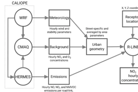
CALIOPE-Urban estimates hourly NO2 concentrations by coupling the CALIOPE mesoscale air quality forecasting system, providing background concentrations, meteorolog-ical data and road-link traffic emissions, with the R-LINE dispersion model adapted to street canyons. Here we intro-duce and describe the components of the coupled model as depicted in Fig. 1.
2.1 Mesoscale air quality forecasting system CALIOPE CALIOPE (Baldasano et al., 2011) integrates the Weather Research and Forecasting model version 3 (WRF; Ska-marock and Klemp, 2008), the High-Elective-Resolution Modelling Emission System (HERMES v2.0; Guevara et al., 2013), the Community Multiscale Air Quality Modeling System version 5.0.2 (CMAQ; Byun and Schere, 2006) and the mineral Dust REgional Atmospheric Model (BSC-DREAM8b; Basart et al., 2012). The mesoscale system is run over Europe at a 12 km×12 km horizontal resolution, Iberian Peninsula at 4 km×4 km and the Catalonian domain,
includ-Figure 1.CALIOPE-Urban workflow. Models are represented by circles and data by rectangular shapes. CALIOPE is left untouched. Meteorology and background from WRF and CMAQ are combined with urban geometry to create inputs for R-LINE. R-LINE dis-persion is left untouched, after adjusting meteorology and surface roughness for local urban geometry.
ing Barcelona, at 1 km×1 km. CALIOPE results have been evaluated in detail elsewhere (e.g. Pay et al., 2014).
In our system, WRF uses the Global Forecasting System (GFS) model initial/boundary conditions from the National Centers for Environmental Prediction (NCEP) to forecast the mesoscale meteorological conditions. Three nested domains are designed to provide a final high-resolution run over the Catalonian domain. In the vertical, WRF is configured with 38 sigma layers up to 50 hPa, where 11 cover the plane-tary boundary layer (PBL). Our WRF setup utilises the rapid radiation transfer model for long-wave radiation and Dud-hia for short-wave radiation, the Kain–Fritsch cumulus pa-rameterisation, the single-moment three-class microphysics scheme, the Yonsei University PBL scheme, and the Noah land-surface model based on the CORINE land-use data from the year 2006.
For the mesoscale model, pollutant emissions are obtained from the high-resolution emission model HERMES v2.0 gridded up to 1 km×1 km and temporal (1 h) resolution. HERMES v2.0 estimates atmospheric emissions for Europe and Spain according to the Selected Nomenclature for Air Pollution (SNAP) and taking the year 2009 as the reference period. Emissions are estimated for nitrogen oxides (NOx),
plants, industries), maritime (e.g. ports), air traffic (e.g. air-ports), agricultural machinery (e.g. tractors and harvesters) and road transport. For the rest of pollutant sources a com-bination of top-down approaches (i.e. residential/commercial combustion, energy consumption statistics combined with a population map) and downscaling methodologies (i.e. use of solvents, extraction and distribution of fossil fuels; specific spatial proxies and temporal profiles assigned to the Spanish National Emission Inventory by categories at third level of SNAP) is adopted. The results of the HERMES v2.0 model have been used to support several air quality evaluation and planning studies (e.g. Baldasano et al., 2014; Soret et al., 2014) as well as emission inventory intercomparison exer-cises (Guevara et al., 2017).
The chemical transport model used in the CALIOPE sys-tem is CMAQ v5.0.2. It uses the CB05 gas-phase chemical mechanism, the AERO5 aerosol scheme and an in-line pho-tolysis calculation. CMAQ vertical levels are collapsed from the 38 WRF levels to 15 layers up to 50 hPa with six lay-ers falling within the PBL. We use MOZART-4 as boundary conditions for the European domain.
2.2 Street-scale dispersion model: R-LINE
R-LINE is a near-road Gaussian dispersion model (Snyder et al., 2013) that incorporates state-of-the-art Gaussian dis-persion curves (Venkatram et al., 2013) to simulate disper-sion of road source emisdisper-sions. The model resolves either numerically or analytically the integration of the contribu-tions of point sources along a street segment (Snyder and Heist, 2013). The first option is more accurate and the lat-ter spends less time computing dispersion. The analytical version is best suited for near-ground-level sources and re-ceptors. In order to estimate NO2 concentrations, R-LINE incorporates a chemistry module to resolve simple NO to NO2 chemistry with the generic reaction set (GRS; Valen-cia et al., 2018) considering the chemical reactions in Ta-ble 1. The GRS chemistry mechanism solves the photochem-istry of NO2 assuming clear-sky conditions. Thus, it does not consider cloud effects on the NO2 photolysis rate, one of its major limitations. R-LINE has been applied to esti-mate exposure to traffic-related air pollutants in a large-scale study in Detroit, United States (Isakov et al., 2014). How-ever, to our knowledge it has not been applied to European cities, where street canyon morphology dominates. Hence, in order to apply R-LINE over Barcelona its meteorology has been adapted to street canyons as described in Sect. 2.3.1 and the background concentrations are obtained from the CMAQ model considering local meteorology and urban geometry as described in Sect. 2.3.3.
Table 1.Chemical reactions in the generic reaction set (GRS). ROC represents reactive organic compounds, RP represents radical pool, SGN represents stable gaseous nitrogen products and SNGN repre-sents stable non-gaseous nitrogen products.
ROC+hν→RP+ROC RP+NO→NO2 NO2+hν→NO+O3 NO+O3→NO2 RP+RP→RP RP+NO2→SGN RP+NO2→SNGN
2.3 Coupling CALIOPE with R-LINE
CALIOPE and R-LINE are coupled offline: first CALIOPE is run over Europe, the Iberian Peninsula and Catalonia and then R-LINE is executed for Barcelona city. This approach addresses two main challenges that have already been high-lighted in the research literature: (1) downscaling regional meteorology to the street scale to drive pollutant disper-sion and (2) obtaining background concentrations from the mesoscale model without double counting traffic emissions in regional- and street-scale models. In addition to these chal-lenges, we consider it relevant to couple meteorology and background concentrations in a consistent way, taking into account atmospheric stability and urban geometry when es-timating background contribution within urban streets. Here we describe our methodology when coupling the models to mitigate these challenges.
2.3.1 Meteorology
Most buildings in Barcelona have lower heights than the WRF bottom layer (40.6 m depth). WRF results are assumed to represent over-roof wind and stability conditions because its midpoint height (20.3 m) is similar to the average build-ing height (bh) in a typical neighbourhood of Barcelona (e.g. Eixample district, 20.7 m). WRF is executed consistently with the forecasting air quality system CALIOPE, giving a constant surface roughness (z0) equal to 1 m over the urban area. In order to apply R-LINE over Barcelona, its meteorol-ogy has been adapted to street canyons. We have developed a methodology to estimate specificz0based on urban geom-etry (e.g. building height, street width). Oncez0is adjusted, the displacement height (dispht), friction velocity (u∗), con-vective velocity scale (w∗), PBL height and Monin–Obukhov
length (L) are recalculated (Cimorelli et al., 2005). The in-crease inz0generally leads to a larger dispht,u∗,w∗and PBL height. Therefore,Lis less stable and atmospheric conditions are more convective. Ultimately, these adjustments have an effect on the way the winds are profiled and on the rate of dispersion of the roadway emissions within the urban area.
250 m×250 m (planar building density, bd; average build-ing height, bh; and buildbuild-ing height standard deviation, bhdev) and (2) specific aspect ratio (ar) for each street segment con-sisting of street-averaged building height divided by street width. The geometrical parameters are calculated from a Barcelona City Council dataset containing 2-D geometries and number of floors for each building (Barcelona City Council, 2016), assuming 3 m height for each floor.
To estimate specificz0for each street segment we propose a new morphometric method inspired by previous studies in the literature. z0 is composed by the WRF’s background roughness (z0bg) and the one estimated locally (Eq. 1), which incorporates building height influence through the range pa-rameter scaled by two parabolic ratios based on aspect ratio (arr) and building density (bdr). The range parameter (Eq. 2) andz0increase with bh following most morphometric meth-ods (e.g. Macdonald et al., 1998). In addition, range andz0 increase with an increasing bhdev. This assumption is based on Kent et al. (2017), who compared nine methods to es-timate z0, concluding that methods considering height vari-ability through bhdev (i.e. a higher bhdev brings an increase inz0) provide better results (e.g. Kanda et al., 2013). The pa-rameterC multiplying the equation for range calculation is an empirical constant set to 1/20 after calibrating the system with the NO2measurements used in this work for CALIOPE-Urban evaluation. The displacement height is calculated fol-lowing R-LINE methodology given a factor of displacement height (facdispht) equal to 5 (Eq. 3) as suggested by Snyder and Heist (2013).
z0=arr·bdr·range+z0bg (1)
range=C· bh+bhdev (2)
dispht=facdispht·z0 (3)
To model the influence of building density and aspect ra-tio, we use the findings of Oke (1988) based on wind tun-nel and experimental studies. Oke concluded that over-roof air roughness and satisfactory dispersion within the street canyon are maximum under similar geometrical conditions. Specifically, showing thatarequals 0.65 and bd equals 0.25 gives maximum roughness for overlying air and optimal dis-persion conditions in the street canyon.
In practice,z0increases with an increasingarto a maxi-mum ofar=0.65 and decreases forar>0.65 (Eq. 4). Addi-tionally, an increasing bd produces higher z0 until a max-imum at bd=0.25 and decreases for higher bd (Eq. 5). We model these ratios using parabolic shapes ranging from 0 to 1. Both urban characteristics are modelled using one parabola to the left of the maximum and another to the right due to the unsymmetrical distribution of the parameter val-ues within Barcelona city (see Fig. A1 in Appendix A). The parabolic ratios will be maximum (i.e. equal to 1) if the roughness effect is maximum. The ratios are prevented from
having negative values by setting a minimum of 0.
arr=
1.0−2.3·(ar−0.65)2 if ar is≤0.65
max 0,1.0−1.38·(ar−0.65)2 if ar is>0.65
(4)
bdr=
1.0−16.0·(bd−0.25)2 if bd is≤0.25
max 0,1.0−8.1·(bd−0.25)2 if bd is>0.25
(5)
In addition to thez0adjustment, we adjust the wind speed and direction to more closely represent the winds blowing down the street as constrained by the buildings, which is called “channelling” (similarly to Fisher et al., 2006). We have adapted R-LINE to incorporate the orientation of road-ways (and thus the buildings) where the wind direction fol-lows the street direction. This leads to a recalculation of the wind direction and speed for each roadway before emissions are dispersed within a city. Wind speed channelling is pa-rameterised following Soulhac et al. (2008), who showed that mean velocity along a canyon for any wind direction is directly proportional to the cosine of the angle between street direction and over-roof wind direction (i.e. angle of in-cidence).
wsch=wsbh·max(0.1,abs(cos(θ ))) , (6) where wschmeans channelled wind speed at roof level; the wind speed at roof level (wsbh) is taken from the WRF bot-tom layer in metres per second andθ is the angle of inci-dence. The minimum value of the right component is set to avoid an unrealistic zero value for wind speed. Its value of 0.1 is defined in line with Kastner-Klein et al. (2001), who showed that the minimum longitudinal mean flow ve-locity component at canyon top is equivalent to 0.12 times the above-canyon wind speed for perpendicular over-roof winds according to their wind tunnel experiments. Then, to estimate wind speed at street level a logarithmic profile in-corporated within R-LINE that is based on similarity theory (Monin and Obukhov, 1954) is used. In this work, we assume that recirculation flows within street canyons are negligible because R-LINE computes concentrations averaged over an hour, when recirculation and vehicle-induced turbulence are assumed to contribute to a well mixed, more homogeneous air mass driven by variable wind conditions. Additionally, evaluation of the potential impact of including recirculating flows across the canyon is not possible without multiple si-multaneous meteorological and pollutant measurements at a fine temporal scale, which are currently not available for Barcelona city.
2.3.2 Emissions
HERMES v2.0 provides hourly NOx and NMVOC road
Figure 2.NOx emissions in grammes per metre per hour in Barcelona city at 07:00 UTC on 11 April 2013 and location of the two fixed
monitoring stations used to estimate the NO2/NOxratio. White circles with letters inside represent the stations: tr is Eixample traffic station
and bg is Ciutadella Park urban background station.
by the R-LINE model algorithms to account for NO2 near-road chemistry (Valencia et al., 2018). Road transport emis-sions (i.e. exhaust, evaporative, wear and resuspension) are estimated combining the tier 3 method described in the EMEP/EEA air pollutant emission inventory guidebook (fully incorporated in version 5.1 of the COPERT IV soft-ware) with a digitised traffic network that contains specific information by road stretch for daily average traffic, mean speed circulation, temporal profiles and vehicular park pro-files. We note that HERMES v2.0 uses COPERT IV, which does not incorporate revised emission factors of NOxrelated
to the “dieselgate” scandal. Hence, NOxemissions from
traf-fic may be underestimated. Input activity data are obtained by combining different datasets, including traffic data from the Barcelona Automatic Traffic Counting Equipment and vehicle composition profiles derived from a remote-sensing campaign performed in different areas of Barcelona during 2010 (Barcelona City Council, 2010). In Barcelona, higher levels of traffic emissions are found in the city centre and in the highways surrounding the city (Fig. 2). In order to produce emissions in grammes per metre per second for straight street segments as required by R-LINE, we converted the digitised road network curved segments in HERMES to straight segments with no intermediate vertices using the
Douglas–Peucker algorithm in the QGIS simplify geometries tool (QGIS Development Team, 2017).
We have estimated the NO2/NOxratio following Carslaw
and Beevers (2004), which produces an approximation to the NO2primary contribution. This method relates total Ox
(NO2+O3) to total NOx(NO2+NO) at a traffic monitoring station subtracting Oxand NOxfrom a background site in
or-der to remove the effect of background and to only calculate the contribution at the traffic site. As the traffic station we used the Eixample site and as the urban background station we used Ciutadella Park (see Fig. 2), which is located up-wind of the dominant up-wind direction. Figure 3 compares Ox
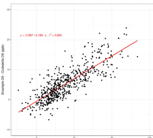
to NOxin Eixample after subtracting the background
repre-sented by Ciutadella from the beginning of October to end of February for the years 2012 to 2016. The photochemical season (April–September) is not used to avoid greater scatter than it is found in the winter months as shown by Clapp and Jenkin (2001). The Ox slope value of 18.9 % is considered
an estimate of the potential primary NO2contribution from vehicles at the Eixample traffic station. This value is consis-tent with studies conducted in other cities with a large diesel vehicle fleet (e.g. Carslaw et al., 2016; Wild et al., 2017) and is assumed to represent the NO2/NOxratio in Barcelona in
Figure 3.Scatter plot showing daylight mean Oxand NOxrelation
of the difference between Eixample and Ciutadella stations from the beginning of October to the end of February for the years 2012 to 2016.
2.3.3 Background concentrations
We use the upwind urban background scheme (UBS) to avoid the double counting of traffic emissions when coupling the mesoscale with the street-scale model. The UBS makes a se-lective choice of CMAQ cells as sketched in Fig. 4 to esti-mate over roof background concentrations. For each hour, a polygon covering upwind air masses (white) is created. In the figure, the average distance traversed by air masses dur-ing an hour (10.8 km) is estimated for WRF’s bottom layer wind speed (3 m s−1 in the image). Squares falling within the scheme polygon represent CMAQ cells and their colour refers to cell pollutant values (e.g. NO2at peak traffic hours may be higher within the city than over the Mediterranean Sea). Grid cell values falling over the scheme polygon are inverse-distance averaged to produce the background esti-mate of the scheme. Under calm conditions, only the upwind cell is chosen. This method is inspired by Berkowicz (2000), who apply a similar concept based on air mass trajectory to develop a background model.
Background concentrations are required at each receptor in CALIOPE-Urban. Urban dispersion models are typically run at a very high spatial resolution (e.g. 20 m×20 m). Run-ning the UBS every 20 m would have a high computational cost due to its spatial computations, and background concen-tration values are not expected to vary substantially over tens of metres because CMAQ produces results with 1 km×1 km spatial resolution. Hence, we first run the UBS to produce background concentration values at CMAQ grid cell
cen-Figure 4.Upwind urban background scheme concept. Basemap source: Esri (2019).
troids; then we apply a bilinear interpolation method to pro-vide background at very high spatial resolution.
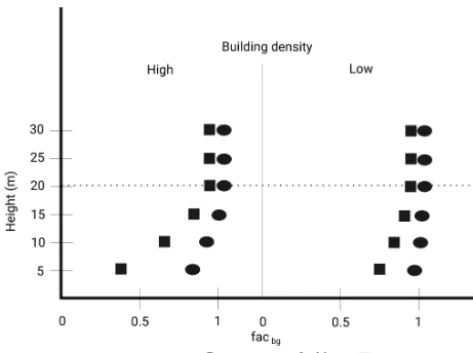
In addition to the UBS we implement a background de-cay method to calculate the surface level background con-centrations assuming that the UBS provides the concentra-tion at rooftop level. To calculate street level NO2 concen-trations, the vertical distribution of pollutants is solved first using the background decay method, applied uniformly to all pollutants, and then the GRS chemical mechanism is solved. The relationship between rooftop and surface level concen-trations is assumed to depend on atmospheric stability, lo-calised surface roughness and urban geometry (see Fig. 5 as an illustration of the background decay concept). In the research literature, the influence of atmospheric stability on vertical mixing within a street canyon has been demonstrated using experimental measurements (Rotach, 1995) and wind tunnel experiments (Salizzoni et al., 2009), and it has been implemented in some dispersion models (e.g. Soulhac et al., 2011; Kim et al., 2018). The ratio of wind speeds at surface and rooftop levels (wssfc/wsbh) estimated by R-LINE using similarity theory (Monin and Obukhov, 1954) is used as a proxy for the vertical mixing. Using this ratio, we calculate facbg that represents the adimensional vertical mixing vari-able that is multiplied to rooftop background concentration to obtain surface level background concentration at a given height. Wind channelling does not affect the ratio wssfc/wsbh because we assume that channelling equally affects winds at surface and rooftop levels.
Figure 5. Illustration of the background decay method concept. Building height is approximately 20 m.
convective conditions for values higher than 0.30. This value is set to exclude slightly stable night hours with low posi-tive hflux values mainly caused by the urban heat island (i.e. Barcelona city has been found to be 2.9◦C warmer than its periphery by Moreno-Garcia, 1994). The following parame-terisation is used for cases with bd higher than 0.1,
facbg=
1−F+wssfc/wsbh·F if hflux is>0.30 wssfc/wsbh if hflux is≤0.30, (7) whereF =m+abs(0.25−bd), withmbeing an empirical parameter set to 0.35 after system calibration with NO2 mea-surements; hflux is upward heat flux at the surface (W m−2). Surface background concentrations for convective situations are maximum for bd equal to 0.25 consistent with thez0 es-timation in Sect. 2.3.1. Conversely, we assume that for bd close to zero, surface background concentrations tend lin-early to rooftop level background concentrations. The thresh-old bd=0.1 is based on Grimmond and Oke (1999), who set it as an inferior limit for real cities and show that below this value an isolated flow regime governs. Within this regime, street level and over-roof air is well mixed due to the low building density. Hence, for cases with bd equal to or lower than 0.1, facbgtends linearly to 1 following
facbg=
1−5·bd+wssfc/wsbh·(5·bd) if hflux is>0.30
1−10·bd+wssfc/wsbh·(10·bd) if hflux is≤0.30
. (8)
Equation (8) shows linear variations between the point at bd=0 and facbg=1 and the point at bd=0.1 with the corre-sponding facbgvalue from Eq. (7).
2.4 Execution setup
We have run CALIOPE-Urban for receptors as far as 250 m from roads with sufficient annual average daily traffic
(AADT) (i.e. 2000 vehicles per day following Jensen et al., 2017) and receptors further away directly receive CMAQ val-ues interpolated. The 250 m limit is chosen as similar but less restrictive (i.e. to allow longer distances under stable hours) than the one used in Beevers et al. (2012), who used 225 m for London. To smooth out the variation between system out-puts, we define a transition area (i.e. 140 to 250 m) where re-ceptors are given concentration values weighted by distance. For temporal and spatial evaluation runs, we locate receptors at the specific coordinates of the measurement sites.
To obtain high-resolution concentration maps for the en-tire city, we set the spatial context as the minimum rectangle where Barcelona municipality is contained and extended it by 250 m buffers that include the highways surrounding the city. The context is covered by a regular receptor grid of 10 m resolution. R-LINE execution loops over each hour, road and receptor to estimate the contribution from each source to each receptor.
Aiming to understand the impact on accuracy of the lo-cal parameterisation for background and meteorology and the impact of using the analytical approach for dispersion, we have run CALIOPE-Urban with different configurations. In Table 2, we describe the different scenarios that have been run. As seen in the table, the CALIOPE-Urban and the CALIOPE-Urban analytical configurations make use of the developed local parameterisations for background and me-teorology. In contrast, the CALIOPE-Urban-nl (non-local) configuration does not apply the local parameterisations for background and meteorology. Instead, it uses as background the UBS output without vertical mixing and it omits the use of wind channelling and specific stability parameters for each street segment based on localz0. We show this configura-tion’s results in order to understand if the new implementa-tions in this work contribute substantially to improve the sys-tem’s ability to simulate NO2concentrations in Barcelona. R-LINE dispersion algorithm options (i.e. analytical and nu-merical) are described in Sect. 2.2. For meteorological op-tions, we refer to Sect. 2.3.1. The background method is de-scribed in Sect. 2.3.3.
3 Observational datasets
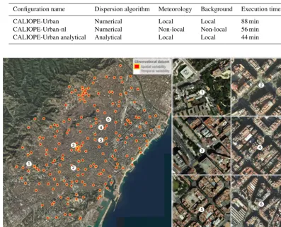
We use three datasets of observations to evaluate the perfor-mance of CALIOPE-Urban to reproduce the temporal and spatial variation in NO2 concentrations within Barcelona city. Figure 6 shows the locations of measurements used in this study, which are described below.
3.1 NO2temporal variability: street canyon campaign
and permanent XVPCA network
Table 2.Description of the execution setup. Execution time is for the entire city of Barcelona during 1 h running CALIOPE-Urban (i.e. only the urban system, after CALIOPE run completion) over 11 251 street segments and 965 458 receptors at 10 m×10 m spatial resolution.
Configuration name Dispersion algorithm Meteorology Background Execution time
CALIOPE-Urban Numerical Local Local 88 min CALIOPE-Urban-nl Numerical Non-local Non-local 56 min CALIOPE-Urban analytical Analytical Local Local 44 min
Figure 6.Passive dosimeter and monitoring site locations used in the evaluation of CALIOPE-Urban in this work. Red dots with a yellow border represent passive dosimeters (spatial performance) and white numbered dots depict monitoring site emplacements (temporal variabil-ity). White dots numbered 1 (Palau Reial), 2 (Eixample) and 3 (Gràcia-Sant Gervasi) are air quality monitoring sites and 4 (213 Industria Street), 5 (445 Valencia Street) and 6 (309 Industria Street) correspond to mobile units. Basemap source: Esri (2019).
conducted using mobile units in April and May 2013 in Barcelona (Amato et al., 2014). The official monitoring net-work has 10 stations in Barcelona and only two of them (i.e. Gràcia-Sant Gervasi and Eixample) are considered represen-tative of near-traffic conditions and provide NO2hourly lev-els. Measured data from three sites of the official network are used in this study: Eixample and Gràcia-Sant Gervasi (traf-fic) and Palau Reial (background). Both traffic sites are lo-cated in complex wide areas where several streets intersect (see sites 2 and 3 in Fig. 6 and in the description of Ta-ble 3). Palau Reial station (i.e. site 1 in Fig. 6) is located in a medium bd area of the city, 300 m away from a heavily trafficked street. This dataset is complemented with obser-vations from an experimental campaign where mobile units placed at the parking lane of several street segments mea-sured air quality parameters at 3 m height. For this study, we used data gathered every 30 min and aggregated to hourly levels for homogeneity at 213 Industria Street, 309 Indus-tria Street and 445 Valencia Street. These streets present a
marked canyon pattern (see sites 4, 5 and 6 in Fig. 6 and de-scription Table 3) where the aspect ratio is approximately 1. In Barcelona, different street geometrical patterns cohabit. For example, the Eixample district, which has the high-est number of inhabitants and the greathigh-est population den-sity (33 000 inhabitants km−2), is characterised by a marked street canyon pattern. Most of its canyons are about 20 to 25 m high and 20 m wide (i.e.ar=1 and higher than 1). Ex-perimental campaign sites are considered traffic sites in this work because they are exposed to similar AADT and traf-fic density (td) compared to oftraf-ficial traftraf-fic sites as shown in Table 3. We apply Eq. (9) to obtain td over an area of 1 km2.
td=
n
X
s=1
tfs·ls, (9)
measurement site,ls represents the length of the street seg-mentsin metres and tf represents the traffic flow passing a transverse section of the street segmentsexpressed in vehi-cles per second. To obtain tf, AADT is divided by 3600·24 and multiplied by a temporal factor (i.e. 1.47) representing a typical factor for the morning traffic peak in Barcelona. 3.2 NO2spatial variability: passive dosimeter
campaign across the city
With the objective of representing the NO2spatial variabil-ity, 212 passive dosimeters were located in Barcelona from 28 February to 15 March 2017 as depicted by red dots with a yellow border in Fig. 6. In every square kilometre of surface there were at least two dosimeters, representing the back-ground and traffic conditions at 2.2–2.5 m height. The 100 background dosimeters were placed more than 10 m away from the road and the 112 traffic dosimeters were located less than 3 m away from the road and at least 25 m away from intersections. To ensure the equivalence of measurements to standard conditions, these were corrected through com-parison with reference equipment from several sites of the XVPQA network. After a preliminary inspection of the loca-tion of the dosimeters, we discarded data from 30 dosimeters to avoid results that could not be interpreted for several rea-sons (e.g. dosimeter and simulated road at different heights, highway covered by a tunnel near dosimeter location that is not considered in the emission inventory, lack of emission sources near dosimeter).
4 Results and discussion
Section 4.1 presents the temporal variability of NO2 concen-trations estimated by CALIOPE and CALIOPE-Urban com-pared to observations at the six sites described in Sect. 3.1. Section 4.2 describes the results in terms of the spatial vari-ation during the 2-week passive dosimeter campaign de-scribed in Sect. 3.2. Model performance is quantified using performance measures as described by Chang and Hanna (2004) and using assessment target plots (defined in the FAIRMODE initiative; Janssen et al., 2017). The perfor-mance statistics used here are the geometric mean bias (Ge-oMean), the fraction of model results within a factor of 2 of observations (FAC2), the geometric standard deviation (GeoSD), the correlation coefficient (R), the mean bias (MB) and the root-mean-square error (RMSE). The mathemati-cal expressions of these statistics can be found in the Ap-pendix C.
4.1 Temporal variation in NO2concentrations within
urban streets
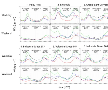
The scatter plots of Fig. 7 compare CALIOPE and CALIOPE-Urban outputs with observations based on hourly, daily mean and maximum modelled concentrations at the six
sites described in Sect. 3.1 for April and May 2013. In gen-eral, CALIOPE-Urban shows a greater agreement for hourly, daily means and maximum concentrations but tends to under-predict daily peak concentrations at sites not exposed to very high traffic intensity (i.e. sites where urban background con-tribution predominates like Gràcia-Sant Gervasi). During the study period most daily maxima (i.e. 56 %) occur at morn-ing or evenmorn-ing traffic peak times (i.e. 06:00–07:00 or 18:00– 20:00 UTC) when atmospheric conditions are typically sta-ble and traffic intensity is high.
Table 4 shows the model performance statistics com-puted with hourly data, including the CALIOPE-Urban-nl run. We compare CALIOPE-Urban and CALIOPE-Urban-nl to assess the difference in performance derived by the use of the local developments described in Sect. 2.3. All systems perform well at urban background sites and only CALIOPE-Urban gives good agreement with observations in traffic sites. The greatest difference between CALIOPE and CALIOPE-Urban system performance is produced at the 445 Valencia Street site due to its street canyon morphology (ar=0.86). At this site, the mean transport is well resolved by the channelled winds, and its high AADT produces a high increase in traffic emissions within R-LINE. CALIOPE-Urban-nl largely overestimates NO2 concentrations at this site for several reasons: it directly uses the output of UBS for background, instead of applying the vertical mixing that re-duces background at street level especially under stable con-ditions;z0is given the WRF value (z0=1.0), which is much lower than its locally estimated value (i.e.z0=2.2; see Ta-ble 3), that enhances dispersion decreasing concentration lev-els; lastly pollutant dispersion is not channelled within the street, so higher contributions of nearby streets may be ex-pected.
Table 3.Morphometric and traffic description of measurement sites used in CALIOPE-Urban evaluation. The measurement height of the official network sites and the mobile sites is 3 m. AADT from the nearest street is considered. The traffic density (td) is estimated following Eq. (9). The Palau Reial td is not included because it is an urban background site not directly exposed to high traffic.
Site ar bh bd bhdev z0 AADT td
(m) (m) (m) (vehicles d−1) (vehicles km−2s−1)
1. Palau Reial 0.12 14.6 0.12 6.4 1.27 3900 – 2. Eixample 0.00 21.1 0.40 8.4 1.03 41 000 5666 3. Gràcia-Sant Gervasi 0.38 17.2 0.45 7.1 1.68 12 700 3884 4. 213 Industria Street 1.00 18.1 0.38 8.3 1.94 15 200 3003 5. 445 Valencia Street 0.86 19.5 0.32 7.2 2.20 32 500 5978 6. 309 Industria Street 1.03 17.0 0.31 8.1 1.97 12 900 3320
Table 4.NO2model evaluation statistics calculated at six sites (described in Sect. 3) for hourly concentrations during April and May 2013 for CALIOPE, CALIOPE-Urban and CALIOPE-Urban without local developments (CALIOPE-Urban-nl). Bold numbers represent model results with better performance for each statistic and site.
Site Method FAC2 MB RMSE GeoMean GeoSD r
1. Palau Reial CALIOPE 0.73 −1.23 24.11 1.10 1.25 0.55 CALIOPE-Urban 0.72 −8.70 21.57 1.28 1.22 0.57 CALIOPE-Urban-nl 0.67 3.61 26.34 1.28 1.22 0.55
2. Eixample CALIOPE 0.60 −8.57 35.14 1.35 1.35 0.34 CALIOPE-Urban 0.86 9.38 26.70 0.83 1.11 0.55 CALIOPE-Urban-nl 0.61 39.53 54.92 0.57 1.38 0.45
3. Gràcia-Sant Gervasi CALIOPE 0.55 −10.95 31.95 1.38 1.39 0.47 CALIOPE-Urban 0.79 −7.39 25.11 1.07 1.19 0.52 CALIOPE-Urban-nl 0.66 6.00 35.91 0.91 1.43 0.38
4. 213 Industria Street CALIOPE 0.52 −19.13 35.13 1.79 1.54 0.44 CALIOPE-Urban 0.78 −13.62 26.55 1.30 1.17 0.57 CALIOPE-Urban-nl 0.75 1.57 31.12 1.04 1.26 0.54
5. 445 Valencia Street CALIOPE 0.50 −21.94 38.31 1.85 1.53 0.43 CALIOPE-Urban 0.92 2.92 23.26 0.94 1.07 0.56 CALIOPE-Urban-nl 0.79 23.72 42.29 0.75 1.19 0.47
6. 309 Industria Street CALIOPE 0.64 −7.41 28.49 1.36 1.33 0.53 CALIOPE-Urban 0.84 −4.60 22.72 1.05 1.13 0.53 CALIOPE-Urban-nl 0.78 11.60 31.13 0.83 1.24 0.58
spends approximately half the time computing in comparison to the numerical dispersion algorithm as shown in Table 2.
Figure 8 shows NO2assessment target plots for CALIOPE and CALIOPE-Urban. In the plots the centred root-mean-square error (CRMSE) for each measurement station is plot-ted against the normalised bias. Distance from circle origin gives an estimate for the model quality indicator (MQI; Thu-nis and Cuvelier, 2016) that measures general model accu-racy depending on measurement uncertainty. MQI values be-low 1 (i.e. green shading area) are considered to comply with the model quality objective. All sites in the CALIOPE-Urban simulation fall within the green shaded area (i.e. comply-ing with FAIRMODE’s model quality objective). In contrast, four out of six in CALIOPE lie within the green shaded area,
clearly showing the positive effect of the street-scale model in the coupled system.
Figure 7.Scatter plot of hourly(a, b), daily mean(c, d)and daily maximum(e, f)modelled concentrations against observed concentrations with colours representing monitoring sites for CALIOPE(a, c, e)and CALIOPE-Urban(b, d, f). Purple represents Palau Reial, the urban background site. The other colours represent traffic sites as described in Sect. 3.1.
may bring CALIOPE-Urban to generally overestimate for those hours as found in the literature near road sites (Hood et al., 2018). However, the vertical mixing implemented in CALIOPE-Urban decreases background concentration mix-ing from aloft durmix-ing night hours because under stable at-mospheric conditions vertical mixing is reduced compared to daylight hours, which are more convective. This effect can be noticed in the difference between CALIOPE-Urban and CALIOPE-Urban-nl from 00:00 to 06:00 and from 18:00 to 23:00 (UTC) at traffic sites (i.e. sites 2, 3, 4, 5 and 6 in Fig. 9), where CALIOPE-Urban concentration levels correct the night overestimations seen in CALIOPE-Urban-nl. Such
a result shows the benefit of considering the vertical stability in the coupling procedure of the mesoscale and the street-scale dispersion model.
Figure 8.NO2model assessment target plots for CALIOPE (left) and CALIOPE-Urban (right). Symbols correspond to the six measurement sites described in Sect. 3.1 and the MQI for each site is represented by the distance between the circle origin and the site symbol.
traffic at 213 Industria Street site could bring a model accu-racy improvement. However, the lack of observational traffic count data at the monitoring sites does not permit us to ex-plore the precision of the input AADT information consid-ered in HERMES v2.0 at those locations.
4.2 Spatial variation in NO2concentrations across the
city
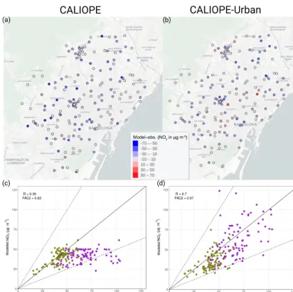
We evaluate CALIOPE and CALIOPE-Urban NO2in terms of spatial variations across Barcelona city using measure-ments from 182 valid passive dosimeters as described in Sect. 3.2. Table 5 gives statistics at the 182 sites where passive dosimeters measured NO2 concentrations for a 2-week period (28 February–15 March 2017) for CALIOPE, CALIOPE-Urban and CALIOPE-Urban-nl (without local developments).
Considering all sites, CALIOPE-Urban shows a much bet-ter correlation coefficient (0.70 vs. 0.36) than CALIOPE due to its good performance at traffic sites. Compared to CALIOPE-Urban-nl their correlation is similar. If we con-sider only urban background sites, CALIOPE shows a greater correlation coefficient than CALIOPE-Urban (0.66 vs. 0.54) and a MB closer to 0. In addition, CALIOPE-Urban-nl gives a better correlation than both systems. A potential expla-nation for this result is related to the error compensation shown in the temporal evaluation (Sect. 4.1). CALIOPE and CALIOPE-Urban-nl may compensate for the underestima-tion during daytime with the overestimaunderestima-tion during night-time. In contrast, CALIOPE-Urban may not compensate for the daytime underestimations with overestimated night val-ues because the background is reduced due to low verti-cal mixing effect during night-time (stable) hours. An en-hanced daytime NO2 background contribution would im-prove CALIOPE-Urban accuracy at urban background sites. For traffic sites, CALIOPE shows a strong underestima-tion (MB= −25.57 µg m−3) and CALIOPE-Urban gives MB levels closer to 0. CALIOPE-Urban underestimations may be influenced by afternoon underestimations and a misrepresen-tation of traffic emissions in some areas of the city. In con-trast, CALIOPE-Urban-nl gives a high MB and the highest RMSE among the three systems. This tendency to overesti-mate near traffic of CALIOPE-Urban-nl may be due to the reasons stated in Sect. 4.1. In general, closer to intense traf-fic CALIOPE-Urban is very sensitive to emissions and its dispersion characterises the spatial variability for the study period well. Reproducing spatial gradients near intense traf-fic is crucial in a city like Barcelona given its high vehicle density and NO2concentration levels.
Figure 10 shows the difference between CALIOPE and CALIOPE-Urban results and measurements (panels a, b) and scatter plots at all sites (panels c, d) distinguished with colours by site type (e.g. traffic site, urban background site). In Fig. 10a the concentration difference map of CALIOPE shows an overall underestimation, represented by blue dots.
This underestimation is found to be systematic at traffic sites in the scatter of Fig. 10c (purple dots), where modelled val-ues barely exceed 50 µg m−3 while most of the observed values at traffic sites are above that value. In contrast, the CALIOPE-Urban difference map (Fig. 10b) shows a more mixed picture with a broader representation of white dots (bias close to 0) but also more red ones in the city centre and close to the highways. For CALIOPE-Urban’s scatter, most of the model results at traffic sites are within the 1:2 and 1:0.5 dashed lines, showing a better agreement at traffic sites than CALIOPE (Fig. 10d). In CALIOPE-Urban’s dif-ference map, we see a spatial pattern with average bias close to 0 in the city centre, where traffic is denser and close to the highways surrounding the city. The appearance of red dots may indicate that CALIOPE-Urban overestimates close to high trafficked areas while CALIOPE underestimates in these areas. This may be due to an overestimation of traf-fic emissions or background concentrations in these areas. In contrast, in locations where traffic is not very intense (see Fig. 2 for NOx emissions) CALIOPE-Urban shows
system-atic underestimations. This result may be derived from the systematic underestimation of midday NO2 concentrations in low-traffic areas as shown in Sect. 4.1.
4.3 Major uncertainty sources
Here we discuss potential sources of error in our model by analysing episodes when the model was skilful compared with episodes when the model was not. Our analysis solely considers the meteorological and background concentration inputs as potential sources of error. While road traffic emis-sion estimates may introduce large errors, we lack observa-tions of traffic counts at the measurement site locaobserva-tions to properly assess them.
We calculated daily the RMSE of the hourly modelled NO2 concentrations versus the observed values at the six sites described in Sect. 3.1 during the period April and May 2013. For each site we picked the 10 d with the highest RMSE and 10 d with the lowest RMSE as potential candi-dates. Then, we put together the candidates of all sites and we chose the most frequent 5 d (i.e. from good and bad perfor-mance candidate days) for both CALIOPE and CALIOPE-Urban, finding that both systems share to a large extent the days with skill (four out of five days) and without (three out of five). This result shows that the coupled system mance is highly dependent on the mesoscale model perfor-mance. To explore errors potentially caused by R-LINE in-puts, in Fig. 11 we compare the five days with less skill (i.e. 11, 16, 17 April and 7, 8 May) and the five days with more skill (i.e. 7, 20 April and 18, 19, 25 May) with observations for wind speed (ws), street level NO2and background NO2.
Table 5. NO2 model evaluation statistics calculated at 182 passive dosimeter valid sites (described in Sect. 3.2) during 2 weeks from 28 February to 15 March 2017 for CALIOPE, CALIOPE-Urban and CALIOPE-Urban-nl mean concentrations. Bold numbers represent model results with better performance for each statistic and site. Results are shown for all (including traffic and urban background), only urban background and only traffic sites.
Sites Method FAC2 MB RMSE GeoMean GeoSD r
All CALIOPE 0.92 −14.00 21.88 1.30 1.08 0.36 CALIOPE-Urban 0.97 −7.26 17.21 1.20 1.06 0.70 CALIOPE-Urban-nl 0.98 15.24 28.30 0.81 1.06 0.69
Background CALIOPE 1.00 −2.84 8.08 1.06 1.02 0.66 CALIOPE-Urban 0.97 −7.34 12.71 1.23 1.06 0.54 CALIOPE-Urban-nl 1.00 10.09 15.03 0.82 1.04 0.72
Traffic CALIOPE 0.81 −25.57 30.74 1.60 1.63 0.22 CALIOPE-Urban 0.97 −7.17 20.62 1.17 1.06 0.53 CALIOPE-Urban-nl 0.96 20.17 36.76 0.81 1.08 0.50
underestimated under calm conditions (Fig. 11d), other pro-cesses (e.g. atmospheric stability) may have a greater impor-tance in this case. In our coupling under very stable atmo-spheric situations, dispersion is reduced and background in-jection from the overlying atmosphere is limited. This control mechanism adapts the system to specific street conditions, regulating dispersion and background injection. For these days, an extended observational dataset would be needed to better understand the model behaviour.
To analyse the background concentrations from the mesoscale simulation as a potential error source, we com-pared NO2 observations from the Ciutadella urban back-ground station with hourly modelled concentrations averaged over the six sites. We aimed to compare the modelled back-ground concentrations (i.e. excluding local vehicular traffic contribution) with the most representative urban background observation, which in our case is the Ciutadella site. The results shown in Fig. 11e, f represent concentrations pro-vided by upwind CMAQ grid cells depending on wind speed and direction (blue) as described in Sect. 2.3.3 downscaled to surface level using the vertical decay method (green). As expected, observed NO2 concentrations on days with calm conditions and therefore poor skill are higher than on those with enhanced ventilation and better skills. The back-ground model reproduces the variation during both types of days well but overestimates concentrations during night-time (19:00–22:00 UTC), particularly during days with calm con-ditions. This problem is partially corrected by using the back-ground vertical decay method as seen in Fig. 11f and in Fig. 9. In addition, NO2 concentrations are underestimated at the beginning of the day (01:00–04:00 UTC). The fact that the averaged diurnal cycle in Fig. 9 shows similar error pat-terns suggests that NO2 background concentrations greatly influence NO2street level concentrations in agreement with Degraeuwe et al. (2017).
4.4 Hourly variation in street NO2concentrations
Hourly street NO2 concentrations are expected to vary spa-tially and temporally with higher values close to intense traf-fic sites during rush hour. Figure 12 shows high-resolution (10 m×10 m) NO2concentration maps at four different hours on Thursday 11 April 2013 (i.e. 00:00, 07:00, 12:00 and 18:00 UTC). This day is chosen because it shows a marked diurnal cycle with maxima consistent with the morning and evening traffic peaks (i.e. 06:00–07:00 or 18:00–20:00 UTC). Higher concentrations are found at 07:00 and 18:00 UTC where high traffic emissions are concentrated (i.e. highways surrounding the city and city centre) because traffic intensity is higher at these hours of the day and the atmosphere tends to be stable, making pollutant dispersion more difficult. Con-versely, lower concentrations are found at 00:00 UTC due to the lower traffic intensity and at 12:00 UTC. At 12:00 UTC traffic intensity is considerably higher than at 00:00 UTC but the atmosphere is more convective and pollutant dispersion is enhanced.
Figure 10. (a, b)NO2concentration difference (model – observations) for 2-week averaged values during the dosimeter campaign in 2017; CALIOPE is left(a)and CALIOPE-Urban is right(b).(c, d)Scatter plot of modelled vs. observed concentrations with colours representing site type (olive green for background and purple for traffic) for CALIOPE(c)and CALIOPE-Urban(d). Correlation (R) and agreement factor of 2 (FAC2) are computed for all sites.
5 Conclusions
This study describes the development of a coupled regional-to street-scale modelling system, CALIOPE-Urban, which provides high-spatial- and high-temporal-resolution (up to 10 m×10 m, hourly) NO2 concentrations for Barcelona. It couples the mesoscale air quality forecasting system CALIOPE (WRF-HERMES-CMAQ-BSC-DREAM8b) with the urban roadway dispersion model, R-LINE. For each re-gional 1 km×1 km grid cell, meteorological data from WRF and background concentrations from CMAQ are used as input combined with traffic emissions from the HERMES emission model at road link level. R-LINE has been adapted to Barcelona’s geometrical conditions by considering
spe-cific meteorology and background concentrations for each street. CALIOPE-Urban NO2simulations are compared with CALIOPE and with observations for temporal evaluation, us-ing data from five traffic sites and one urban background site during April and May 2013, and for spatial evaluation, with NO2concentrations measured by 182 passive dosimeters dis-tributed across the entire city during 2 weeks in February-March 2017.
Figure 11.Box plots by time of the day of good(a, c, e)and bad performance days(b, d, f)for CALIOPE-Urban inputs and observations with dots representing outliers. Panels(a, b)represent WRF and observed wind speeds at Barcelona airport (10 m height); panels(c, d)show observed and modelled NO2concentrations for the six sites in Sect. 3.1; panels(e, f)depict NO2observed concentrations at the Ciutadella urban background station and background model averaged results at the six sites. Observed values are orange and modelled results are blue. Light green represents background model results at the surface level.
street. Regarding background concentrations, it estimates over-roof levels using an upwind background scheme and gives surface concentrations by applying a vertical mixing parameterisation based on urban geometry and atmospheric stability. The upwind background scheme avoids double
Figure 12.NO2high-resolution (10 m×10 m) concentration maps on 11 April 2013. The resolution is for the entire concentration map. Panel (a)represents concentrations at 00:00 UTC (2:00 LT),(b)07:00 UTC (9:00 LT),(c)12:00 UTC (14:00 LT) and(d)18:00 UTC (20:00 LT). Basemap source: Esri (2019).
background concentrations at surface level, the vertical mix-ing parameterisation enhances background mixmix-ing from the overlying atmosphere under daytime convective atmospheric conditions and limits background air mixing during night-time (stable) hours. For the transition from urban to subur-ban areas, CALIOPE-Ursubur-ban implements a smooth variation for wind conditions, background and total concentrations.
Temporally, CALIOPE-Urban agrees better with observa-tions than CALIOPE at the five traffic sites evaluated, where the contribution of local emissions predominates. For the ur-ban background site of Palau Reial, both systems give simi-lar (good) results. For traffic sites, the coupled system shows better agreement in highly trafficked areas where local dis-persion plays a crucial role. Regarding the diurnal average cycle at the observation sites, both systems follow the over-all daily cycle in the observations but CALIOPE-Urban pre-dicts better morning peaks, and corrects the afternoon levels at traffic sites as well as the systematic night-time
overesti-mation produced by the regional system. The vertical mix-ing of rooftop background concentrations to surface levels based on atmospheric stability and urban geometry appears to be a good method to correct the strong positive bias of the mesoscale model under stable atmospheric conditions during the evening.
area, the better CALIOPE-Urban performance is compared to the regional system.
When exploring the main error sources, overall both sys-tems produce results that are either accurate or inaccurate on the same days. This fact suggests that coupled system results are highly influenced by the regional system results. Fur-thermore, we find that CALIOPE-Urban gives higher errors (i.e. stronger underestimations) under stable conditions with light winds and low PBL height than under more convec-tive conditions, with stronger winds and higher PBL heights. Another potential source of uncertainty is the integration within HERMES v2.0 of COPERT IV instead of COPERT V, which considers diesel NOx exceedances derived from
the dieselgate scandal for EURO 5 and EURO 6 diesel cars (Brown et al., 2018). In future work, we plan to update HER-MES v2.0 with the new emission factors released by COP-ERT V and examine the influence of traffic emissions in CALIOPE-Urban results. Finally, we consider an additional source of uncertainty, the assumption of clear-sky conditions in the photolysis rate calculation of the GRS chemistry mech-anism.
For high-resolution air quality forecasts, we show that CALIOPE-Urban using either the numerical or the analyti-cal dispersion algorithm gives good results. However, an en-tire city system execution using the analytical configuration takes approximately half the time compared to the numeri-cal one. Hence, the analytinumeri-cal dispersion algorithm may be a suitable option for forecasting applications when sources, such as roadways, and receptors are located near the ground. We show that traffic monitoring stations in Barcelona do not represent the highest NO2concentrations in the city. We find the highest levels in heavily trafficked street canyons that are not well ventilated and near highways in the city sur-roundings. As a consequence, we consider that additional monitoring sites located in these areas may better charac-terise the range of NO2concentration levels in Barcelona and give a better representation of human exposures.
This study has demonstrated that CALIOPE-Urban im-proves the accuracy of model outputs estimating NO2 concentrations in Barcelona compared to CALIOPE. The methodology is replicable in cities where a mesoscale chem-istry transport model provides NO2simulations if urban ge-ometrical data are available. The next step is to implement CALIOPE-Urban in the operational forecasting system for Barcelona to provide NO2concentrations at street level, and explore emission impacts due to improved NOxemission
es-timates.
Appendix A: Extended urban geometry characterisation
Appendix B: Extended performance evaluation
Table B1.NO2model evaluation statistics calculated at six sites (described in Sect. 3) during April and May 2013 for CALIOPE and CALIOPE-Urban daily mean concentrations. Bold numbers represent model results with better performance for each statistic and site.
Site Method FAC2 MB RMSE GeoMean GeoSD r
1. Palau Reial CALIOPE 1.00 −10.97 15.44 1.30 1.08 0.84 CALIOPE-Urban 0.95 −8.72 13.85 1.29 1.07 0.80
2. Eixample CALIOPE 0.91 −9.62 17.37 1.24 1.08 0.52 CALIOPE-Urban 1.00 9.64 15.60 0.83 1.04 0.60
3. Gràcia-Sant Gervasi CALIOPE 0.91 −10.97 15.44 1.30 1.08 0.82 CALIOPE-Urban 1.00 −7.40 15.33 1.10 1.05 0.81
4. 213 Industria Street CALIOPE 0.75 −19.15 23.51 1.62 1.20 0.68 CALIOPE-Urban 0.95 −13.79 18.90 1.29 1.07 0.68
5. 445 Valencia Street CALIOPE 0.70 −22.05 26.07 1.64 1.20 0.67 CALIOPE-Urban 1.00 3.00 11.25 0.94 1.02 0.65
6. 309 Industria Street CALIOPE 0.95 −7.13 13.33 1.22 1.07 0.78 CALIOPE-Urban 0.95 −7.12 13.32 1.30 1.07 0.68
Table B2.NO2model evaluation statistics calculated at six sites (described in Sect. 3) during April and May 2013 for hourly concentrations of CALIOPE-Urban, CALIOPE-Urban analytical or CALIOPE-Urban-nl (non-local) configurations. Bold numbers represent model results with better performance for each statistic and site.
Site Method FAC2 MB RMSE GeoMean GeoSD r
1. Palau Reial CALIOPE-Urban 0.72 −8.70 21.57 1.28 1.22 0.57 CALIOPE-Urban analytical 0.69 −10.46 22.44 1.38 1.24 0.56 CALIOPE-Urban-nl 0.67 3.61 26.34 0.99 1.40 0.55
2. Eixample CALIOPE-Urban 0.86 9.38 26.70 0.83 1.12 0.55 CALIOPE-Urban analytical 0.87 7.99 26.25 0.85 1.11 0.56 CALIOPE-Urban-nl 0.61 39.53 54.92 0.57 1.38 0.45
3. Gràcia-Sant Gervasi CALIOPE-Urban 0.79 -7.39 25.11 1.07 1.19 0.52 CALIOPE-Urban analytical 0.78 −9.29 25.54 1.13 1.20 0.53 CALIOPE-Urban-nl 0.66 6.00 35.91 0.91 1.43 0.38
4. 213 Industria Street CALIOPE-Urban 0.78 −13.62 26.65 1.30 1.17 0.57 CALIOPE-Urban analytical 0.76 −14.85 27.22 1.35 1.18 0.57 CALIOPE-Urban-nl 0.75 1.57 31.12 1.05 1.26 0.54
5. 445 Valencia Street CALIOPE-Urban 0.92 2.92 23.26 0.94 1.07 0.56 CALIOPE-Urban analytical 0.93 0.87 23.17 0.97 1.07 0.57 CALIOPE-Urban-nl 0.79 23.72 42.29 0.75 1.19 0.47
Appendix C: Description of model evaluation statistics Here we define the model evaluation statistics used to com-pare observed measurements (obs) with modelled concentra-tions (mod): the geometric mean bias (GeoMean), the frac-tion of model results within a factor of 2 of observafrac-tions (FAC2), the geometric standard deviation (GeoSD), the cor-relation coefficient (R), the mean bias (MB) and the root-mean-square error (RMSE).
GeoMean=expln(obs)−ln(mod) (C1) FAC2=0.5≤modi
obsi
≤2.0 (C2)
GeoSD=exp
ln(F )
√
2eri−1(AF)
(C3)
R= obsi−obs
modi−mod
σmodσobs (C4)
MB=1
n
n
X
i=1
modi−obsi (C5)
RMSE=
s Pn
i=1(modi−obsi)2
n (C6)
Here mod is the modelled concentrations, obs is the observed concentrations, the overbar (d) represents the average over a datasetd,F is considered to be 2, eri is the inverse of error function,AF is the proportion of the ratio,σ d is the
Author contributions. JB developed the code. JB, MS and OJ de-signed the research. FA and XQ provided the observational data. CPGP, MG, FA, XQ and AS contributed to the discussion of the re-sults. JB wrote the original paper, and all authors contributed to the review and editing of the paper.
Competing interests. The authors declare that they have no conflict of interest.
Disclaimer. This work was started while Michelle Snyder was a researcher at the University of North Carolina Institute for the En-vironment. Michelle Snyder’s efforts throughout the project were completely voluntary.
Acknowledgements. Jaime Benavides’ PhD work is funded by grant BES-2014-070637 from the FPI programme by the Spanish Ministry of the Economy and Competitiveness. Jaime Benavides developed part of this work as a research visitor at the Institute for the Environment at UNC funded by mobility grant EEBB-I-17-12296 from the same ministry. IDAEA-CSIC acknowledges the Barcelona City Council for their support to the experimental cam-paign. Carlos Pérez García-Pando acknowledges the long-term sup-port from the AXA Chair in Sand and Dust Storms (AXA Research Fund), as well as the support received through the Ramón y Ca-jal programme (grant RYC-2015-18690) of the Spanish Ministry of Economy and Competitiveness.
Financial support. This research has been supported by the Span-ish Ministry of the Economy and Competitiveness (grant nos. CGL2013-46736-R, CGL2016-75725-R and RTI2018-099894-BI00), as well as the Catalan Government (grant no. RIS3CAT-COM15-1-0011-04).
Review statement. This paper was edited by Jason Williams and re-viewed by two anonymous referees.
References
Amato, F., Karanasiou, A., Cordoba, P., Alastuey, A., Moreno, T., Lucarelli, F., Nava, S., Calzolai, G., and Querol, X.: Ef-fects of Road Dust Suppressants on PM Levels in a Mediter-razean Urban Area, Environ. Sci. Technol., 48, 8069–8077, https://doi.org/10.1021/es502496s, 2014.
Arunachalam, S., Valencia, A., Akita, Y., Serre, M., Omary, M., Garcia, V., and Isakov, V.: A Method for Estimating Urban Back-ground Concentrations in Support of Hybrid Air Pollution Mod-eling for Environmental Health Studies, Int. J. Environ. Res. Pu., 11, 10518–10536, https://doi.org/10.3390/ijerph111010518, 2014.
ASPB: Avaluació de la qualitat de l’aire a la ciutat de Barcelona 2016, Agència de Salut Pública de Barcelona, 1–54, 2017.
Baldasano, J., Pay, M., Jorba, O., Gassó, S., and Jiménez-Guerrero, P.: An annual assessment of air quality with the CALIOPE mod-eling system over Spain, Sci. Total Environ., 409, 2163–2178, https://doi.org/10.1016/j.scitotenv.2011.01.041, 2011.
Baldasano, J., Soret, A., Guevara, M., Martínez, F., and Gassó, S.: Integrated assessment of air pollution using observations and modelling in Santa Cruz de Tenerife (Canary Islands), Sci. Total Environ., 473-474, 576–588, https://doi.org/10.1016/j.scitotenv.2013.12.062, 2014.
Barcelona City Council: Evaluation of the NOxand PM10emission reductions from traffic in Barcelona city based on the character-ization of the vehicle pool, PECQ 2011–2020, 1–109, available at: https://w110.bcn.cat/MediAmbient/Continguts/Documents/ Documentacio/4-AvaluacioEmissionsParcMobilBCN.pdf (last access: 21 June 2019), 2010.
Barcelona City Council: CartoBCN v.1.1.0, available at: http://w20. bcn.cat/cartobcn/ (last access: 21 June 2019), 2016.
Barcelona City Council: Caracterització dels vehicles i les seves emissions a l’àrea metropolitana de Barcelona, Tech. rep., 1–670, 2017.
Barone-Adesi, F., Dent, J. E., Dajnak, D., Beevers, S., Anderson, H., Kelly, F. J., Cook, D. G., and Whincup, P. H.: Long-Term Ex-posure to Primary Traffic Pollutants and Lung Function in Chil-dren: Cross-Sectional Study and Meta-Analysis, PloS one, 10, e0142565, https://doi.org/10.1371/journal.pone.0142565, 2015. Basart, S., Pérez, C., Nickovic, S., Cuevas, E., and
Bal-dasano, J.: Development and evaluation of the BSC-DREAM8b dust regional model over northern Africa, the mediterranean and the middle east, Tellus B, 64, 1–23, https://doi.org/10.3402/tellusb.v64i0.18539, 2012.
Bechtel, B., Alexander, P., Böhner, J., Ching, J., Conrad, O., Fed-dema, J., Mills, G., See, L., and Stewart, I.: Mapping Lo-cal Climate Zones for a Worldwide Database of the Form and Function of Cities, ISPRS Int. J. Geo-Inf., 4, 199–219, https://doi.org/10.3390/ijgi4010199, 2015.
Beevers, S., Kitwiroon, N., Williams, M., and Carslaw, D.: One way coupling of CMAQ and a road source dispersion model for fine scale air pollution predictions, Atmos. Environ., 59, 47–58, https://doi.org/10.1016/j.atmosenv.2012.05.034, 2012.
Berkowicz, R.: A simple model for urban background pollution, Enviro. Monit. Assess., 65, 259–267, https://doi.org/10.1023/A:1006466025186, 2000.
Borge, R., Lumbreras, J., Pérez, J., De la Paz, D., Vedrenne, M., de Andrés, J. M., and Rodríguez, M. E.: Emission inventories and modeling requirements for the development of air quality plans. Application to Madrid (Spain), Sci. Total Environment, 466-467, 809–819, https://doi.org/10.1016/j.scitotenv.2013.07.093, 2014. Brousse, O., Martilli, A., Foley, M., Mills, G., and
Bech-tel, B.: WUDAPT, an efficient land use producing data tool for mesoscale models? Integration of urban LCZ in WRF over Madrid, Urban Climate, 17, 116–134, https://doi.org/10.1016/j.uclim.2016.04.001, 2016.
Brown, P., Wakeling, D., Pang, Y., and Murrells, T.: Methodology for the UK’s Road Transport Emissions Inventory, United King-dom Government, Department for Business, Energy & Industrial Strategy, Tech. Rep. ED59803130, 1–50, 2018.