https://doi.org/10.5194/wes-2-491-2017
© Author(s) 2017. This work is distributed under the Creative Commons Attribution 3.0 License.
Development of a comprehensive database of scattering
environmental conditions and simulation constraints for
offshore wind turbines
Clemens Hübler, Cristian Guillermo Gebhardt, and Raimund Rolfes
Institute of Structural Analysis, Leibniz Universität Hannover, Appelstr. 9a, 30167 Hanover, Germany
Correspondence to:Clemens Hübler ([email protected])
Received: 17 May 2017 – Discussion started: 8 June 2017
Revised: 4 September 2017 – Accepted: 23 September 2017 – Published: 26 October 2017
Abstract. For the design and optimisation of offshore wind turbines, the knowledge of realistic
environmen-tal conditions and utilisation of well-founded simulation constraints is very important, as both influence the structural behaviour and power output in numerical simulations. However, real high-quality data, especially for research purposes, are scarcely available. This is why, in this work, a comprehensive database of 13 environmen-tal conditions at wind turbine locations in the North and Baltic Sea is derived using data of the FINO research platforms. For simulation constraints, like the simulation length and the time of initial simulation transients, well-founded recommendations in the literature are also rare. Nevertheless, it is known that the choice of simulation lengths and times of initial transients fundamentally affects the quality and computing time of simulations. For this reason, studies of convergence for both parameters are conducted to determine adequate values depending on the type of substructure, the wind speed, and the considered loading (fatigue or ultimate). As the main purpose of both the database and the simulation constraints is to compromise realistic data for probabilistic design ap-proaches and to serve as a guidance for further studies in order to enable more realistic and accurate simulations, all results are freely available and easy to apply.
1 Introduction
Although the share of offshore wind energy in overall energy production has been steadily growing over the last years, the cost of offshore wind energy is still high compared to other renewable energies (Kost et al., 2013). In order to achieve potential cost reductions of about 30 % in the next 10 years (Prognos AG and Fichtner, 2013), a realistic and accurate simulation of offshore wind turbines and their substructures is beneficial. On the one hand, for realistic simulations, the knowledge of scattering environmental conditions is a central point. In this context, scattering conditions are non-constant parameters that exhibit stochastic variations and aleatoric un-certainties, and therefore should be modelled as statistically distributed. On the other hand, carefully chosen simulation constraints, like the simulation length or the time of initial transients, are essential to obtain accurate results. Here, the simulation length is defined as the usable time for the
post-processing. The time of initial transients is the time that is removed from each simulation to exclude initial transients re-sulting from starting a calculation with a set of initial turbine conditions (like rotor speed). Simulation length plus initial transient time make up the overall length.
(2017). All these reference conditions have some limitations. The design basis of Stewart et al. (2015) is only for deep-water sites off the coasts of the United States of America. The wave state of deep-water sites is not comparable to shallow-water conditions in the North Sea, as significant wave heights generally increase with the water depth (Hansen et al., 2015). Additionally, wind speeds are not measured at hub height and therefore have to be extrapolated, which increases uncertain-ties. For the UPWIND design basis, the wind speed is just given at a reference height of 10 m and not at hub height as well. Furthermore, no statistical distributions for conditional parameters (e.g. the wave height Hs depends on the wind speed vs) are given, only scatter plots. In the PSA-OWT project, data of the research platform FINO1 in the North Sea are used. Here, the wind speed is measured at hub height, but shadow effects can occur if sensors are positioned behind the measuring mast. Häfele et al. (2017) use data of the research platform FINO3, which has several sensors at each height to reduce shadow effects. However, only five environmental pa-rameters (wind speed and direction, wave height, period and direction) are analysed, and the data period is only 5 years. Hence, the need for a comprehensive database, covering sev-eral sites and the most important parameters, becomes obvi-ous in order to enable future research that is based on realistic data. Missing conditions are, for example, the turbulence in-tensity, the wind shear, or ocean currents.
As to the second point, simulation constraints are fre-quently chosen based on experience, literature values, or rec-ommendations in current standards. However, considering the simulation length and time of initial transients, recom-mendations in the guidelines are mainly fairly vague (GL, 2012; IEC, 2009). Simulation lengths of 10 min for fatigue calculations (FLS), and 1 h or less for ultimate loads (ULS) are frequently recommended. For the initial transients, it is advised to discard lengths of 5 s or more. Literature values partly differ significantly. To reduce the effects of initial tran-sients, the first 20, 30, or 60 s are discarded, for example (Vemula et al., 2010; Jonkman and Musial, 2010; Hübler et al., 2017), and simulation lengths of 10 min and 1 h are common practice (Jonkman and Musial, 2010; Popko et al., 2012; Cheng, 2002). However, longer simulation lengths are partly used as well, especially in the oil and gas industry or for floating substructures (DNV, 2013). Still, all these rec-ommendations are not underpinned with detailed analyses. For floating offshore wind turbines, such investigations were conducted for the simulation length by Stewart et al. (2015), Stewart et al. (2013) and Haid et al. (2013). It is shown that simulation lengths of 10 min are sufficient for ULS and FLS loads. The observation that ULS and FLS loads tend to be higher for longer simulations is not for physical reasons but due to unclosed cycles in the rainflow counting for the FLS case and a result of the averaging technique in the case of ULS loads. Both can be handled by adapting the algorithms. Concerning the time of initial transients, Haid et al. (2013) recommend 60 s and the utilisation of initial conditions. This
recommendation is based on an analysis which has not been further specified. For a jacket foundation, Zwick and Musku-lus (2015) conducted a study investigating lengths of simu-lations and initial transients and also concluded that 10 min is sufficient, as long as 10 min time series are merged before the rainflow counting is applied. The required time of ini-tial transients is determined by checking the rotor speed to reach a steady state. However, the initial conditions are not applied, and a steady speed does not guarantee that all tran-sients are damped out. Therefore, the need for well-founded guidance on simulation lengths and times of initial transients for bottom-fixed substructures becomes clear. For the simu-lation length, useful preliminary work is available, but it is limited to jacket substructures. Concerning initial transients, extensive studies are rare and do not concentrate on the con-vergence of the relevant loads (FLS and ULS). Furthermore, scattering environmental conditions are not taken into ac-count. This is a simplification especially in the case of the initial transients, as this variation might lead to more pro-nounced resonance effects (e.g. rarely occurring low wave peak periods that are close to the natural frequency of the structure; see Sect. 2.4) and therefore to more pronounced initial transients.
After all, the listed shortcoming in state-of-the-art mod-elling assistance motivated the current work that focuses on the following aspects:
1. deriving an open-access database for various scatter-ing environmental conditions at different sites to enable more realistic modelling;
2. giving well-founded guidance on simulation length re-quirements and the time needed to exclude initial tran-sients, when these realistic conditions are applied, to im-prove accuracy of numerical simulations.
In order to address these topics, firstly, a database for all sig-nificant environmental conditions is derived from real data of the FINO research platforms. In this work, the data source is introduced, the analysis is described, and the resulting dis-tributions and some interesting findings are presented. Sec-ondly, required simulation lengths and times of initial tran-sients are determined. For this purpose, the probabilistic sim-ulation approach and the simsim-ulation model are explained. Then, studies of convergence are conducted for the simula-tion length and the time of initial transients. A monopile and a jacket substructure, FLS and ULS loads, and different wind speeds are considered. Recommendations are summarised. Lastly, the benefits and limitations of the current approach are summarised, and a conclusion is drawn.
2 Comprehensive database
2.1 Raw data
Table 1.Environmental conditions (wind speedvs, significant wave heightHs, wave peak periodTp, and turbulence intensity TI) of the K13 shallow-water site (UPWINDdesign basis; Fischer et al., 2010). The wind shear exponent isα=0.14, and wind and wave directions are usually set to zero, but scatter plots are available.
vs(m s−1) 2 4 6 8 10 12 14 16 18 20 22 24 26
TI (%) 29.2 20.4 17.5 16.0 15.2 14.6 14.2 13.9 13.6 13.4 13.3 13.1 13.0
Hs(m) 1.07 1.10 1.18 1.31 1.48 1.70 1.91 2.19 2.47 2.76 3.09 3.42 3.76
Tp(s) 6.03 5.88 5.76 5.67 5.74 5.88 6.07 6.37 6.71 6.99 7.40 7.80 8.14
Figure 1.Positions of the three FINO platforms in the North and Baltic Sea, adapted from OpenStreetMap.
the design of offshore wind turbines, precise data of spe-cific turbine location are valuable. Real site data are scarce, which is the reason for the previously mentioned reference databases (Fischer et al., 2010; Hansen et al., 2015; Stew-art et al., 2015; Häfele et al., 2017). These databases define conditional, statistical distributions for some of the most im-portant environmental conditions: wind speed and direction, wave height, direction, and peak period. However, other con-ditions are fixed for each wind speed or are set completely constant. The states of the frequently used UPWINDdesign basis are summarised in Table 1 as an example.
In this study, scattering conditions are derived directly from offshore measurement data. The raw data are taken from the three FINO platforms, and conditional distribu-tions for the following 13 environmental parameters are de-termined: wind speed and direction, wave height, peak pe-riod and direction, turbulence intensity, wind shear expo-nent, speed and direction of the sub- and near-surface current, and air and water density. The FINO measurement masts are located in the North Sea and Baltic Sea and are oper-ated on behalf of the German Federal Ministry for the Envi-ronment, Nature Conservation, Building and Nuclear Safety (BMUB).1for details. The locations of the three FINO sites are marked in Fig. 1.
1Raw data of the FINO platforms are freely available for
re-search purposes. See http://www.fino-offshore.de/en/
2.2 Conditional distributions
In this work, raw data of the FINO measurement masts are used to set up a database for correlated, scattering envi-ronmental conditions. As the post-processing of raw data is time-consuming and it is unnecessary to repeat it each time environmental conditions are used, conditional proba-bility distributions (i.e. P(Y =y|X=x), withX being the independent random variable, Y the dependent one, andP
the probability function) for environmental conditions are derived to make the database easy to use. Firstly, post-processing is carried out to identify sensor failures (missing data) and measurement failures (outliers). Missing data are not interpolated but instead left out, in order not to introduce any bias. As sufficient data of proper signal quality are avail-able (e.g. more than 350 000 data points for the wind speed even for FINO3), this approach is practicable. Wind speed data are synchronised with the wind direction data. This en-ables a selection of the anemometer in front of the mast for FINO3. For FINO1 and 2, wind speed values are discarded if the jib is located directly in the tower shadow. The turbulence intensity (TI) can be computed as the quotient of the standard deviation of the wind speed in a 10 min interval (σv) and the mean wind speed in this interval (vs) according to Eq. (1):
TI=σv
vs. (1)
For the wind shear, Eq. (2) applies according to the standard of IEC (2005):
vs(z)=vs(z0)× z
z0 α
, (2)
where z is the height above mean sea level, z0 is a
refer-ence height,vs(z) andvs(z0) are wind speeds at the specified
heights, andαis the wind shear exponent. At the FINO plat-forms, the wind speed is measured at eight different heights. Therefore, it is possible to determine the wind shear exponent for every 10 min interval by assumingz0=90 m and
apply-ing a non-linear regression. The air density can be calculated using Avogadro’s law in Eq. (3) and the measurements of hu-midity (φ), air pressure (phumid), and temperature in degrees Celsius (Tair):
ρair=
phumid RhumidTair
. (3)
As humid air can be regarded as a mixture of ideal gases, the following equation applies forRhumid:
Rhumid= Rdry 1−φppsat
humid
1− Rdry Rvapour
, (4)
where Rdry=287.1 J kg−1K−1 is the specific gas constant
for dry air,Rvapour=461.5 J kg−1K−1for water vapour, and
psatis the saturation vapour pressure that can, for example, be calculated using the August–Roche–Magnus formula:
psat=6.1094 hPa×e 17.625×Tair
Tair+243.04. (5)
For the water density, a semi-analytical approach by Millero and Poisson (1981) of the following form is applied:
ρwater=A(Twater)+B(Twater)S+C(Twater)S1.5
+DS2, (6)
whereSis the salinity;Twateris the water temperature at the
surface; A, B, and C are polynomial functions of the wa-ter temperature; andDis a constant. As constant salinity is assumed, the water density is a function of the water tem-perature. For all wave parameters, 3 h mean values are cal-culated, as wave conditions stay stationary for a duration of about 3 h (GL, 2012). For the speeds and directions of sub-and near-surface currents, measured current values (vm and
θm) have to be converted in order to separate sub- and
near-surface components. According to, for example, IEC (2009), the following two equations apply for sub- and near-surface currents respectively:
vSS(z)=vSS(0 m)
d−z d
17
(7)
and
vNS(z)= (
vNS(0 m)
20 m−z 20 m
for z <=0
0 for z >0.
(8)
Here,vSS(z) andvNS(z) are the sub- and near-surface current
speeds at a positionzbelow the water surface, andd is the water depth. For reasons of clarity, the following notation is introduced:vSS(z)=vSS,z. The velocity profiles are shown
in Fig. 2. Obviously, the near-surface current does not exist below a reference depth of 20 m. Hence, it is possible to use measurement data of a depth of 20 m (or more) to directly get the sub-surface direction (θSS,20=θm,20) and to calculate the speed, for example for FINO2 (d=25 m):
vSS,0=vSS,20
25 m−20 m
25 m −17
. (9)
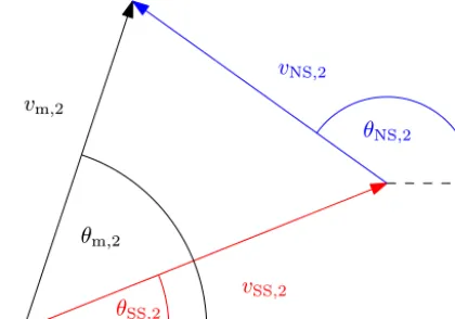
For the near-surface current, measurements close to the surface (e.g. vm,2) can be used. However, these
measure-ments include sub- and near-surface components, as shown in Fig. 3.
Therefore, the sub-surface component at 2 m has to be calculated using Eq. (7), and the sub-surface direction is assumed to be constant over depth (θSS,20=θSS,2=θSS,0).
calcu-0 0.2 0.4 0.6 0.8 1 0
10
20
Normalised current speed
Dep
th
belo
w
w
ater
sur
face Sub-surfaceNear-surface
Figure 2. Velocity profiles of the sub- and near-surface currents according to Eqs. (7) and (8) respectively, with a water depth of 25 m and normalised speeds (vSS,0=vNS,0=1).
late the near-surface current at 2 m:
vNS,2= q
v2SS,2+vm,22 −2vSS,2vm,2cos θm,2−θSS,2
, (10)
θNS,2=θm,2+arcsin vSS,2sin θm,2
−θSS,2
vNS,2 !
. (11)
Lastly, the reference near-surface currentvNS,0is given by
vNS,0=vNS,2
20 m
20 m−2 m
. (12)
A depth-independent near-surface direction is assumed, and thereforeθNS,0=θNS,2.
After having post-processed the measurement raw data, maximum likelihood estimations are applied to the processed data of the regarded 13 environmental conditions in order to fit several statistical distributions. In addition to unimodal distributions, and if several distinct peaks are distinguishable, multimodal distributions are fitted as well, as it is assumed that the peaks are due to physical phenomena. However, as multimodal approaches have more degrees of freedom, they always fit the data better, even in the case of a physically uni-modal shape. Therefore, they have to be chosen with care in order not to fit physically unimodal distributions with multi-modal approaches.
Considering the example of wind speed and wave height, it is self-evident that some environmental parameters are con-ditioned by others, and dependencies have to be defined. For example, the case of a calm sea during a storm is very un-likely. Analysing scatter plots of the environmental inputs and taking a literature review into account, the dependencies in Table 2 are defined, although it is possible to define them differently (see Stewart, 2016), as mainly the correlation is significant, and the determination of cause and effect is sec-ondary.
One of the most common ways to include dependencies in statistical distributions is to split up the data of the de-pendent parameters into several bins of the indede-pendent pa-rameters (e.g. Stewart, 2016; Johannessen et al., 2002; Li et
v m,2
v SS,2
v NS,2
θ SS,2
θ NS,2
θ m,2
Figure 3.Vectorial analysis of ocean current components at a depth of 2 m (measured values (m), near- and sub-surface components (NS and SS)).
al., 2015). To illustrate this approach, for example, the wave peak period is fitted in several bins of 0.5 m wave height (e.g.P(Tp)=P(Tp|1.5 m≤Hs<2 m)). The bin widths for the dependent parameters are summarised in Table 2 as well. For highly correlated parameters, an alternative to the bin-ning procedure is to model only the deviation between the parameters. Here, the direction of the near-surface current that is highly dependent on the wind direction is an exam-ple. Therefore, by modelling the deviation1NSaccording to
Table 2, the following applies:
θNS=1NS+θwind (13)
Visual inspections and objective criteria using Kolmogorov–Smirnov tests (KS tests) and chi-squared tests (χ2tests) are used to select the best fitting distribution for each environmental condition. Although the KS test is less powerful than other statistical tests, it is still used due to its suitability for small samples (occurring, for example, for dependent variables and high wind speeds), whereχ2
tests are not applicable. For one parameter, it is attempted to chose only one distribution for all bins and sites in order to keep the database easy to use. However, as noted in Table 2, in some cases several distributions are selected to increase the accuracy of the fits.
Directional parameters like θwind are treated differently, as classical, parametric distributions can hardly fit several peaks in continuous distributions (0◦=360◦). Therefore, a non-parametric kernel density estimation (KDE) is used to fit directional parameters.
2.3 Resulting distributions
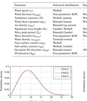
Table 2.Dependencies, statistical distributions, and bin widths for environmental conditions derived from FINO1–3 data.
Parameter Statistical distributions Dependencies Bin sizes
Wind speed (vs) Weibull – –
Wind direction (θwind) Non-parametric KDE Wind speed 2 m s−1 Turbulence intensity (TI) Weibull, gamma Wind speed 2 m s−1 Wind shear exponent (αPL) Bimodal normal Wind speed 2 m s−1
Air density (ρair) Bimodal log-normal – –
Significant wave height (Hs) Gumbel, Weibull Wind speed 2 m s−1
Wave peak period (Tp) Bimodal Gumbel Wave height 0.5 m
Wave direction (θwave) Non-parametric KDE Wave height and wind direction 1.0 m and 30◦
Water density (ρwater) Trimodal normal – –
Near-surface current (vNS) Weibull – –
Sub-surface current (vSS) Weibull, Gumbel – –
Deviation NS direction (1NS) Bimodal normal (Wind direction and NS direction) –
SS direction (θSS) Non-parametric KDE – –
0 5 10 15 20 25 30
0 0.02 0.04 0.06 0.08 0.1
Wind speed in m s−1
Pr
obability
density
FINO1 FINO2 FINO3
Figure 4. Weibull distributions for the wind speeds for all three sites.
due to the comprehensiveness of the data, detailed and addi-tional information is provided in an easily applicable form, in the Supplement. At this point, only two examples are shown in Figs. 4 and 5.
2.4 Special findings
In this section, some noteworthy findings of this database, mainly resulting from the consideration of scattering, are pointed out. Three examples are presented: the importance of wave peak periods, the high scattering of wind shear ex-ponents, and the behaviour of the turbulence intensity.
Wave loads are of particular importance if the wave fre-quency is close to the first natural frefre-quency of the struc-ture. Standard offshore wind turbines have first bending fre-quencies of about 0.25 to 0.3 Hz (Jonkman and Musial, 2010; Popko et al., 2012) corresponding to eigenperiods of less than 4 s. If state-of-the-art databases are used (see Ta-ble 1), there will be no resonance. However, real data sug-gest that resonance effects are problematic even for higher wind speeds, as wave peak periods of less than 4 s occur (see Fig. 6).
0 2 4 6 8
0 0.5 1
Wave height in m
Pr
obability
density
0 m s−1 ≤ 2 m s−1
6 m s−1 ≤ 8 m s−1
10 m s−1 ≤ 12 m s−1
20 m s−1 ≤ 22 m s−1 26 m s−1 ≤ 28 m s−1
Figure 5.Distribution of the significant wave height for different wind speeds and the FINO1 site. Forvs≤10 m s−1, Gumbel distri-butions are applied. For higher wind speeds, Weibull distridistri-butions fit the data more accurately.
Concerning the wind shear exponent, in the standards and most current databases (e.g. GL, 2012; Fischer et al., 2010), constant values for all wind speeds are proposed. However, this assumption is a massive simplification. Ernst and Seume (2012) showed that the wind shear exponent significantly de-pends on the wind speed. Here, it is shown (see Fig. 7) that it does not only vary between wind speeds but also scatters remarkably within each bin as well, and might even be nega-tive.
For the turbulence intensity, this database reveals that state-of-the-art approaches are mainly conservative, as too high turbulence intensities are assumed. This is shown in Fig. 8, where the turbulence intensity for all three sites is compared to a standard database (Fischer et al., 2010) and to current standards (IEC, 2009). All three sites exhibit sim-ilar mean turbulence intensities and 90th percentile values (Q0.9). For the comparison with literature values, the 90th
per-5 10 15 20 0
0.02 0.04 0.06 0.08
Wave peak period ins
Pr
obability
of
occur
rence
s
Figure 6. Probability distribution of the wave peak period for vs=11–13 m s−1for the FINO3 site.
−0 .10 0 0.1 0.2 0.3 0.4
5 10
Wind shear exponent
Pr
obability
density
2 m s−1 ≤ 4 m s−1
10 m s−1 ≤ 12 m s−1
20 m s−1 ≤ 22 m s−1
Figure 7.Distribution of the wind shear exponent for different wind speeds for the FINO2 site.
centile, the UPWINDdatabase is very conservative. The least conservative case (category C) in IEC (2009) fits the Q0.9
values relatively well, but it predicts slightly higher turbu-lence intensities for wind speeds above about 10 m s−1. Con-sidering the fact that using the 90th percentile is a conser-vative assumption and that the measurements include some wake effects due to wind farms near to all measurement masts, it can be concluded that state-of-the-art assumptions for turbulence intensities are probably unnecessarily conser-vative. The wake effects are depicted in Fig. 9, where turbu-lence intensity measurements of FINO1 from 2011 to 2016 are shown. In this period, the wind farm Alpha Ventus was operating on the east side of FINO1. Therefore, west wind leads to free stream conditions and east wind to wake con-ditions. Obviously, free stream conditions lead to even lower turbulence intensities, whereas wake conditions increase the turbulence, especially for smaller wind speeds, as also de-tected by Hansen et al. (2012).
3 Simulation assistance
In the previous section, a comprehensive database for scatter-ing environmental offshore conditions was developed. How-ever, even with realistic input parameters the accuracy of nu-merical simulations is significantly influenced by constraints like their lengths and the time eliminated to exclude
ini-5 10 15 20 25
0 0.1 0.2 0.3
Wind speed in m s−1
T
urbulence
intensity
FINO1 0.9,FINO1 FINO2 0.9,FINO2 FINO3 0.9,FINO3 UPWIND
Figure 8.Turbulence intensity (mean value and 90th percentile (Q0.9)) for different wind speeds compared to the literature.
tial transients. Therefore, in this section, efficient simulation lengths and times of initial transients for varying wind speeds and different types of loading and substructures are deter-mined. This is achieved by analysing the convergence of rel-evant quantities (i.e. FLS and ULS loads). Before conducting these studies, the overall probabilistic simulation approach is explained, as it differs from the approach in the standards. Subsequently, the utilised simulation model and the chosen environmental conditions are briefly presented.
3.1 Probabilistic simulation approach
For the design of offshore wind turbines, several design load cases (DLC1.1 to 8.3) have to be simulated according to the standards (IEC, 2009). These load cases cover ulti-mate and fatigue loads during power production, idling and fault conditions, and several special cases like start-up or shut-down. Stochastic inputs for turbulent wind and irregu-lar wind are included. Nevertheless, the DLCs remain quasi-deterministic, as environmental conditions like turbulence in-tensities and wind shear do not scatter. In order to guaran-tee safe designs despite the deterministic approach, several ULS load cases, covering extreme environmental conditions (e.g. DLC1.3 for turbulence or DLC1.5 for wind shear), are needed.
5 10 15 20 25 0
0.1 0.2 0.3
Wind speed in m s−1
T
urbulence
intensity
west 0.9,west
east 0.9,east
UPWIND
Figure 9.Shadow effects on the turbulence intensity for FINO1 and free stream (western) and wake (eastern) conditions.
and others are covered and do not have to be considered sep-arately. Load cases are not simulated explicitly, but are cov-ered implicitly by conducting probabilistic simulations.
That is why the two approaches do not differ significantly for FLS. The “real-life” approach covers DLC 1.2 and 6.4. For ULS, the “real-life” approach covers all power produc-tion cases (DLC 1.1–1.6) and DLC 6.1 by applying scattering environmental conditions. As the “real-life” approach cannot simulate 20 years of turbine lifetime (or even a return period of 50 years), a load extrapolation, as required for DLC 1.1, is needed in order to calculate an ULS design. However, this extrapolation is not needed here, as it does not influence the investigated simulation constraints.
As common in academia, only power production and idling is simulated. Fault cases, start-up, etc. are not taken into account due to several reasons. Firstly, at least for the jacket, fault cases are less relevant (Vemula et al., 2010). Secondly, these load cases are very controller and design de-pendent and need special treatment (e.g. there is no need of removing initial transients for start-up load cases). Thirdly, this work is not intended to calculate exact fatigue damages or ultimate loads for the whole turbine lifetime, as no tur-bine design or optimisation is done. The exclusion of some load cases does not affect the recommendations on simu-lation constraints that are given for power production and idling conditions. As there is no need of exact FLS and ULS lifetime loads in this study, an assessment of the probabilistic approach concerning accordance with the standards is neither conducted nor needed, but this would be valuable for further applications of probabilistic approaches.
3.2 Simulation setup
As environmental conditions vary for various turbine sites, a database being used for the studies of convergence has to be chosen. The basis developed in this work is appropriate, and the FINO3 site is chosen. Some conditions, like air and wa-ter density, are kept fixed, as it was shown that their variation
is of minor importance (Hübler et al., 2017). An attempt is made to keep the convergence study as simple as possible, and to focus on the most relevant parameters. Hence, for the probabilistic approach, statistically scattering values accord-ing to the determined distributions of wind speed and direc-tion, wave height, direction and period, turbulence intensity, and wind shear exponent are used in all simulations. In addi-tion, the following assumptions are made for all simulations:
– The turbulent wind field is computed according to the Kaimal model and using the software TurbSIM (Jonkman, 2009) with a different wind seed for each simulation.
– Irregular waves are calculated according to the JON-SWAP spectrum using varying wave seeds for all simu-lations.
– Soil conditions of the OC3 model (Jonkman and Musial, 2010) are applied.
– The current, second-order and breaking waves, wave spreading effects, marine growth, local vibration effects of braces, joint stiffnesses, and degradation effects are neglected.
The time domain simulations of the convergence study are conducted using the aero-servo-hydro-elastic simulation framework FASTv8 (Jonkman, 2013). A soil model (Häfele et al., 2016) applying linearised soil-structure interaction ma-trices enhances this code. The NREL 5 MW reference wind turbine (Jonkman et al., 2009) with two different substruc-tures is investigated: Firstly, the OC3 monopile (Jonkman and Musial, 2010) and secondly, the OC4 jacket (Vorpahl et al., 2013). The outcomes of the FAST simulations are, in-ter alia, time series of forces, moments, and stresses for each element of the substructure.
Since the convergence of fatigue and ultimate loads is in-vestigated in the next step, the calculation concept of these two loads is briefly explained.
joint is necessary, as damages in each connection and joint are different for each simulation, and the highest values do not always occur in the same joint (for example due to the probabilistic variation of the wind direction). Finally, the de-cisive damage for the jacket is the highest accumulated value of all connections of all joints.
For the monopile, the fatigue procedure is similar, but is done according to European Committee for Standardization (2010b), where a detail of 71 MPa for transverse butt welds and an additional reduction due to the size effect (t >25 mm) is recommended. Differing from the recommendations in European Committee for Standardization (2010b), the same slopes of the S–N curves as for the jacket are used.
For the ULS analysis, maximum stresses are decisive and extracted from the time series. For the monopile, European Committee for Standardization (2010a) is used to analyse the plastic limit state, cyclic plasticity limit state, and buckling limit state (LS1–3). For the jacket, NORSOK N-004 is ap-plied for tubular members and joints, which takes combined axial, shear, bending, and hydrostatic loadings into account. In both cases, the yield stress is 355 MPa.
Additionally, ultimate limit state proofs for the foundation piles are performed including axial and lateral soil proofs ac-cording to GEO2 (DIN 1054, 2010) and a plastic limit state proof (LS1) for the steel pile below mudline. Especially for the monopile, the last proof might be decisive as the bend-ing moment frequently reaches its maximum below mudline. For all ULS proofs, utilisation factors, being the percentage of the maximum loads, are the outcomes.
3.3 Simulation length
The simulation length significantly influences the overall computing time of the load assessment. However, there is no conclusive consensus concerning the length needed. Cur-rent standards recommend, for example, 10 min or 1 h calcu-lations. The offshore oil and gas industry prefers simulation lengths of 6 h to cover all low-frequency hydrodynamic ef-fects.
The use of 10 min simulations can potentially reduce the computing time by a factor of about 36 compared to 6 h sim-ulations. Hence, a study of convergence for bottom-fixed off-shore wind turbines is conducted here. For floating wind tur-bines, it is referred to Stewart (2016), who showed that for floating structures all physical effects can be covered with 10 min simulations.
The presented outcomes of this study focus on the monopile substructure, but a jacket is analysed as well and results (not shown) are generally comparable. For several wind speed bins, 500 simulations with a total length of 10 h are conducted. As the initial transient behaviour is analysed subsequently, a clearly sufficient time, being discarded to ex-clude the initial transients, of 4 h is chosen. With elimination of these 4 h of initial transients, the total length of 10 h re-duces to a maximum available length (simulation length) of
6 h for the convergence study. In a first step, the convergence of FLS loads is analysed. Afterwards, the ULS case is inves-tigated.
The procedure to calculate the mean fatigue damage for each wind speed bin is the following: from the basis of the 500 ten-hour simulations having different random seeds and varying environmental conditions, 500 cases are selected (with replacement). For each simulation, the fatigue damage is calculated and weighted with the simulation length. The mean value of all cases is calculated. This procedure is re-peated 10 000 times (bootstrapping) to assess the associated uncertainty.
Figure 10 displays the normalised mean fatigue damages for different wind speeds and simulation lengths between 10 min and 6 h. The values are normalised with the 6 h val-ues, and error bars show the±σ confidence intervals (68 %) that are estimated using a bootstrap procedure with 10 000 re-samplings.
10 min 30 min 1 h 2 h 6 h 0.8
1 1.2 1.4 1.6
Simulation length
N
or
malised
mean
fatigue
damag
e
0–3 m s−1 9–11 m s−1 15–17 m s−1
Figure 10.Normalised mean fatigue damage (500 simulations) for increasing simulation lengths and different wind speeds.
10 min 30 min 1 h 2 h 6 h
0.95 1 1.05
Simulation length
N
or
malised
mean
fatigue
damag
e
Not merged Merged
Figure 11.Normalised mean fatigue damage (500 simulations) for increasing simulation lengths andvs=9–11 m s−1. Environmental conditions are kept constant to demonstrate the effect of merging time series more clearly.
unreasonably increased fatigue damages. Merging each time series with itself guarantees fitting load levels. A downside of this is that the computing time of the post-processing is slightly increased. The effect of merging several shorter sim-ulations with themselves to generic and repetitive 6 h time se-ries (e.g. each 10 min time sese-ries is duplicated 36 times and is appended to itself to create a 6 h time series) is demon-strated in Fig. 11. It can be seen that the simulation error of about 5 % too low FLS loads for non-merged 10 min simula-tions can be compensated for by merging time series in the post-processing.
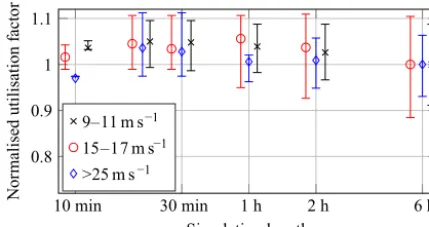
For the ULS loads, the calculation procedure is similar. From the basis of the 500 ten-hour simulations, 500 cases are selected (with replacement). The maximum value of all simulations is taken as decisive utilisation factor. This pro-cedure is repeated 10 000 times (bootstrapping) to assess the associated uncertainty.
The convergence is shown in Fig. 12. Obviously, ULS loads are higher for longer simulations. Again, this increase is not due to any physical phenomenon, but a result of differ-ent overall computing times. Clearly, 500 ten-minute simula-tions should not be compared to 500 six-hour simulasimula-tions but
10 min 30 min 1 h 2 h 6 h
0.8 0.9 1 1.1
Simulation length
N
or
malised
utilisation
fact
or 9–11 m s−1 15–17 m s−1 >25 m s−1
Figure 12.Normalised mean ULS utilisation factor (500 simula-tions) for increasing simulation lengths and different wind speeds.
instead to about 14 six-hour simulations (Haid et al., 2013). Therefore, in a second step, the ULS calculation procedure is slightly adapted. Now, 500 cases are only selected for 10 min simulations. For all other simulations length, the number of cases is reduced to keep the over simulation length constant at 5000 min (i.e. 250 cases for 20 min simulation, for exam-ple). This comparison is displayed in Fig. 13 and makes clear that ULS loads do not depend on the simulation length but in-stead on the overall computing time. A second fact being vis-ible in Fig. 13 are the higher uncertainties for longer simula-tion lengths. Since 10 min simulasimula-tions lead to a higher num-ber of cases than 6 h simulations for the same total length (i.e. 500 and 14), shorter simulations better cover rare cases, and therefore scattering environmental conditions leading to less uncertainty.
After all, the investigations of this section suggest that sim-ulations of 10 min length are sufficient independent of the type of load or investigated substructure, or wind speed. At this point, it has to be noted that only two types of substruc-tures are analysed and environmental conditions typical for the North Sea. For significantly different substructures or lo-cations, the validity might be limited. Notwithstanding the above, for ULS loads, the same overall time has to be com-pared in order to achieve reliable results. By keeping the sim-ulation length short, more simsim-ulations can be conducted in the same overall computing time leading to a better conver-gence of ULS loads. For FLS loads, simulation errors due to the simulation length can be reduced by merging the time series.
3.4 Initial transients
10 min 30 min 1 h 2 h 6 h 0.8
0.9 1 1.1
Simulation length
N
or
malised
utilisation
fact
or
9–11 m s−1 15–17 m s−1 >25 m s−1
Figure 13.Normalised mean ULS utilisation factor for increasing simulation lengths (constant overall length of 500×10 min, leading to 500 to 14 simulations) and different wind speeds.
rotor speeds and blade pitches depending on the wind speed are set here. These initial conditions are quasi-static states determined using prior simulations.
As the initial transient behaviour is affected by the type of substructure and the load condition, the time that has to be re-moved is analysed in each wind speed bin for FLS and ULS loads and for both types of substructures separately. Com-monly, time series are investigated to estimate times of ini-tial transients (Zwick and Muskulus, 2015). Although this is a straightforward approach, here it is considered to not be expedient. For a fatigue assessment, the convergence of the fatigue damage has to be analysed, and for the ULS analysis, maximum loads or utilisation factors have be considered.
For each wind speed bin, 10 000 simulations for the monopile and 500 for the jacket were conducted according to the simulation setup in Sect. 3.2. This means that each simu-lation has its own random seed for irregular waves and turbu-lent wind, and in addition, different wind speeds and direc-tions, wave heights, directions and periods, turbulence inten-sities and wind shear exponents according to the FINO3 data are applied. The high and unequal number of simulations is needed to exclude effects of the number of simulations, mentioned in the previous section and addressed in Sect. 4, as well as possible. For the monopile, each simulation at operating conditions is 900 s long (600 s simulation length plus 300 s of initial transients) and 1800 s at idling condi-tions. When the turbine is idling, the aerodynamic damping is lower, leading to more pronounced initial transients. For the jacket, all simulations are 720 s long. Using this simu-lated database, it is possible to analyse the effect of different initial simulation times removed on the fatigue damage and utilisation factors in order to determine optima. The analysed simulation length is kept constant at 600 s, while the removed length varies between 0 and 300 s (1200 s for idling; 120 s for the jacket).
Figure 14 displays the convergence of the fatigue damage of the monopile substructure at operating conditions. Here, 300 s or 120 s values are used as a reference, the so-called “converged value”. The 10 h simulations in Sect. 3.3 were
50 100 150 200 250 300 0
10 20 30
Initial simulation time removed in s
P
er
cent
ag
e
differ
ence
in
fatigue
damag
e
9–11 m s−1
15–17 m s−1
17–19 m s−1
23–25 m s−1
Figure 14.Initial transient behaviour of the operating wind turbine with a monopile substructure for different wind speeds. Percentage difference in the fatigue damage compared to the “converged” value (300 s).
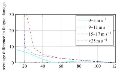
used determine these values, where the error due to initial transients can be neglected and is much smaller than the er-ror due to the number of simulations. For idling conditions (not shown), the initial transient behaviour takes longer, as the aerodynamic damping is lower. For the same reason, the transients are shorter for higher wind speeds. For the jacket substructure displayed in Fig. 15, the transients decay much faster in all wind speed bins. As jackets are less influenced by wave loads, being not always aligned with the wind, the aerodynamically marginally damped side-to-side modes are less excited, leading to a shorter transient behaviour. This in-terpretation is supported by the fact that for the jacket, idling conditions, where the hydrodynamic behaviour dominates, have shorter initial transients.
The convergence of ULS utilisation factors for both sub-structures is shown in Figs. 16 and 17. It becomes apparent that initial transients are short independent of the type of sub-structure and wind speed. The cycles with high amplitudes occurring at the beginning of each simulation are damped out within a few seconds, and hence are not influencing the ULS behaviour. More problematic are less damped cycles with smaller amplitudes leading to the previously presented, higher times of initial transients for FLS loads.
Table 3.Recommended times that should be discarded to exclude initial transients for simulations with OC4 jacket and OC3 monopile substructures for different wind speeds to achieve errors below 5 %.
vsin m s−1 Case <3 3–5 5–7 7–9 9–11 11–13 13–15 15–17 17–19 19–21 21–23 23–25 >25
Monopile
FLS 720 s 240 s 240 s 240 s 240 s 240 s 240 s 150 s 120 s 60 s 60 s 60 s 360 s Jacket 40 s 30 s 50 s 40 s 50 s 50 s 50 s 50 s 50 s 60 s 50 s 50 s 10 s
Monopile
ULS <10 s <10 s <10 s <10 s 10 s 10 s 10 s 10 s 10 s 10 s 10 s 10 s <10 s Jacket <10 s 20 s 20 s 20 s 20 s 20 s 20 s 20 s 20 s 20 s 20 s 20 s <10 s
20 40 60 80 100 120
0 10 20 30
Initial simulation time removed in s 0–3 m s−1 9–11 m s−1 15–17 m s−1 >25 m s−1
Figure 15. Initial transient behaviour of the wind turbine with a jacket substructure for different wind speeds. Percentage difference in the fatigue damage compared to the “converged” value (120 s).
20 40 60 80 100 120
0 2 4 6 8 10
Initial simulation time removed in s
3–5 m s−1
9–11 m s−1
17–19 m s−1
23–25 m s−1
Figure 16. Initial transient behaviour of the wind turbine with a monopile substructure for different wind speeds. Percentage differ-ence in the utilisation factor (ULS) compared to the “converged” value (120 s).
Zwick and Muskulus, 2015 or Morató et al., 2017), the given values represent a well-founded guidance for simulation se-tups. Furthermore, these results should sensitise the research community to the problem of initial transients especially in the case of fatigue. For fatigue, the time of initial transients might be higher than frequently presumed in the literature. This is due to weakly damped cycles with small amplitudes that cannot directly be identified when looking at time series.
20 40 60 80 100 120
0 2 4 6 8 10
Initial simulation time removed in s 3–5 m s−1 9–11 m s−1 17–19 m s−1 23–25 m s−1
Figure 17.Initial transient behaviour of the wind turbine with a jacket substructure for different wind speeds. Percentage difference in the utilisation factor (ULS) compared to the “converged” value (120 s).
4 Benefits and limitations
The benefit of the current work is twofold. Firstly, a com-prehensive database for scattering environmental conditions was set up, which is freely available and easy to use. Sec-ondly, two simulation constraints (simulation length and time of initial transients) were analysed, and well-founded recom-mendations are given.
For example, wind speeds are measured at heights compara-ble to hub heights of current turbines, and there is no need for extrapolations, as is the case for buoy measurements. Still, more data would be valuable in order to achieve more reli-able distributions in high-wind-speed bins that rarely occur. After all, the developed database is capable of improving offshore wind turbine modelling by providing more realis-tic inputs for simulations in academia, where real site data are scarce. One example of improved offshore wind turbine modelling is given in Sect. 3.3 and 3.4. The inclusion of prob-abilistic inputs leads to a significant and realistic increase in fatigue damage scattering requiring high numbers of simula-tions. Hence, deterministic inputs underestimating this scat-tering can lead to biased fatigue values. Detailed analyses of the effect of scattering environmental conditions on fatigue damage, and therefore of the needed number of simulations, are part of upcoming work of the authors.
Concerning the second benefit, the simulation constraints, it has to be kept in mind that not only realistic modelling but also small simulation errors are important in order to model accurately. In this context, the chosen simulation length and time of initial simulation transients matter. So far, these values are frequently chosen without profound knowledge. Some approaches to gain a deeper insight into these con-straints (Stewart, 2016; Zwick and Muskulus, 2015) concen-trate on simulation lengths or specific types of substructures and are not taking realistically scattering environmental ditions into account. In this work, the scattering of the con-ditions is addressed and different bottom-fixed substructures are analysed. This enables recommendations for simulation lengths and times of initial transients depending on the wind speed, the type of substructure, and the considered load case (ULS or FLS). However, the general validity of the current results has to be slightly restricted, as only one design of each type of substructure was investigated. Therefore, the initial transient behaviour might be slightly different for sig-nificantly different designs. Furthermore, for the time be-ing removed to exclude initial transients, the values might also differ between different simulation codes and are only tested for the FASTv8 code. Different numerical solver or time constants of the aero-elastic models might also influ-ence the time of initial transients. Nevertheless, even in these cases, firstly, the given recommendations can be regarded as a well-founded starting point for further investigations. Sec-ondly, and even more important, they clarify the challenge of a well-founded choice.
5 Conclusions
This work aims to help future simulation work to be more re-alistic and accurate. In order to achieve this objective, a freely available and comprehensive database for scattering environ-mental conditions was set up. This database consists of con-ditional statistical distribution for many parameters and can
be applied without further post-processing. All needed infor-mation (statistical distribution and their parameters) is given in the Supplement. In academia, this database enables sim-ulations with probabilistic environmental conditions making them more realistic. For industry purposes, this work might lead to a reconsideration of the current practice. This study shows that the use of deterministic values that are either only dependent on the wind speed (e.g. turbulence intensity) or even totally constant (e.g. wind shear) does not represent alistic offshore conditions. However, for a well-founded re-consideration of the current practice, a detailed assessment of probabilistic approaches compared to deterministic load-case-based ones is needed.
Additionally, scientifically sound recommendations are given for the choice of simulation lengths and times to be removed to exclude initial transients. Simulation lengths of 10 min are generally sufficient, and can even help to reduce uncertainties. However, in the case of FLS loads, times se-ries should be merged, and for ULS situations, the overall computing time has to be kept constant. Recommendations concerning the initial transients have to be handled with care due to limitations of the general validity. The values are sum-marised in Table 3 and can help to improve the accuracy of simulations, and to reduce computing times. It should be noted that a partly significantly longer initial transient be-haviour compared to values in the literature was detected. Literature values are mainly based on educated guesses so far.
An enlargement of the current database to include addi-tional offshore sites, other types or designs of substructures, or investigations for other simulation codes and numerical solver would be definitely valuable to increase the general validity. Furthermore, even for the utilised FAST code, ad-ditional investigations concerning the amount of eigenmodes representing the substructure would be beneficial, as a reduc-tion of retained eigenmodes might reduce the time of initial transients.
Data availability. The raw data are taken from the FINO plat-forms – operated on behalf of the Federal Ministry for the Environ-ment, Nature Conservation, Building and Nuclear Safety (BMUB) – and are freely available for research purposes (http://www. fino-offshore.de/en/). The derived database, consisting of statisti-cal distribution for 13 partly dependent environmental conditions and three offshore sites, is freely available. All needed information concerning the statistical distribution and their parameters is given in the Supplement.
Competing interests. The authors declare that they have no con-flict of interest.
Acknowledgements. We gratefully acknowledge the financial support of the Lower Saxony Ministry of Science and Culture (research project VENTUS EFFICIENS, FKZ ZN3024) and the European Commission (research project IRPWIND, funded from the European Union’s Seventh Framework Programme for research, technological development, and demonstration under grant agreement number 609795) that enabled this work. This work was supported by the compute cluster which is funded by Leibniz Universität Hannover, the Lower Saxony Ministry of Science and Culture (MWK), and the German Research Foundation (DFG).
The publication of this article was funded by the open-access fund of Leibniz Universität Hannover.
Edited by: Michael Muskulus Reviewed by: two anonymous referees
References
Cheng, P. W.: A reliability based design methodology for extreme responses of offshore wind turbines, DUWIND Delft University Wind Energy Research Institute, the Netherlands, 2002. Det Norske Veritas (DNV): Fatigue design of offshore steel
structures, Recommended practice DNV-RP-C203, available at: https://rules.dnvgl.com/docs/pdf/DNV/codes/docs/2010-04/ RP-C203.pdf (last access: October 2017), 2010.
Det Norske Veritas (DNV): Design of floating wind turbine structures, Offshore Standard DNV-OS-J103, available at: http://rules.dnvgl.com/docs/pdf/DNV/codes/docs/2013-06/ OS-J103.pdf (last access: October 2017), 2013.
DIN – Normenausschuss Bauwesen: Subsoil – Verification of the safety of earthworks and foundations – Supple-mentary rules to DIN EN 1997-1, DIN 1054, available at: https://www-1perinorm-1com-100000boj285b.shan02.han.tib. eu/document.aspx (last access: October 2017), 2010.
Ernst, B. and Seume, J. R.: Investigation of site-specific wind field parameters and their effect on loads of offshore wind turbines, Energies, 5, 3835–3855, 2012.
European Committee for Standardization: Eurocode 3: Design of steel structures – Part 1–6: Strength and stability of shell struc-tures, EN 1993-1-6, Brussels, Belgium, 2010a.
European Committee for Standardization: Eurocode 3: Design of steel structures – Part 1–9: Fatigue, EN 1993-1-9, Brussels, Bel-gium, 2010b.
Fischer, T., de Vries, W., and Schmidt, B.: Upwind Design Basis, Endowed Chair of Wind Energy (SWE) at the Institute of Aircraft Design Universität Stuttgart, Germany, 2010.
Germanischer Lloyd (GL): Guideline for the Certification of Off-shore Wind Turbines, OffOff-shore Standard, Hamburg, Germany, 2012.
Häfele, J., Hübler, C., Gebhardt, C. G., and Rolfes, R.: An improved two-step soil-structure interaction modeling method for dynam-ical analyses of offshore wind turbines, Appl. Ocean Res., 55, 141–150, 2016.
Häfele, J., Hübler, C., Gebhardt, C. G., and Rolfes, R.: Effcient Fa-tigue Limit State Design Load Sets for Jacket Substructures Con-sidering Probability Distributions of Environmental States, The 27th International Ocean and Polar Engineering Conference, 25– 30 June 2017, San Francisco, USA, 167–173, 2017.
Haid, L., Stewart, G., Jonkman, J., Robertson, A., Lackner, M., and Matha, D.: Simulation-length requirements in the loads analy-sis of offshore floating wind turbines, 32nd International Con-ference on Ocean, Offshore and Arctic Engineering, 9–14 June 2013, Nantes, France, 1–10, ASME, 2013.
Hansen, K. S., Barthelmie, R. J., Jensen, L. E., and Sommer, A.: The impact of turbulence intensity and atmospheric stability on power deficits due to wind turbine wakes at Horns Rev wind farm, Wind Energy, 15, 183–196, 2012.
Hansen, M., Schmidt, B., Ernst, B., Seume, J., Wilms, M., Hilde-brandt, A., Schlurmann, T., Achmus, M., Schmoor, K., Schau-mann, P., Kelma, S., Goretzka, J., Rolfes, R., Lohaus, L., Werner, M., Poll, G., Böttcher, R., Wehner, M., Fuchs, F., and Brenner, S.: Probabilistic Safety Assessment of Offshore Wind Turbines, Leibniz Universität Hannover, Hannover, Germany, 2015. Hübler, C., Gebhardt, C. G., and Rolfes, R.: Hierarchical Four-Step
Global Sensitivity Analysis of Offshore Wind Turbines Based on Aeroelastic Time-Domain Simulations, Renew. Energ., 111, 878–891, 2017.
International Electrotechnical Commission (IEC): Wind turbines – part 1: Design requirements, International standard IEC 61400-1, Geneva, Switzerland, 2005.
International Electrotechnical Commission (IEC): Wind turbines – part 3: Design requirements for offshore wind turbines, Interna-tional standard IEC 61400-3, Geneva, Switzerland, 2009. Johannessen, K., Meling, T. S., and Hayer, S.: Joint distribution for
wind and waves in the northern north sea, Int. J. Offshore Polar, 12, 1–8 2002.
Jonkman, B. J.: TurbSim user’s guide: Version 1.50, National Re-newable Energy Laboratory, Golden, Colorado, USA, 2009. Jonkman, J.: The New Modularization Framework for the FAST
Wind Turbine CAE Tool, 51st AIAA Aerospace Sciences Meet-ing, including the New Horizons Forum and Aerospace Exposi-tion, 7–10 January 2013, Dallas, Texas, USA, 1–26, 2013. Jonkman, J., Butterfield, S., Musial, W., and Scott, G.: Definition
of a 5 MW Reference Wind Turbine for Offshore System Devel-opment, National Renewable Energy Laboratory, Golden, Col-orado, USA, 2009.
Jonkman, J. M. and Musial, W.: Offshore Code Comparison Collab-oration (OC3) for IEA Task 23 Offshore Wind Technology and Deployment, National Renewable Energy Laboratory, Golden, Colorado, USA, 2010.
Kost, C., Mayer, J. N., Thomson, J., Hartmann, N., Senkpiel, C., Philipps, S., Nold, S., Lude, S., and Schlegl, T.: Stromgeste-hungskosten erneuerbare Energien, Fraunhofer-Institut für solare Energiesysteme ISE, Freiburg, Germany, 2013.
Li, L., Gao, Z., and Moan, T.: Joint distribution of environmental condition at five european offshore sites for design of combined wind and wave energy devices, J. Offshore Mech. Arct., 137, 031901, https://doi.org/10.1115/1.4029842, 2015.
Morató, A., Sriramula, S., Krishnan, N., and Nichols, J.: Ultimate loads and response analysis of a monopile supported offshore wind turbine using fully coupled simulation, Renew. Energ., 101, 126–143, 2017.
Popko, W., Vorpahl, F., Zuga, A., Kohlmeier, M., Jonkman, J., Robertson, A., Larsen, T. J., Yde, A., Saetertro, K., Okstad, K. M., Nichols, J., Nygaard, T. A., Gao, Z., Manolas, D., Kim, K., Yu, Q., Shi, W., Park, H., and Vásquez-Rojas, A.: Offshore Code Comparison Collaboration Continuation (OC4), Phase 1 – Results of Coupled Simulations of an Offshore Wind Turbine With Jacket Support Structure, The Twenty-second International Offshore and Polar Engineering Conference, International Soci-ety of Offshore and Polar Engineers, 17–22 June 2012, Rhodes, Greece, 337–346, 2012.
Prognos AG and Fichtner: Kostensenkungspotenziale der Offshore-Windenergie in Deutschland, Stiftung Offshore-Offshore-Windenergie, Berlin, Germany, 2013.
Stewart, G. M.: Design Load Analysis of Two Floating Off-shore Wind Turbine Concepts, PhD thesis, University of Mas-sachusetts, MasMas-sachusetts, USA, 2016.
Stewart, G. M., Lackner, M., Haid, L., Matha, D., Jonkman, J., and Robertson, A.: Assessing fatigue and ultimate load uncer-tainty in floating offshore wind turbines due to varying simula-tion length, Safety, Reliability, Risk and Life-Cycle Performance of Structures and Infrastructures, CRC Press, London, UK, 239– 246, 2013.
Stewart, G. M., Robertson, A., Jonkman, J., and Lackner, M. A.: The creation of a comprehensive metocean data set for offshore wind turbine simulations, Wind Energy, 19, 1151–1159, 2015. Vemula, N. K., de Vries, W., Fischer, T., Cordle, A., and Schmidt,
B.: Design Solution for the UpWind Reference Offshore Support Structure – Deliverable D4.2.5 (WP4: Offshore Foundations and Support Structures), Rambøll Wind Energy, Esbjerg, Denmark, 2010.
Vorpahl, F., Popko, W., and Kaufer, D.: Description of a basic model of the “UpWind reference jacket” for code comparison in the OC4 project under IEA Wind Annex 30, Fraunhofer IWES, Bre-merhaven, Germany, 2013.