R
R
O
O
B
B
U
U
S
S
T
T
F
F
A
A
C
C
T
T
O
O
R
R
B
B
A
A
S
S
E
E
D
D
A
A
N
N
O
O
M
M
A
A
L
L
Y
Y
D
D
E
E
T
T
E
E
C
C
T
T
I
I
O
O
N
N
I
I
N
N
H
H
I
I
E
E
R
R
A
A
R
R
C
C
H
H
I
I
C
C
A
A
L
L
W
W
I
I
R
R
E
E
L
L
E
E
S
S
S
S
S
S
E
E
N
N
S
S
O
O
R
R
N
N
E
E
T
T
W
W
O
O
R
R
K
K
S
S
B
B
a
a
r
r
a
a
k
k
k
k
a
a
t
t
h
h
N
N
i
i
s
s
h
h
a
a
U
U
.
.
11,
,
U
U
m
m
a
a
M
M
a
a
h
h
e
e
s
s
w
w
a
a
r
r
i
i
N
N
.
.
22,
,
V
V
e
e
n
n
k
k
a
a
t
t
e
e
s
s
h
h
R
R
.
.
33,
,
Y
Y
a
a
s
s
i
i
r
r
A
A
b
b
d
d
u
u
l
l
l
l
a
a
h
h
R
R
.
.
441, 2, 3
PSNA College of Engg& Technology, Department of Computer Science
4
Sri Subramaniya Colleges of Engg& Technology, Department of Computer Science
ABSTRACT: To improve data reliability, accuracy and to make effective and correct decisions using data collected from the wireless sensor network, it is necessary to detect the inconsistent data (outlier) caused by compromised or malfunctioning nodes. Data aggregation is augmented to eliminate the outlier data in the sensor network by multivar iate analysis technique such as factor analysis and mahalanobis distance. Factor analysis is a way to fit a model to multivar iate data to estimate the interdependence. In a factor analysis model, the measured variables depend on a smaller number of unobserved (latent) factors. The mahalanobis distance is used to determine the similarity of a set of values from an unknown samp1e to a set of values measured from a collection of known samples. Combined with factor analysis, Mahalanobis distance is extended to examine whether a given vector is an outlier from a model identified by factors based on factor analysis. In this paper to ensure accuracy during the aggregation process, factor analysis and mahalanobis distance methodologies are used and the data inconsistency is optimized. The performance graph shows that the Factor analysis and mahalanobis distance detects outlier better than the principal component analysis and subspace methods.
KEYWORDS: Aggregation, Distance Measure, Factors, Outlier, Sensor Network.
1.
INTRODUCTIONThe Wireless Sensor Networks (WSNs) are autonomous networks consisting of a large number of sensor nodes. WSNs consist of hundreds or even thousands of resource constrained nodes. Sensor is a small, lightweight device which measures the environment of physical parameters such as temperature, pressure, relative humidity etc. Sensor nodes are applied to perform measurements of some physical phenomena [Aky02]. Due to the hostile operation of sensor networks the sensor nodes are at risk to attacks, leading to the injection of false data into the network. This makes the data received at base station inconsistent with the observed phenomena or data. Thus the data integrity and accuracy becomes a major issue [CES04]. WSNs are powerful paradigm for many applications such as target tracking in battlefields, habitat monitoring in forest, environmental control and emergency response system. It is also employed in several real time monitoring systems like weather monitoring
[Sze04], environmental monitoring, vehicle tracking etc. Due to the critical nature of such applications, data integrity and accuracy problems become major issues in WSNs. To keep data reliability and accuracy high and be able to make effective and correct decisions using data collected by WSNs, the problem of erroneous data due to the existence of either compromised or faulty nodes in the network becomes of higher importance when data aggregation occurs. In WSNs neighbor nodes sends data to the aggregator nodes. Processing, caching and filtration are done by aggregator nodes to get meaningful information and thus by resending to sink nodes. Raw data are collected by aggregators from the remaining nodes in the cluster and summarizing is done by them to make the data usable. Unnecessary transmissions are eliminated from multiple sensors by aggregating the data and sending accurate information to the base station is called data aggregation in case of WSN's. Redundancies and faults are eliminated using aggregation to improve the level of accuracy [WDA09]. Thus performing aggregation can eliminate the redundancy and erroneous in data and there by improving the level of accuracy. Outliers are the metrics used to calculate the erroneous data, which deviates from the normal pattern of any sensor's data in WSN's.
2. RELATED WORK
Most of research efforts presented in the literature have discussed the problem of developing of efficient data aggregation mainly for energy savings and minimization in sensor networks [BS07, JSF06]. Prior work has rarely been concerned with the delay of aggregation and accuracy together. In [TH05] , a spatial-temporal correlation analysis called “abnormal relationships test” (ART) is proposed, to detect outliers in the collected data. This method is based on correlation coefficient tests between neighboring nodes. Each node stores the tests in a moving window, so any neighbour that starts reporting deviating values that exceed a predefined threshold is marked. Detection is achieved with collaboration between the nodes so as to isolate the problematic nodes.
The authors in [CP07, C+06, C+10b] have adopted principal component analysis (PCA) for dimension reduction and SPE to perform fault detection in the residual space. Since SPE is sensitive to modeling errors, it could increase the false alarm rate. However, that technique requires the complete knowledge of the density distribution function of the collected data. The authors in [C+10a] design a resilient aggregation using a robust estimation obtained from data distribution based on a statistical method.
The proposed approach affords an incorporated technique of taking into consideration and merging effectively correlated sensor data, in a distributed hierarchical network, in order to disclose outliers from the large dataset.
3. SYSTEM MODEL AND ARCHITECTURE
A sensor network is usually represented by a network graph. An algorithm that correlates metrics from neighbouring sensors is considered, to detect the nodes containing anomalies in the corresponding network graph. In order to decentralize the detection algorithm, the sensor network is divided into groups of sensors. Each group is controlled by a single coordinator. Coordinator is the responsible for processing the sensed data from the normal nodes in the group. Coordinators do the role of aggregator which aggregates and transmit data to the base station. This aggregation process reduces the energy consumption in order to avoid unwanted data transmission.
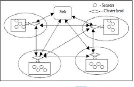
Figure 1 shows a cluster based sensor network organization. The cluster heads can communicate with the sink directly via long range transmissions or multi hopping through other cluster heads. In cluster based approach, sensor nodes is divided into towards the base station through a specific node called Cluster
Head (CH) taking care about the data aggregation from ambient nodes. All nodes in the specific cluster send its measured data to assigned CH performing the summarization and aggregation tasks and transmit an aggregated message to another CH or directly to the base station.
Figure 1. Cluster based sensor Network
4. MULTIVARIATE OUTLIER DETECTION
The objective of the multivariate outlier detection algorithm is to provide an efficient and effective methodology of combining data of heterogeneous monitors that spread throughout the network and analyzing interdependencies between variables in the data set. Outlier detection is possible only when multivariate analysis is performed, and the interactions among different variables are compared within the class of data [HCB00]. In this paper, we propose factor analysis as a multivar iate technique to identify the linear relationships among the observed variables and model the normal pattern of sensor data. The technique is augmented with mahalanobis distance measure to detect and isolate the inconsistent data.
4.1 Factor Analysis
Factor Analysis (FA) technique is used to identify the correlated relationship among the set of variables. The hidden model helps to analyze the multivariate data. It is used to expose the dimensions of a set of variables and larger number of variables to a smaller number of factors [JW98, AB06]. Factor analysis deals with a set of interpretations obtained from a given sample, analyzing the set of data with their correlations and evaluate the deviation compared with previous samples.
shared in common with more than one observed variable. Unique factors have effects that are unique to a specific variable. Being a branch of multivariate analysis, Factor Analysis offers a conceptual framework within which many disparate methods can be unified and a base from which new methods can be developed.
Let X be the observable random vector with m variables Xl, X2,,. ..,Xn that have mean and
covariance matrix . The factor model postulates that X is linearly dependent on a few unobservable random variables Fl, F2... Fp, called common factors,
and m additional sources of variation el, e2... em,
called errors, or specific factors. The factor analys is model is as follows:
or, in matrix notation
The coefficient , is called the loading of the ith variable on the jth factor, so the matrix L is the matrix of factor loadings. The ith specific factor is associated only with the ith .response . The p
deviations are expressed in
terms of m+p random variables F1, F2... Fp, el, e2...
em, which are unobservable. If assume the
unobservable random vectors F and e satisfy the following conditions:
The orthogonal factor model implies a covariance structure for X. From the model
So that,
From the covariance calculation,
so
Thus, we can get covariance structure for the orthogonal factor model:
The portion of the variance of the ith variable contributed by the m common factors is called the ith communality.
4.1.1 Methods of parameter estimation
The principal component factor analysis of the sample covariance matrix S is specified in terms of its eigenvalue-eigenvector pairs where,
Let be the number of common factors. Then the matrix of estimated factor loadings { } is given by
the estimated specific variance are provided by the diagonal elements of the matrix so
Communalities are estimated as
for a given factor do not change as the number of factors is increased. For example, if
and if p=2 , where and
are the first two eigen value-eigenvector pairs for S (or R). The principal component method satisfies
Factor scores are estimates of values for the unobserved random factor vector , j= l... n. That is, factor scores
= estimate of the values attained by Since the unobserved quantities and , outnumber the observed , some approaches to estimating factor values have been proposed including the weighted least squares method and the regression method.
where,
is the sample mean.
4.1.2 Shaping the quantity of factors
The number of factors can be determined based on the following approaches.
a) Kaiser decisive factor: The Kaiser decisive factor
is the default method to detect number of factors. It eliminates all components with eigen values under 1.0. But it is not suitable when used as the so single threshold value is used for factor estimation.
b) Screen scheme: The screen scheme plots the
factors as the X axis and the corresponding eigen value as the Y-axis. The eigen values drop when the curve makes an elbow toward less steep decline, screen test says to drop all supplementary factors after the elbow.
c) Variance explained principle: Common rule for keeping factors to report for 90% of the variation. In this principle correlation based factor dropping method is followed. Threshold is set based on the dependent variable. A very small factor can have a large correlation with the dependent variable, in which case it should not be dropped. In this paper, numbers of factors are selected from factor analysis by using variance explained criteria.
4.2 Mahalano bis Distance
Many multivariate techniques applicable to anomaly detection problems are based upon the concept of
distance. The mahalanobis distance is a well known multivariate distance metric defined as the distance of a vector from the centroid in the multidimensional space, defined by the correlated independent variables. If the independent variables are uncorrelated, it is the same as the simple Euclidean distance. Thus, this measure provides an indication of whether or not an observation is an outlier with respect to the independent variable values [JW98]. It is a useful way of determining the similarity of a set of values from an unknown sample to a set of values measured from a collection of known samples. When there are two groups with and which follows multivariate normal distribution, then, Mahalanobis distance is given by the following formula
S is a correlation coefficient between and data sets
Algorithm for Distance Calculation
(i) Determine the unknown sample scores from factor analysis ( )
(ii) Calculate the centroid value of each variable (iii) Calculate correlation s and mean ( ) of the factor
score.
(iv) Finally, calculate the mahalanobis distance from the center of the data.
5. OUTLIER DETECTION PROCESS
In this paper, we propose combined mahalanobis distance with factor analysis to detect outlier data in WSN. Our proposed technique enables the aggregator in network to identify the new arriving data measurements from its members as normal or abnormal. Using the naturally existing correlation among the sensor readings, the aggregator can efficiently detect the local outliers.
The algorithm for implementing the proposed outlier detection as follows:
Algorithm for Outlier Detection
Input: Sample vector v representing a test event, threshold for mahalanobis distance.
Output: Decision on v,
Compute the factor scores of v
Compute mahalanobis distance(d1) of v If d1>d, v is an abnormal event, otherwise v is a
normal event.
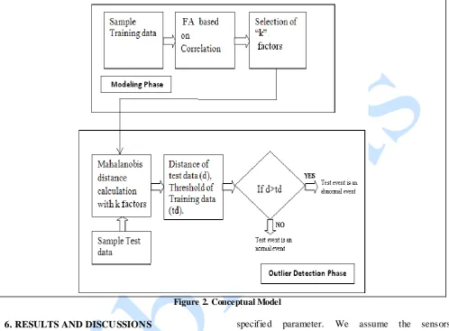
The conceptual model of the proposed system is illustrated in Figure 2. The algorithm is implemented in two phases: the data modeling phase, that creates a model of the normal condition of the monitored parameters, and the outlier detection phase, that
detects anomalies by comparing the actual data with the modeled one. During the data modeling phase, FA is applied on the correlation matrix of the sample data set and the first k most important factors are selected.
Figure 2. Conceptual Model
6. RESULTS AND DISCU SSIONS
This section specifies the performance evaluation of our technique compared to the PCA with subspace approach in [CP07] .We conduct experiments on the real data gathered from a deployment of WSN in the Intel Berkeley Research Laboratory [***]. The protocol is simulated in Matlab and considers a cluster as shown in Figure 3. The real data are collected from a closed neighbourhood from a WSN deployed in the Intel Berkeley Research Laboratory as shown in Figure 3. IBRL data set obtained from 54 sensor nodes, namely node ID from 1 to 54, during the four hours period collected on 1st March 2004 during the time interval 00:00am to 03:59am. We consider three features namely temperature, humidity and voltage. The closed neighbourhood contains the node 35 and its 5 spatially neighbouring nodes, namely nodes 1, 2, 3, 33, 35. The network recorded temperature, humidity, light and voltage measurements at 31 seconds intervals.
We consider a simulation setup, where N sensors are deployed over a particular region to monitor a
specified parameter. We assume the sensors communicate in multi-hop fashion. The sample was generated by multivariate dependency. We have kept as the number of compromised nodes at a time and as the corruption rate that defines the rate at which an adversary makes the data alteration.
Figure 3. Sensor nodes deployed in Intel Berkeley Research Lab
Figure 4. Factor Analysis Vs PCA approach
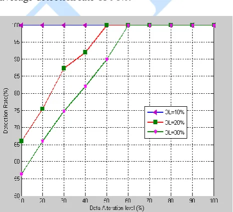
To obtain the model we have made 50 simulation runs for zero and . We evaluated the performance using two metrics namely detection rate and false alarm rate. Receiver Operating Characteristics (ROC) curve is used to visualize the tradeoff between the detection and false alarm rate. Figure 4 compares the detection rate of the factor analysis with mahalanobis distance to the PCA with subspace approach for multiple outliers. In Figure 4, the x-axis represents the faulty data rate and y-axis represents detection rate for different cluster size C. From Figure 4, we can see that Factor analysis based approach is effective in detecting the inconsistent data as the detection probability rapidly increases to a high value (90%). While PCA approach offer only an average of 85% detection rate. Figure 5 shows the detection rate of factor analysis for different data alteration rate in different outlier percentage OL for a fixed cluster size.
From the Figure 5, it is clear that it is effective in detecting outliers even when half of the cluster nodes in a cluster are faulty and found to maintain an average detection rate of 90%.
Figure 5. Detection rate for different outlier percentage
CONCLUSION
In this paper, we have proposed an outlier detection technique based on factor analysis and mahalanobis distance. Factor analysis describes the ordinary network behaviour by discovering the hidden structure of them. It also reduces large number of dataset into a smaller number of factors. The Mahalanobis distance is used to determine the “similarity” of network activities to the profiles. We compare the performance of our approach with the PCA and Subspace approach using real data of the Intel Berkeley Research Laboratory. Experimental research shows that our approach gives better performance for outlier data and does not require outlier free training data to design model. Based on comparative results that we obtained, we conclude that our proposed methodology improves significantly the anomaly detection capabilities, especially when compared against conventional principal component analysis based anomaly detection approach.
REFERENCES
[Aky02] I. F. Akyildiz et al. - Wireless Sensor
Networks: A Survey, Computer
Networks, vol. 38, no. 4, 2002, pp. 393– 422.
[AB06] Hair Anderson, Tatham Black -
Multivariate Data Analysis, Dorling
Kindersley, Pearson Education, 2006.
[BS07] S. Brown, C. J. Sreenan - A Study on Data Aggregation and Reliability in
Managing Wireless Sensor Networks”,
IEEE 2007.
[CES04] David Culler, Deborah Estrin, Mani Srivastava - Overview of Sensor
Network, IEEE 2004.
[CP07] Vassilis Chatzigiannakis, Symeon Papavassiliou - Diagnosing Anomalies and Identifying Faulty Nodes in Sensor
Networks, IEEE Sensors Journal,
VOL.7, NO.5, MAY 2007.
[C+06] V. Chatzigiannakis, S. Papavassiliou, M. Grammatikou, B. Maglaris - Hierarchical Anomaly Detection in
Distributed Large-scale Sensor
Networks, IEEE 2006.
In-Network Data Aggregation Scheme for
Wireless Sensor Network, in
International Journal of Futuristics Computer Applications, FCS Publisher, 25th February 2010
[C+10b] N. Chitradevi - Outlier aware Data Aggregation in Distributed Wireless Sensor Network using Robust Principal
Component Analysis, Selected for IEEE
sponsored International Conference ICCCN 2010, Chettinad College of Engineering and Technology, Karur, 31st May 2010.
[HCB00] W. R. Heinzelman, A. Chandrak asan, H. Balakrishnan - Energy-Efficient Communication Protocol for Wireless
Micro-sensor Networks, in the Hawaii
International Conference on System Science, Maui, Hawaii, 2000.
[JSF06] Xu Jianbo, Zeng Siliang, Qu Fengjiao
- A new In-network Data Aggregation
Technology of Wireless Sensor
Networks, IEEE 2006
[JW98] R. A. Johnson, D. W. Wichern -
Applied Multivariate Statistical
Analysis, Upper Saddle River, NJ :
Prentice Hall, 1998.
[Sze04] R. Szewczyk et al. - Habitat monitoring
with sensor networks, CACM, vol.47,
no.6, pp.34-40, 2004.
[TH05] S. Tanachaiwiwat, A. Helmy - Correlation analysis for alleviating effects of inserted data in wireless
sensor networks, in Proc. Mobile and
Ubiquitous Syst.: Networking Services , 2005, pp. 97– 108.
[WDA09] Mohamed Watfa, William Daher and Hisham Al Azar - A Sensor Network
Data Aggregation Technique,
International Journal of Computer Theory and Engineering Vol. 1, No. 1, April 2009