Evaluating a mesoscale atmosphere model and a satellite-based algorithm in estimating extreme rainfall events in northwestern Turkey

algorithm in estimating extreme rainfall events in

northwestern Turkey

I. Yucel and A. Onen

Department of Civil Engineering, Water Resources Lab, Middle East Technical University, Ankara, Turkey

Correspondence to: I. Yucel ([email protected])

Received: 30 September 2013 – Published in Nat. Hazards Earth Syst. Sci. Discuss.: 4 December 2013 Revised: 9 November 2013 – Accepted: 9 February 2014 – Published: 17 March 2014

Abstract. Quantitative precipitation estimates are obtained

with more uncertainty under the influence of changing cli-mate variability and complex topography from numerical weather prediction (NWP) models. On the other hand, hy-drologic model simulations depend heavily on the availabil-ity of reliable precipitation estimates. Difficulties in estimat-ing precipitation impose an important limitation on the pos-sibility and reliability of hydrologic forecasting and early warning systems. This study examines the performance of the Weather Research and Forecasting (WRF) model and the Multi Precipitation Estimates (MPE) algorithm in produc-ing the temporal and spatial characteristics of the number of extreme precipitation events observed in the western Black Sea region of Turkey. Precipitation derived from WRF model with and without the three-dimensional variational (3DVAR) data assimilation scheme and MPE algorithm at high spa-tial resolution (5 km) are compared with gauge precipita-tion. WRF-derived precipitation showed capabilities in cap-turing the timing of precipitation extremes and to some extent the spatial distribution and magnitude of the heavy rainfall events, whereas MPE showed relatively weak skills in these aspects. WRF skills in estimating such precipitation char-acteristics are enhanced with the application of the 3DVAR scheme. Direct impact of data assimilation on WRF precipi-tation reached up to 12 % and at some points there is a quan-titative match for heavy rainfall events, which are critical for hydrological forecasts.

1 Introduction

Influences of global warming and climate change are becom-ing more dominant with increasbecom-ing numbers of catastrophic events observed around the world. With global warming, ma-jor changes in rain and water cycles are being observed, fre-quency of meteorological disasters such as heavy rainfalls are increasing continuously, consequently resulting in high drought and flood risks. For example, the study of precipita-tion amounts during the last 50 years on land shows that the percentage of extreme precipitation compared to total precip-itation has increased (Trenberth et al., 2007). As it occurs and is evident in several geographical regions on the earth, these types of extreme events are also being observed throughout regions more prone to flooding in semiarid environments. Also, in regions having complex topography, extreme events show significant temporal and spatial variations and generate extensive amounts of precipitation in short durations.

forecasting has been a highly challenging task for more than half a century. Traditionally, weather forecasting has been based mainly on numerical weather prediction (NWP) mod-els and they are the most reliable source for atmospheric forecasts with a large spatial coverage and high temporal resolution (Liu et al., 1997). Mesoscale NWP models have played an important role in operational as well as severe weather forecasting. High-resolution mesoscale models can contribute to localized weather forecasting, particularly in ar-eas where the topography and land-use heterogeneity modu-late synoptic-scale weather. The verification studies of these mesoscale models, which are essential in terms of model pre-dictability, have been gaining interest in recent years. A num-ber of studies, such as those by Colle et al. (2003a, b), Kim and Lee (2006), Lin and Colle (2009), Shi et al. (2010), have verified the predictability of mesoscale models and gener-ally focused on quantitative precipitation forecasts/estimates (QPF/QPE) and evaluated various statistical techniques for improved QPF/QPE.

However, accurate precipitation calculations from NWP models are still a challenge. With appropriate initial and lateral-boundary conditions, high-resolution mesoscale mod-els offer great potential for improved QPF/QPE because models with this resolution can have skill in predicting the initiation and organizational mode of convective systems (Done et al., 2004). A study from Weisman et al. (1997) showed that 4 km grid spacing appears to be sufficient in resolving the dominant circulations in organized convective systems. NWP models provide an accessible tool for better understanding and improving the predictability of complex weather phenomena such as heavy rainfall events, while they are performed to add to the insufficient observational data for identifying extreme precipitation events. Because of the in-sufficient enforcement of initial- and boundary data to iden-tify storms, the initiation of mesoscale systems in real cases was difficult to simulate well (Choi et al., 2011). Therefore, many studies have suggested that data assimilation is a use-ful tool in order to improve the initial conditions for simu-lations (Liu et al., 2005; Yu, 2007; Choi et al., 2011) and the three-dimensional variational assimilation (3DVAR) has become a predominant method for providing initial model data in these studies and others (e.g., Lee et al., 2010). How-ever, the 3DVAR assimilation technique is yet to be success-fully applied for severe weather estimations, especially for the amount of heavy rainfall in Turkey. Therefore, it is im-perative to conduct mesoscale model tests and verify the re-sults to provide a direction for the improvement of model forecasts.

Heavy precipitation events are serious weather hazards in the eastern Mediterranean and Black Sea region. Although the number of previous studies (e.g., Borga et al., 2007; Nikolopoulos et al., 2013) focused on the prediction efforts of these rainfall events in the eastern Mediterranean, the stud-ies are significantly limited in Black Sea region. The Gen-eral Directorate of Meteorology (GDM) in Turkey uses its

operational NWP models over this region, but the verifica-tion studies of NWP results for heavy rainfall events ob-served in the western Black Sea region of Turkey have been lacking so far. Therefore, this study marks an effort to evalu-ate the Weather Research and Forecasting (WRF) model that is also being used as an operational model at the GDM. It includes a 3DVAR assimilation scheme for its performance and error statistics, notably in the western Black Sea region which experiences multiple flood threats, especially during spring and summer seasons. As a result, this study aims to improve the ability of the WRF model to estimate heavy-rain-producing systems and the associated QPE and evaluate the forecast impacts of the 3DVAR data assimilation system and the performance of mesoscale WRF model at 4 km res-olution. Nonconventional observations, such as meteorolog-ical satellites, provide additional and sufficient information for heavy rainfall events at high spatial (5 km) and tempo-ral resolution (15 min) and therefore, precipitation derived from the Multi-sensor Precipitation Estimates (MPE) algo-rithm (Heinemann et al., 2002) are also used in comparison when WRF model with and without assimilation is evaluated against observations.

2 Methodology

2.1 Study area and data

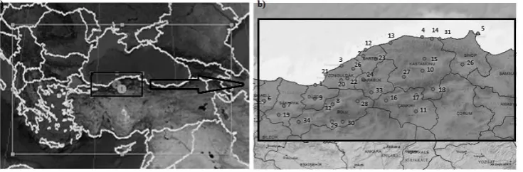
Fig. 1. The study area with WRF model configuration of two nested domains at 12 km and 4 km resolutions is shown in (a) and the detailed view of 4 km domain with the locations of rain gauge stations used in comparison as well as the border of city provinces in the region are shown in (b). Numbers 1 and 2, located at the center point of coarse- and fine-resolution domains, identify 12 km and 4 km domains, respectively.

Table 1. Studied events and their occurrence periods with the rainfall peak locations are given.

Event no. Start date End date Peak observation locations

1 02-06-00 07-06-00 Bartın

2 04-08-02 12-08-02 Kastamonu (Devrekani) 3 16-08-02 23-08-02 Kastamonu (Devrekani) 4 11-08-04 16-08-04 Zonguldak (Ere˘gli) 5 14-08-04 19-08-04 Bartın, Kastamonu 6 23-08-04 28-08-04 Bartın

7 28-04-05 05-05-05 Bartın, Bolu, Düzce 8 02-07-05 09-07-05 Bartın

9 13-07-05 18-07-05 Bartın, Zonguldak

10 05-06-07 15-06-07 Kastamonu (Cide), Zonguldak (Devrek) 11 30-07-07 04-08-07 Zonguldak

12 20-09-07 25-09-07 Zonguldak, Düzce (Akçakoca) 13 27-09-08 02-10-08 Kastamonu (˙Inebolu, Bozkurt) 14 12-07-09 17-07-09 Bartın, Kastamonu (Devrekani) 15 26-07-09 29-07-09 Kastamonu (Cide, ˙Inebolu) 16 06-09-09 12-09-09 Sakarya, Bolu

17 19-09-09 25-09-09 Bartın

18 25-06-10 02-07-10 Bartın, Bolu, Kastamonu (Devrekani) 19 06-07-10 11-07-10 Çankırı (Ilgaz), Bolu

20 31-08-10 04-09-10 Bartın 21 13-09-10 16-09-10 Bartın

22 01-10-10 04-10-10 Kastamonu (Bozkurt) 23 07-10-10 12-10-10 Bartın, Kastamonu (Bozkurt)

24 25-05-11 05-06-11 Kastamonu (Devrekani), Karabük (Yenice) 25 09-06-11 14-06-11 Bartın, Zonguldak (Ere˘gli, Devrek)

rainfall events and associated flood threats, especially dur-ing sprdur-ing and summer seasons. GDM develops the record of extraordinary meteorological events that occur through-out Turkey each year. As the main criteria, GDM considers any damage due to these events when selecting and record-ing. The number of heavy rain and associated flood events has been observed and marked in these records within this study region. According to these GDM records, the 25 spe-cific “heavy rain and flooding”-tagged hydrometeorological events between the years 2000 and 2011 are selected for this

Table 2. The name, elevation, latitude, and longitude of automated rain gauge stations of MGM used in this study.

Station

no. Station type Elevation (m) Latitude (◦) Longitude (◦) 1 Akcakoca 10.0 41.083 31.167 2 Bartin 33.0 41.633 32.333 3 Zonguldak 136.0 41.450 31.800 4 Inebolu 64.0 41.983 33.783

5 Sinop 32.0 42.033 35.167

6 Kocaeli 76.0 40.767 29.933 7 Sakarya 31.0 40.683 30.417

8 Bolu 743.0 40.733 31.600

9 Duzce 146.0 40.833 31.167 10 Kastamonu 800.0 41.367 33.783 11 Cankiri 751.0 40.617 33.617 12 Amasra 73.0 41.750 32.383

13 Cide 36.0 41.883 33.000

14 Bozkurt 167.0 41.950 34.017 15 Devrekani 1050.0 41.583 33.833 16 Cerkes 1126.0 40.817 32.900 17 Ilgaz 885.0 40.917 33.633 18 Tosya 870.0 41.017 34.033 19 Devrek 100.0 40.517 30.300 20 Acisu-radar 1112.0 41.181 31.799 21 Eregli 191.0 41.283 31.417 22 Geyve 100.0 41.217 31.950 23 Ulus 162.0 41.582 32.637 24 Yenice 140.0 41.200 32.333 25 Boyabat 350.0 41.467 34.767 26 Caycuma 50.0 41.400 32.083 27 Arac 650.0 41.250 33.333 28 Gerede 1270.0 40.800 32.200 29 Seben 757.0 40.417 31.583 30 Kıbriscik 1025.0 40.417 31.850 31 Catalzeytin 75.0 41.950 34.217 32 Boludagi 948.0 40.717 31.417 33 Eskipazar 757.0 40.967 32.533 34 Goynuk 780.0 40.400 30.783

can be found in the reference of Sönmez (2013). Quality con-trol tests applied to these rain gauge data are also described in this reference. When comparing the data between the WRF-and MPE-derived rainfall to rain gauges the point compari-son method is used, in which 4 km WRF and 5 km satellite pixels encompass each gauge measurement.

2.2 WRF modeling system

The Weather Research and Forecasting (WRF) model (Ska-marock et al., 2005) of mesoscale NWP system that incor-porates advanced numeric and data assimilation techniques (3DVAR), a multiple nesting capability, and numerous state-of-the-art physics options is suitable for extreme weather applications in this study. Development and verification of WRF have been carried out in many applications, including Lee et al. (2010) and Flesch and Reuter (2012), which are the most recent studies focused on heavy rainfall predictions at high spatial resolution. The WRF was employed in a nested configuration with grid points at 12 km and 4 km resolutions,

with its fine-sized domain covering the western Black Sea re-gion in the northwest of Turkey (see Fig. 1). The model was initiated, and time-varying lateral boundaries for the coarse domain then nudged every 3 h, using 25 km analysis fields from the European Centre for Medium-Range Weather Fore-casts (ECMWF). The WRF model is initiated at least a day earlier from the starting of the event to give the model some spin-up time. A high-resolution (30 s) data set was used to characterize modeled land surface across the fine-grid do-main, while the modeled atmosphere was described at 23 levels (up to level slightly higher than stratopause), these being stretched in the lower levels to ensure that resolu-tion in the boundary layer is adequate for use of the plane-tary boundary layer scheme. As the lowest boundary of the WRF model, Noah land surface model calculates the soil– vegetation–atmosphere interactions between surface and at-mosphere. Microphysical and cumulus schemes were kept active to calculate convective and non-convective precipita-tion processes on both domains. Convective tendencies are usually resolved within a 1- to 4 km grid scale and therefore the 4 km grid of model inner domain is found to be appro-priate in simulating heavy rainfall events in this study. Only precipitation from a fine-resolution domain at an hourly time step is used in analyses.

2.2.1 3DVAR setting

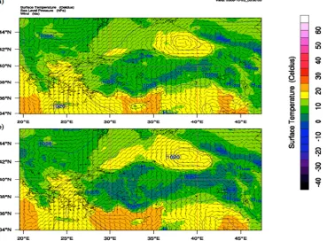
Fig. 2. The distribution of initial surface temperature, contours of sea level pressure and wind vectors for coarse domain on 25 October 2008 at 00:00 UTC (a) for WRF without assimilation (control) and (b) for WRF with assimilation.

with respect to new analyses, and model boundary conditions are updated. As an example, Fig. 2 shows the distribution of initial surface temperature, contours of sea level pressure and wind vectors for coarse domain on 25 October 2008 at 00:00 UTC in panel (a) for WRF without assimilation (con-trol), and in panel (b) for WRF with assimilation. The differ-ence in these fields is significantly traceable, hdiffer-ence the effect of assimilation becomes clear. Assimilation initial condition over land is colder, while over sea it is warmer and associated changes in wind and pressure are observable for this particu-lar case.

WRF model simulations with and without assimilation are performed for the duration of each event shown in Table 1. Hereafter, the control WRF simulation and the WRF simula-tion with a 3DVAR scheme will be referred to as WRF NOAS and WRF AS, respectively.

2.2.2 Parameterization testing

Several options for physics parameterizations that are ac-tual model representations of sub-grid scale processes are available in the WRF system. Note that only radiation, land surface and boundary layer physics in Table 3 were cho-sen as standards from available literature. The implemen-tation of various physics schemes, as well as their interac-tions, cause a large variation in the forecast output (Zhang et al., 2006), especially the choice of cumulus scheme and

microphysics. The particular skill of a cumulus and micro-physics scheme in simulating rainfall is dependent upon the region and storm being modeled (Giorgi and Mearns, 1999). Therefore, key parameterization of cumulus convection and microphysics in the WRF model was tested to yield an opti-mal configuration that would give reasonably good precipita-tion simulaprecipita-tion for heavy rainfall events. All these tests with WRF AS and WRF NOAS were performed on a particularly heavy rainfall event that was recorded on 12–17 July 2009, identified by event number 14 in Table 1. Table 3 lists the four combinations of cumulus and microphysics parameter-izations; namely “mp14cp1”, “mp2cp1”, “mp2cp5”, and

“mp14cp5” as well as other standard physics options

(radi-ation, land surface layer, and boundary layer) used in WRF model.

Fig. 3. Bias, RMSE, and false alarm rate (FAR) are shown in (a), (b), and (c), respectively, for different microphysics and cumulus options when WRF model is simulated with assimilation (AS) and without assimilation (NOAS) on 12–17 July 2009.

Table 3. Combinations of microphysics and cumulus parameterizations for optimal configuration as well as other physics used in the WRF model. mp and cp stand for microphysics and cumulus schemes, respectively, which are used with options 2 and 14 for mp and 1 and 5 for cp available in WRF model.

Combination mp14cp1 mp2cp1 mp2cp5 mp14cp5

Microphysics (mp) Lim and Hong (2010) Lin et al. (1983) Lin et al. (1983) Lim and Hong (2010) Cumulus (cp) Kain and Fritsch (1992) Kain and Fritsch (1992) Grell et al. (1995) Grell et al. (1995)

Radiation Dudhia (1989) Dudhia (1989) Dudhia (1989) Dudhia (1989)

Land surface layer Chen and Dudhia (2001) Chen and Dudhia (2001) Chen and Dudhia (2001) Chen and Dudhia (2001) Boundary layer Hong and Pan (1996) Hong and Pan (1996) Hong and Pan (1996) Hong and Pan (1996)

sensitivity is to the choice of convective treatment rather than microphysics. On the other hand, WRF skill is improved with AS according to statistics between AS and NOAS. After test-ing the combinations of these schemes, the resulttest-ing optimal physics configuration is Lim and Hong (2010) (microphysics scheme) and Kain and Fritsch (1992) (cumulus convection).

2.3 Satellite rainfall algorithm

The MPE is an instantaneous rain-rate product, which is de-rived from 10.7 µm brightness temperatures of Infrared (IR)-data of geo-stationary EUMETSAT satellites by continuous recalibration of the algorithm with rain-rate data from po-lar orbiting microwave sensors (Heinemann et al., 2002). The MPE provides precipitation data with high spatial res-olution at 3 km at sub-satellite points and 5 km in the study area, while temporal resolution is 15 min. The algorithm provides better results in convective cases than the strati-form cases. Frontal precipitation, especially at warm fronts is very often wrongly located and overestimated. MPE data in this study are obtained from GDM for the whole disc area (3712×3712) in a 15 min period for heavy rainfall events ob-served after 2005 in Table 1. Since comparison analyses are performed in hourly time intervals, the hourly MPE amounts are obtained by aggregating the four 15 min instantaneous rain rates within an hour.

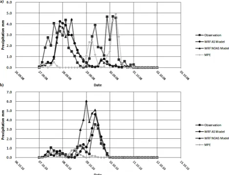
Fig. 4. Area-averaged time series of WRF AS, WRF NOAS, and MPE against observations are shown in (a) for event number 13 and (b) for event number 23.

3 Results

3.1 General analyses

Fig. 5. Scatter diagrams of all data at 3 h intervals are shown in (a) between WRF with assimilation and observation, (b) between WRF without assimilation and observation, and (c) between MPE and observation.

WRF model better follows observed temporal fluctuations than non-assimilated WRF and MPE, except during the sec-ond peak of rainfall event 13, where MPE is in agreement with the ground observation. Assimilation provided a very good match with observation for event 23 by reducing the rainfall amount produced by WRF NOAS in the late after-noon of 9 October 2010 in Fig. 4b. However, MPE com-pletely misses the peak of this event. The scatter analyses of WRF AS/NOAS and MPE against observations using data from all 25 rainfall events are performed in order to inspect their degree of association. The levels of scattering between data pairs as well as overestimation and underestimation ten-dencies against observations are determined from these anal-yses. Figure 5 shows the scatter plots in panel (a) between WRF AS and observation, panel (b) between WRF NOAS and observation, and panel (c) between MPE and observa-tion for 3-hourly rainfalls. The linear trend lines of data pairs are also shown in this figure. WRF AS shows less scatter than WRF NOAS, hence it produces a better degree of as-sociation with observation. Compared to WRF AS, a some-what higher level of scattering is inspected in WRF NOAS that is mainly attributed to extreme overestimation and un-derestimation data points tends to be modified by WRF AS through data assimilation. MPE gives slightly higher corre-lation values than WRF with and without assimicorre-lation as it releases less extreme rainfall amounts and tends to underes-timate heavy rainfall events.

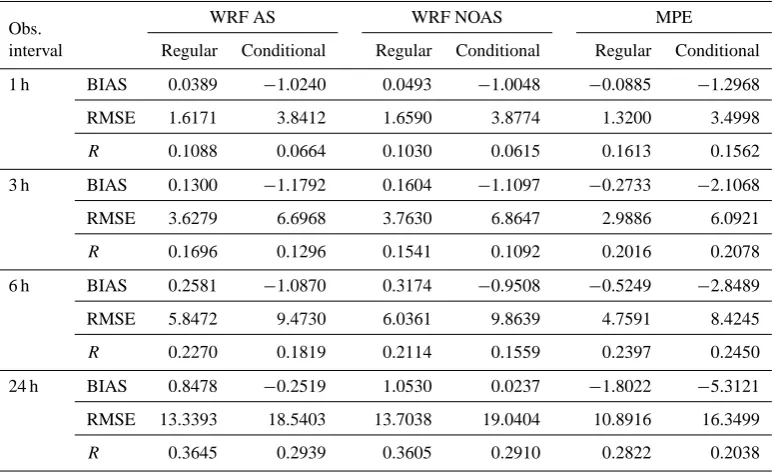
RMSE, bias and correlation coefficient (R) of WRF AS, WRF NOAS and MPE are calculated for 1-, 3-, 6-, and 24-hourly rainfalls and the results with regular and conditional precipitation (only non-zero observed precipitation cases) are given in Table 4. According to results, the assimilation shows a consistent improvement on WRF precipitation at all time intervals. With WRF AS the lower RMSE, bias values and higher correlation coefficients compared to WRF NOAS are obtained. Correlation coefficients increase with increasing time intervals from 1 to 24 h. Negative biases at all time inter-vals with MPE indicate persistent underestimation features in regular and conditional rains and this feature becomes more significant than latter. However, WRF with and without data assimilation shows the underestimation only with conditional

rain. When compared to the WRF model, MPE shows better statistics in 1-, 3-, and 6-hourly rains but it shows a lower correlation than WRF for daily rains because of a more pro-nounced effect of high negative biases at this interval. It should be pointed out that the lower RMSE values with MPE are largely due to lower average rainfall intensity and are not necessarily indicative of greater accuracy. With conditional rains, statistical performances of WRF and MPE decrease further with higher RMSE and biases, and lower correla-tion when only observed rainy periods are considered. Higher negative biases with conditional rains of the WRF model in-dicate the fact that assimilation generally tends to reduce the precipitation amount in WRF. Across the study area, the er-ror is reduced by 2.53 % in 1 h, 3.59 % in 3 h, 3.13 % in 6 h, and 2.66 % in 24 h intervals with regular rain analysis and by 0.94 % in 1 h, 2.45 % in 3 h, 3.96 % in 6 h, and 2.63 % in 24 h intervals with conditional rain analysis with the addition of the 3DVAR scheme in the WRF model. Precipitation with 3 h interval in regular analysis and 6 h interval in conditional analysis showed the highest improvement.

The skills of the WRF and MPE algorithm are evaluated further by calculating the equitable threat score (ETS) and its bias (ETS Bias) for daily rainfall as functions of different daily precipitation threshold values.

These scores are defined (Lee et al., 2004) as follows: ETS=(A−H )/(A+B+C−H ),

H=(A+B)(A+C)/(A+B+C+D),

ETS Bias=(A+B)/(A+C),

Table 4. Bias and RMSE in [mm] and correlation coefficient (R) of WRF AS, WRF NOAS, and MPE for regular and conditional rain amounts at 1, 3, 6 and 24 h intervals are given. Conditional rain represents only non-zero observed precipitation cases.

Obs. WRF AS WRF NOAS MPE

interval Regular Conditional Regular Conditional Regular Conditional

1 h BIAS 0.0389 −1.0240 0.0493 −1.0048 −0.0885 −1.2968

RMSE 1.6171 3.8412 1.6590 3.8774 1.3200 3.4998

R 0.1088 0.0664 0.1030 0.0615 0.1613 0.1562

3 h BIAS 0.1300 −1.1792 0.1604 −1.1097 −0.2733 −2.1068

RMSE 3.6279 6.6968 3.7630 6.8647 2.9886 6.0921

R 0.1696 0.1296 0.1541 0.1092 0.2016 0.2078

6 h BIAS 0.2581 −1.0870 0.3174 −0.9508 −0.5249 −2.8489

RMSE 5.8472 9.4730 6.0361 9.8639 4.7591 8.4245

R 0.2270 0.1819 0.2114 0.1559 0.2397 0.2450

24 h BIAS 0.8478 −0.2519 1.0530 0.0237 −1.8022 −5.3121

RMSE 13.3393 18.5403 13.7038 19.0404 10.8916 16.3499

R 0.3645 0.2939 0.3605 0.2910 0.2822 0.2038

WRF AS, WRF NOAS, and MPE are shown, respectively, in Fig. 6a and b for different daily precipitation threshold values. In Fig. 6a, there is a more gradual decrease in ETS scores of WRF AS and NOAS than decrease in those of MPE along with increasing precipitation thresholds. MPE does not produce any score after an approximate thresh-old value of 48 mm day−1. Significant discrepancy between WRF AS/NOAS and MPE scores after about a 3 mm day−1 threshold value explains that MPE shows a roughly 10 % lower performance than the WRF model on capturing daily precipitation thresholds. WRF AS and NOAS show a steady increase in ETS Bias after a threshold value of 15 mm day−1, while MPE shows a gradual but continuous decrease in ETS Bias along with threshold range in Fig. 6b. In addition, ETS Bias values with the WRF always stay above 1, while those with MPE always stay far below 1. It is notable that the over-estimation feature of WRF increases gradually up to 40 %, while the underestimation feature of MPE increases up to 90 % towards higher precipitation thresholds. These behav-iors in WRF and MPE consequently cause a decreasing trend in ETS with increased precipitation thresholds. On the other hand, for both of these skill measures, WRF AS consis-tently produced better skills than WRF NOAS almost at all threshold values, while both WRF (AS and NOAS) scores (ETS and ETS Bias) yielded much better performance than MPE. The substantial underestimation feature of MPE al-ready given in Table 4 is consistent with these score analyses of different precipitation thresholds.

Fig. 6. ETS and ETS Bias scores of WRF AS, WRF NOAS, and MPE are shown, respectively, in (a) and (b) for different daily pre-cipitation threshold values.

3.2 Event- and station-based analyses

Fig. 7. Bias, RMSE, and correlation coefficient (R) of WRF AS, WRF NOAS, and MPE at 3 h interval are shown in (a) for each event and (b) for each station.

RMSE and increase in R are observed on WRF AS with respect to WRF NOAS, while a majority of events (87 %; 13 out of 15 events) and stations (71 %; 24 out of 34 sta-tions) shows significant negative biases with MPE as this was the case in previous analyses. The dry bias character of MPE results in falsely lower RMSE compared to the WRF in many cases but the correlation coefficient or general pat-tern of MPE yields better skill than the WRF with and with-out assimilation in 44 % of the events and 41 % of the sta-tions. On the other hand, WRF AS yields better performance than WRF NOAS in 60 % of the events (15 out of 25 events) and 70 % of the stations (24 out of 34 stations) based on root mean squared errors, and in 72 % of the events (18 out of 25 events) and 79 % of the stations (27 out of 34 sta-tions) based on correlation coefficient values. Improvement with data assimilation is more evident in station-based anal-yses than that in event-based analanal-yses, and thereby the tem-poral effects are better interpreted than spatial effects with

assimilation within the WRF. This can be attributed to the greater uncertainty of spatial effects than temporal effects, as the study covers mostly summertime convective precipitation events. Furthermore, in both event- and station-based anal-yses, the correlation coefficient inspection releases higher number and more traceable improvement with assimilation than root mean squared error. This is an indication of high impact of assimilation on the track of a precipitation pattern rather than its magnitude.

Table 6. Error improvements in [%] with the use of 3DVAR in WRF are given at 1 h, 3 h, 6 h, and 24 h intervals for event- and station-based analyses. These improvements are provided for all data and partial data after excluding chaotic values with data assimilation.

Hourly time period

Analysis type Data type 1-hourly 3-hourly 6-hourly 24-hourly

Event-based All 4.31 5.13 3.72 4.21

Analysis Excluding chaotic values 7.80 9.19 9.29 10.12

Station-based All 2.79 4.29 3.81 4.08

Analysis Excluding chaotic values 8.99 11.39 11.46 11.20

parameterizing convective activities, hence they yield poor skill for precipitation resulting from convective types of sys-tems. However, this situation is reversed with the MPE, as its rainfall character shows great variability inter events per station. To point out the impact of assimilation on the WRF-derived precipitation amount, the mean error reduction rate or improvement rate in precipitation is computed for both event- and station-based analyses at each rainfall interval, and their results are shown in Table 6. In both event- and station-based analyses, 3-hourly rain intervals showed the highest improvement rates, with 5.13 % in event-based and 4.29 % in station-based when data assimilation is used in the WRF model. In some cases, shown in Fig. 7a and b, the assimilation degrades precipitation against observations be-cause of the chaotic processes available in the model. These processes, influenced by boundary conditions in the model, destroy the agreement between modeled and observed fields after data assimilation. These cases showed better agreement with observed rainfall when WRF was used without data as-similation. By excluding such cases from error analyses, the direct impact of assimilation on precipitation is more isolated and it enhances the error reduction rates further, as seen in Table 6. In this case, for example, the mean improvement rate is increased up to 11.39 % for 3 h intervals. Liu et al. (2013) showed the impact of 3DVAR with 16 % improvement on a 10 km single grid of 24 h accumulative rainfall when they used WRF with 3DVAR and traditional meteorological ob-servations at the initial state to simulate a rainfall storm.

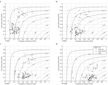
While the improvements provided by assimilation were given per event and per station basis in previous analy-ses, probability of detection (POD), FAR, and critical suc-cess index (CSI) values (Kidd et al., 2011) are evaluated to-gether to trace the change in precipitation performance of WRF with and without assimilation and MPE. For example, Fig. 8 shows these score values in panel (a) for 1 h inter-vals, panel (b) for 3 h interinter-vals, panel (c) for 6 h interinter-vals, and panel (d) for 24 h intervals for each of the 25 events, while Fig. 9a, b, c, and d show the equivalent diagrams for each of the 34 stations. As both event and station charts, along with 1- to 24-hourly intervals, are examined in these figures, the MPE shows substantially higher FAR, slightly higher POD and lower CSI than those of the WRF model at all time

intervals. Also, as the time interval aggregates from 1 h to 24 h, the desired pattern of significant increase in POD and decrease in FAR is witnessed. Thus, the CSI value, which is a function of both POD and FAR, converges towards 1, shown within contours. FAR is the least improved parameter of MPE, along with time intervals, and this finding confirms the existence of a systematic problem in MPE that makes the algorithm persistently underestimate precipitation. In Fig. 8, a few stations show consistently low FAR values at all inter-vals in contrast to the rest of the stations with MPE, as the algorithm shows some ability to capture the track of storms from different events at these stations. Inter-event variability (see Fig. 8) on these statistical parameters is much more evi-dent than the variability appears among stations (see Fig. 9).

4 Summary and conclusions

In this study, QPE from the MPE rainfall algorithm and WRF model with and without data assimilation were evaluated against the network of 34 rain gauges installed in the par-tially mountainous region of the western Black Sea in Turkey during 25 different spring/summer/fall heavy rainfall event periods selected from 2000 to 2011. The study provides a comprehensive validation of the characteristics of WRF- and satellite-estimated precipitation to examine their abilities to accurately reproduce heavy rainfall events. In an effort to fur-ther improve the developed QPF by WRF model, the WRF model was also applied with a 3DVAR data assimilation scheme, and its potential in producing QPF for heavy rainfall events and for flood forecasting purposes was shown. Com-parisons indicate a promising potential of the WRF model in producing heavy rainfall events and with the use of data assimilation in WRF, the results are further improved with a better model performance. However, with an MPE algo-rithm some systematic bias structures exist that need to be addressed. The primary conclusions of the present research are summarized as follows:

– The Kain–Fritsch cumulus and The Lim and Hong

Fig. 8. POD, FAR and CSI statistics of WRF AS, WRF NOAS and MPE are shown together for each of the 25 events at 1, 3, 6, and 24 h intervals in (a), (b), (c), and (d), respectively. Contours represent CSI values.

for both assimilation and no assimilation. Also, pre-cipitation is found to be most sensitive to the cumu-lus scheme rather than the microphysics scheme, ac-cording to experimental design of determining the op-timum parameterization in WRF, as this agrees with the results of Lowrey and Yang (2008).

– Overall, the WRF model with and without

assimila-tion generates an overestimaassimila-tion trend against observa-tions, while MPE substantially underestimates the pre-cipitation. However, when only conditional rains are considered WRF model also shows some underestima-tion.

– On mean areal time series, assimilated WRF model

especially managed to match temporal observation trends and rain amounts up to some extent. While tem-poral consistence shows variance for each event, in some events this consistency is observed much more significantly. The MPE manages weakly to match dense local rain gradients observed on WRF because of its underestimation behavior.

– WRF with assimilation greatly improved precipitation

with respect to no assimilation at all time intervals and the improvement was the highest with 3-hourly pre-cipitation. Error statistics shows that across the net-work, the assimilation improved the rainfall by 4 % in various time intervals, but mostly over the 3 h in-terval for regular and conditional rainfall. Assimila-tion tends to trim the precipitaAssimila-tion amount in WRF according to the area-averaged conditional rain anal-yses across the events. WRF with and without assim-ilation showed substantially better performance than MPE with threshold analysis while AS yielded better skill than NOAS at almost all threshold values.

– Improvement of data assimilation was more evident

in station-based analyses than event-based analyses, whereas MPE acted reversely by releasing smaller mean error in event-based analysis. For both analyses, the 3-hourly mean error is reduced roughly by about 5 % with data assimilation, and when the chaotic cases are not included in analyses, the mean error reduction rate is improved to 10 % for event-based and 12 % for station-based analyses. Assimilation shows a tendency of higher impact on precipitation trend than its magni-tude.

– Time aggregation from 1- to 24 h make the POD, FAR

and CSI converge towards their high success values. In both event- and station-based charts, MPE values show overwhelmingly higher FAR and somewhat lower CSI trends, while showing POD values close to WRFs; this feature persists at all time intervals. Mean variability among stations is clearly less than among events ac-cording to POD, FAR, CSI combinations.

The study showed that WRF was often able to detect heavy rainfall signals based on 25 events. Though it may not sim-ulate both the occurrence time and the rainfall magnitudes accurately, it manages to simulate them satisfactorily. Data assimilation has a significant role in this satisfactory perfor-mance of WRF systems. In addition, as a beneficiary point of data assimilation used in this study, Liu et al. (2013) found that obvious improvement can be observed regarding both the rainfall cumulative curve and the 24 h rainfall total af-ter assimilating the traditional observations via 3DVAR in WRF. They also stated the improvement of radar data assim-ilation through 3DVAR is negligibly small when compared with the assimilation of the traditional meteorological obser-vations. The local-scale improvement of convective storms, which is apparently provided by data assimilation in this study, benefits flood warning issues performed at fine-scale locations. The capability of modeling systems is quite cru-cial, particularly as an advisory tool, for taking flood early warning measures. The heavy rainfall signals could be de-tected well in advance by WRF, which is very useful for flood advisory, particularly for locations showing very short hydrologic response times for the heavy rain events. On the other hand, although the MPE provides realistic precipita-tion in a few cases and is a good supplement for WRF, it requires modifications for its substantial underestimation be-havior that was mostly evident in this study. Contrary to this, for example, the operational hydro estimator (HE) rainfall algorithm of the National Oceanic and Atmospheric Admin-istration (NOAA), which is infrared-based algorithm similar to MPE, shows a tendency to overestimate precipitation with heavy rainfall events occurring during larger, more organized convective storms (Yucel et al., 2011). Perhaps the bias struc-ture suggests that the MPE may have a decreased sensitivity to deep convection, which weakly generates heavy precipi-tation in many events in this study. Also, it is suggested that the calibration equation that is used to modify IR-based rain-fall estimates with microwave data requires tuning in MPE algorithm.

Acknowledgements. This study is supported by European

pro-cedures for flood frequency estimation (FloodFreq) Cost Action (ES0901) and Tübitak ArdebÇaydag Scientific and Technological Research Project Program (1001) with Project no. 110Y036. Our special thanks to GDM staff, Mr. Ismail Mert for his continuous support on WRF simulations and rain gauge data acquisition process.

Edited by: A. Loukas

mesoscale convective systems accompanying heavy rainfall: the Goyang case, Asia-Pacific, J. Atmos. Sci., 47, 265–279, 2011. Colle, B., Olson, J. B., and Tongue, J. S.: Multiseason verification

of the MM5, Part I: Comparison with the Eta model over the central and eastern United States and impact of MM5 resolution, Weather Forecast., 18, 431–457, 2003a.

Colle, B., Olson, J. B., and Tongue, J. S.: Multiseason verification of the MM5, Part II: Evaluation of high-resolution precipitation forecasts over the northeastern United States, Weather Forecast., 18, 458–480, 2003b.

Done, J., Davis, C. A., and Weisman, M. L.: The next generation of NWP: explicit forecasts of convection using the Weather Re-search and Forecasting (WRF) model, Atmos. Sci. Lett., 5, 110– 117, 2004.

Dudhia, J.: Numerical study of convection observed during the winter monsoon experiment using a mesoscale two-dimensional model, J. Atmos. Sci., 46, 3077–3107, 1989.

Giorgi, F. and Mearns, L. O.: Introduction to special section: re-gional climate modeling revisited, J. Geophys. Res., 104, 6335– 6352, 1999.

Grell, G. A., Dudhia, J., and Stauffer, D. R.: A description of the fifth generation Penn State/NCAR mesoscale model (MM5), NCAR Tech. Note NCAR/TN-398+STR, 138 pp., Boulder, Col-orado, US, 1995.

Flesch, T. K. and Reuter, G.: WRF model simulation of two Alberta flooding events and the impact of topography, J. Hydrometeorol., 13, 695–708, 2012.

Heinemann, T., Lattenzio, A., and Roveda, F.: The Eumetsat Multi Sensor Precipitation Estimate (MPE), Eumetsat, Darmstadt, Ger-many, 2002.

Hong, S.-Y. and Pan, H.-L.: Nonlocal boundary layer vertical diffu-sion in a medium-range forecast model, Mon. Weather Rev., 124, 2322–2339, 1996.

Kain, J. S. and Fritsch, J. M.: Convective parameterization for mesoscale models: the Kain–Fritsch scheme, in: The Represen-tation of Cumulus Convection in Numerical Models, Meteor. Monogr., Am. Meteorol. Soc., 46, 165–170, 1992.

Kidd, C., Bauer, P., Turk, J., Huffman, G. J., Joyce, R., Hsu, K.-L., and Braithwaite, D.: Inter-comparison of high-resolution precip-itation products over northwest Europe, J. Hydrometeorol., 13, 67–83, 2011.

Kim. H.-W. and Lee, D.-K.: An observational study of mesoscale convective systems with heavy rainfall over the Korean penin-sula, Weather Forecast., 21, 125–148, 2006.

Lee, D.-K., Eom, D.-Y., Kim, J.-W., and Lee, J.-B.: High resolution rainfall prediction in the JHWC real-time WRF system, Asia-Pacific J. Atmos. Sci., 46, 341–353, 2010.

Lee, S., Lee, D., and Chang, D.: Impact of Horizontal Resolu-tion and Cumulus ParameterizaResolu-tion Scheme on the SimulaResolu-tion of

Research and Forecasting model, Mon. Weather Rev., 137, 1372– 1392, 2009.

Lin, Y.-L., Farley, R. D., and Orville, H. D.: Bulk parameterization of the snow field in a cloud model, J. Climate Appl. Meteor., 22, 1065–1092, 1983.

Liu, J., Bray, M., and Han, D.: A study on WRF radar data assimila-tion for hydrological rainfall predicassimila-tion, Hydrol. Earth Syst. Sci., 17, 3095–3110, doi:10.5194/hess-17-3095-2013, 2013. Liu, Y., Zhang, D.-L., and Yau, M. K.: A multiscale numerical study

of hurricane Andrew (1992), Part I: Explicit simulation and ver-ification, Mon. Weather Rev., 125, 3073–3093, 1997.

Liu, Y., Bourgeois, A., Warner, T., Swerdlin, S., and Hacker, J.: An implementation of observation nudging-based FDDA into WRF for supporting ATEC test operations, 2005 WRF user workshop, Boulder, Colorado, US, Paper 10.7, 2005.

Lowrey, M. R. K. and Yang, Z.-L.: Assessing the capability of a regional-scale weather model to simulate extreme precipitation patterns and flooding in Central Texas, Weather Forecast., 23, 1102–1126, 2008.

Nikolopoulos, E. I., Anagnostou, E. N., and Borga, M.: Using high-resolution satellite rainfall products to simulate a major flash flood event in northern Italy, J. Hydrometeorol., 14, 171–185, 2013.

Parrish, D. F. and Derber, J. C.: The National Meteorological Center’s spectral statistical interpolation analysis system, Mon. Weather Rev., 120, 1747–1763, 1992.

Sensoy, S., Demircan, M., Ulupinar, U., and Balta, I: Climate of Turkey, MGM Web address, available at: http://www.mgm. gov.tr/files/en-US/climateofturkey.pdf (last access: 25 Novem-ber 2013), 2008.

Shi, J. J., Tao, W.-K., Matsui, T., Cifelli, R., Hou, A., Lang, S., Tokay, A., Wang, N.-Y., Peters-Lidard, C., Skofronick-Jackson, G., Rutledge, S., and Petersen, W.: WRF simulations of the 20– 22 January 2007 snow events over eastern Canada: comparison with in-situ and satellite observations, J. Appl. Meteorol. Clim., 49, 2246–2266, 2010.

Skamarock, W. C., Klemp, J. B., Dudhia, J., Gill, D. O., Barker, D. M., Wang, W., and Powers, J. G.: A description of the Advanced Research WRF Version 2. Tech. rep., NCAR, Boulder, Colorado, US, 2005.

Sönmez, I: Quality control tests for western Turkey Mesonet, Me-teorol. Appl., 20, 330–337, doi:10.1002/met.1286, 2013. Trenberth, K. E., Jones, P. D., Ambenje, P., Bojariu, R., Easterling,

Weisman, M. L., Skamarock, W. C., and Klemp, J. B.: The resolu-tion dependence of explicitly modeled convective systems, Mon. Weather Rev., 125, 527–548, 1997.

Yu, W., Liu, Y., and Warner, T.: An evaluation of 3-DVAR, nudging-based fdda and a hybrid scheme for summer convection forecast using WRF-ARW model, 2007 WRF user workshop, Paper 2.4, Boulder, Colorado, US, 2007.

Yucel, I., Kuligowski, R. J., and Gochis, D. J.: Evaluating the hydro-estimator satellite rainfall algorithm over a mountainous region, Int. J. Remote Sens., 32, 7315–7342, 2011.