A Sharper Ratio

(1)

University of Pennsylvania

ScholarlyCommons

Publicly Accessible Penn Dissertations

1-1-2013

A Sharper Ratio

Xingtan Zhang

University of Pennsylvania, xingtan@sas.upenn.edu

Follow this and additional works at:http://repository.upenn.edu/edissertations

Part of theApplied Mathematics Commons

This paper is posted at ScholarlyCommons.http://repository.upenn.edu/edissertations/951

For more information, please contactlibraryrepository@pobox.upenn.edu. Recommended Citation

Zhang, Xingtan, "A Sharper Ratio" (2013).Publicly Accessible Penn Dissertations. 951.

(2)

A Sharper Ratio

Abstract

The Sharpe ratio is the dominant measure for ranking risky assets

and funds. This paper derives a generalized ranking measure which,

under a regularity condition, is valid in the presence of a much broader

assumption (utility, probability) space yet still preserves wealth

separation for the broad HARA utility class. Our ranking measure,

therefore, can be used with ``fat tails'' as well as multi-asset

class portfolio optimization. We also explore the foundations of asset

ranking, including proving a key impossibility theorem: any ranking

measure that is valid at non-Normal ``higher moments'' cannot generically

be free from investor preferences. Finally, we derive a closed-form

approximate measure (that can be used without numerical analysis),

which nests some previous attempts to include higher moments. Despite

the added convenience, we demonstrate that approximation measures

are unreliable even with an infinite number of higher moments.

Degree Type

Dissertation

Degree Name

Doctor of Philosophy (PhD)

Graduate Group

Applied Mathematics

First Advisor

Kent Smetters

Keywords

(3)

Subject Categories

(4)

A SHARPER RATIO

Xingtan Zhang

A DISSERTATION

in

Applied Mathematics and Computational Science

Presented to the Faculties of the University of Pennsylvania in Partial

Fulfillment of the Requirements for the Degree of Doctor of Philosophy

2013

Kent Smetters

Boettner Professor of Business Economics and Public Policy

Supervisor of Dissertation

Charles Epstein

Thomas A. Scott Professor of Mathematics

Graduate Group Chairperson

Robin Pemantle, Merriam Term Professor of Mathematics

(5)

Dedication

To my parents, for all the love and encouragement.

(6)

Acknowledgments

My deepest gratitude is to Dr. Kent Smetters for the continuous support of my

research, for his patience, encouragement, motivation and enthusiasm.

I would like to thank all my committee members: Dr. Robin Pemantle, Dr. Amir

Yaron and Dr. Domenico Cuoco for their insightful comments and encouragement.

I would also like to thank the graduate group in applied mathematics and

com-putational science, especially Dr. Charles Epstein for the support of my graduate

study and his patience, motivation and understanding.

Many friends have helped me through these years. I greatly value their friendship

and I deeply appreciate their belief in me.

Finally, and most importantly, I want to thank my wife Fan, my parents and

(7)

ABSTRACT

A SHARPER RATIO

Xingtan Zhang

Kent Smetters

The Sharpe ratio is the dominant measure for ranking risky assets and funds.

This paper derives a generalized ranking measure which, under a regularity

con-dition, is valid in the presence of a much broader assumption (utility, probability)

space yet still preserves wealth separation for the broad HARA utility class. Our

ranking measure, therefore, can be used with “fat tails” as well as multi-asset class

portfolio optimization. We also explore the foundations of asset ranking,

includ-ing provinclud-ing a key impossibility theorem: any rankinclud-ing measure that is valid at

non-Normal “higher moments” cannot generically be free from investor preferences.

Finally, we derive a closed-form approximate measure (that can be used without

nu-merical analysis), which nests some previous attempts to include higher moments.

Despite the added convenience, we demonstrate that approximation measures are

(8)

Chapter 1 Introduction

Sharpe (1966) demonstrated that picking a portfolio with the largest expected risk

premium relative to its standard deviation is equivalent to picking the portfolio that

maximizes the original investor’s expected utility problem, assuming that portfolio

returns are Normally distributed.1 _{The Sharpe ratio, therefore, is a convenient}

“sufficient statistic” for the investor’s problem since it does not rely on the investor’s

preferences or level of wealth.

The immense power of the Sharpe ratio stems from the fact that it allows the

investment management process to be decoupled from the specific attributes of the

heterogeneous investor base. Indeed, the multi-trillion dollar money management

(mutual fund and hedge fund) industry relies heavily on this separation. While

investors in a fund might differ in their risk aversion and level of wealth (including

(11)

outside assets), an investment manager only needs to correctly estimate the first

two moments of the Normal distribution that characterizes the fund’s risk.2 It is not

surprising, therefore, that the Sharpe ratio is tightly integrated into the investment

management practice and embedded into virtually all institutional investment

ana-lytics and trading platforms. Even consumer-facing investment websites like Google

Finance reports the Sharpe ratio for most mutual funds along with just a few other

basic statistics, including the fund’s alpha, beta, expected return, R2 _{tracking (if}

an indexed fund), and standard deviation.

Of course, it is well known that investment returns often exhibit “higher

or-der” moments that might differ from Normality (Fama 1965; Brooks and Kat 2002;

Agarwal and Naik 2004, and Malkiel and Saha 2005).3 In practice, investment

professionals, therefore, often look for investment opportunities that would have

historically – that is, in a “back test” – produced unusually large Sharpe ratios

under the belief that an extra large value provides some “buffer” in case the

under-2_{The Sharpe ratio, however, only ranks the various}_risky _{portfolios in the presence of a risk-free}

numeraire instrument. It does not determine the optimal split between the risky asset and the

risk-free asset, which must be determined in the second stage using consumer preferences. This

two-step process is generally known as “two fund separation.” Hence, there is still a role for

“personalized financial advice” in the Sharpe world and the need to understanding an investors

tolerance to risk.

3_{A related literature has examined how disaster risk can explain equilibrium pricing within}

the neoclassical growth model (Barro 2006, 2009; Gabaix 2008, 2012; Gourio 2012; and, Wachter

(12)

lying distribution is not Normal. Academic researchers, however, know that this

convention is often a mistake. A large Sharpe ratio often does not provide much

information outside of the assumption (utility, probability) space where the Sharpe

ratio is valid. Indeed, it is easy to create portfolios with large Sharpe ratios that

are actually first-order stochastically dominated by portfolios with smaller Sharpe

ratios.4 _{Multi-asset class portfolios with bonds, derivatives, and other securities}

of-ten produce left skewed distributions even if the if the core equity risk is Normally

distributed (Leland 1999; Spurgin 2001; and Ingersoll et al. 2007).5

The potential limits of the Sharpe ratio to correctly rank risky portfolios has

led to an interest in producing risk measures that take into account non-Normal

“higher-order” distribution moments. This literature dates back to at least the

early work by Paul Samuelson (1970). A short list of other contributors include the

seminal paper by Kraus and Litzenberger (1976), Scott and Horvath (1980), Owen

and Rabinovitch (1983), Brandt et al (2005), Jurczendo and Maillet (2006),

Za-kamouline and Koekebakker (2008), Dvila (2010) and Pierro and Mosevich (2011).

Much of this important work has extended Sharpe’s mean-variance ranking measure

to some additional moments of the risk distribution, typically under some

restric-4_{In other words, the portfolio with the smaller Sharpe ratio should be preferred by all expected}

utility maximizers with positive marginal utility in wealth.

5_{Ingersoll et al. (2007) also examine the potential of manipulation of returns by managers}

according to a criterion that they outline. In contrast, our focus is on how to rank risky investments

(13)

tions on preferences or some other mathematical simplifications. A second area of

research bypasses the investor’s expected utility problem altogether and instead

fo-cuses on producing risk measures that satisfy certain mathematical properties such

as “coherence.”6 _{Examples of coherent risk measures include “average VaR,”}

“en-tropic VaR,” and “super-hedging.” While these measures satisfy certain axioms, a

portfolio that best maximizes one or more of these measures does not necessarily

maximize the investor’s expected utility (i.e., the standard investor problem). A

third line of work has evolved, often from practitioners, and has produced more

heuristic measures including “value at risk (VaR),”7 _{Omega, Sortino ratio, Treynor}

ratio, Jensen’s alpha, upside potential ratio, Roy’s safety-first criterion, and many

more.8 In practice, investment managers combine the Sharpe ratio with one or more

6_{A “coherent” risk measure, for example, satisfies monotonicity, sub-additivity, homogeneity,}

and translational invariance (Artzner et al 1999). More recent work has emphasized risk measures

that avoid “worst case” scenarios and are monotonic in first-order stochastic dominance. See, for

example, the excellent work by Aumann and Serrano (2008); Foster and Hart (2009); and Hart

(2011).

7_{Standard VaR is not coherent, whereas the variants on VaR noted in the previous sentence}

are coherent.

8_{Modigliani (1997) proposed a transformation of the Sharpe ratio, which became known as}

the “risk-adjusted performance measure.” This measure attempts to characterize how well a risk

rewards the investor for the amount of risk taken relative to a benchmark portfolio and the

risk-free rate. This measure is not included in the list provided in the text because it provides a way

of interpreting the unit-free Sharpe ratio rather than an alternative measure in the presence of

(14)

of these other types of measures.

This paper makes three contributions. First, we derive a generalized ratio that

correctly ranks risky returns under a broad assumption (utility, probability) space,

including allowing for an unbounded number of higher moments.9 _{By “correctly}

ranks,” we mean it in the original tradition of Sharpe: the generalized ratio picks

the portfolio that is preferred under the investor expected utility problem. Allowing

for a broad utility space is critical for capturing realistic investor attitudes toward

risk. Accounting for higher moments of therisk distribution is important for

allow-ing for (i) “fat tails” distributions and/or (ii) multi-asset class optimization, where

Normality is often violated. Like the original Sharpe ratio, our measure preserves

wealth separation under the broad functional form of HARA utility, which includes

many standard utility functions as special cases.10 _{Unlike the original Sharpe ratio,}

our generalized ratio does not preserve separation from investor preferences.

In-deed, we prove a related impossibility theorem: preference separation is generically

impossible in the presence of non-Normal higher-order moments.11

9_{Our core mathematical advancement is summarized in our Lemma 3.1.2, which demonstrates}

how to solve an infinite-order Maclaurin expansion for its correct root when no closed form solution

exists. Previously, even numerical analysis required solving finite N order series, which produced

N real and complex solutions.

10_{In other words, the generalized ratio can correctly rank without knowing the investor’s wealth.}

11_{Our language is a little loose at this point at this point. We introduce the concept of an}

adjusted cumulant, where Normality implies that the third and higher order adjusted cumulants

(15)

Second, we explore the theoretical foundations of the ranking measures in more

detail. Besides the impossibility theorem just mentioned, we more closely examine

the assumption space where the traditional Sharpe ratio is a valid ranking measure.

Despite its extensive usage in industry, very little is actually known about the

Sharpe ratio, that is, beyond the few cases where it is known to correctly rank risks

(e.g., Normally distributed risk or quadratic utility). We show that the Sharpe

ratio is valid under a larger assumption space than currently understood. We also

explore why it is challenging to write down a necessary condition for the Sharpe

ratio to be a valid ranking measure. In answering these questions, we are also

able to generalize the seminal Kaus-Litzenberger (1976) “preference for skewness”

result to an unlimited number of higher moments. This generalization is useful

because plausible utility functions produce an infinite number of non-zero

higher-order derivatives, and there does not exist any probability distribution that can be

fully described by its first three order of cumulants.

Third, we derive a linear approximation of our generalized ratio, which allows

for closed-form solutions. Our formula allows for an infinite number of higher

mo-ments, thereby nesting some previous attempts to generalize the Sharpe ratio to

higher moments. Our simulation results, however, show that approximations can be

very inaccurate, unstable and even divergent. Serious risk management, therefore,

generally requires calculating the generalized ratio.

(16)

investor problem. Section 3 derives the generalized ratio described earlier. Section

4 provides theoretical insights into the Sharpe ratio. Section 5 provides

closed-form approximation closed-formulas to the generalized rato. Section 6 provides numerical

examples comparing the generalized ratio, approximation, and the Sharpe for a

range of potential applications. Section 7 concludes. Proofs of lemmas and theorems

(17)

Chapter 2 The Investor Problem

The investor problem that we consider is fairly standard.

2.1 Investor Problem

The investor has preferences characterized by the utility function u and wants to

allocate wealth w among the risk free asset paying a constant rate r and a risky

asset paying a net return Y. More formally:

max

a Eu(w(1 +r) +a(Y −r)) (2.1.1)

where the variable ais the amount of wealth invested in the risky asset. To reduce

notation, we will often write wr ≡ w(1 +r). Now suppose that u belongs to the

function space Us that denotes all the smooth utility functions defined on the real

(18)

Us, therefore, incorporates a broad set of utility classes including HARA.

Lemma 2.1.1. For any given increasing and concave utility function u,

maximiza-tion problem (2.1.1) has a unique solumaximiza-tion a∗. Furthermore,

if _EY > r then a∗ >0;

if _EY =r then a∗ = 0;

if _EY < r then a∗ <0

In other words, the investor problem that we are considering for a given risky

asset is standard: the best portfolio exists and risk taking follows standard behavior.

If the expected return to the risky security exceeds the risk-free rate then at least

some risky position will be held; if the two returns are equal then no risky asset is

held; otherwise, a short position is taken.

Given utility functionuand initial wealth w,for two different risky assetY1,Y2

and risk free rate r, it is convenient to write (Y1,r)≥wu (Y2,r) if the following holds

max

a Eu(w(1 +r) +a(Y1−r))≥maxa Eu(w(1 +r) +a(Y2−r))

Notice that the optimal allocation in above two maximization problem are not

necessary to be same. The interpretation of (Y1,r)≥wu (Y2,r) is that for investor with

given preference and initial wealth and the risk free rate is r, then investing in Y1is

better than Y2. For simplicity we write (Y1,r)≥u (Y2,r) if we have (Y1,r)≥wu (Y2,r)

(19)

2.2 Ranking Definitions

Like the original Sharpe Ratio, we want to pairwise rank two risky investments

with random returns denoted as Y1 and Y2. Of course, if we know the investor’s

preferences, the investor’s wealth, and the exact functional form of the distribution

of the underlying risky asset produce a return Y, we can then simply integrate

the expectation operator in equation (2.1.1) to determine investor’s indirect utility

associated with each risk at the investor’s optimum. However, in practice, we are

typically missing some of this information, and so we would like to be able to rank

among investments based on a subset of this information. Indeed, the real power of

the Sharpe Ratio stems from its ability to correctly pairwise rank two investment

risks simply by knowing something about the underlying risk distribution and the

risk-free rate. Toward that end, the following definitions will be useful:

Definition 2.2.1. [Ranking Measures] For any risky assetsY and risk free rate r,

we say that:

• A distribution-only ranking measure is a function qD which only depends on

Y, r:

• A distribution-preference ranking measure is a function qDU which only

de-pends on Y, r, u.

• A distribution-preference-wealth ranking measure is a function qDU W which

(20)

Definition 2.2.2. [Valid Ranking Measure, Assumption Space] Suppose U is a set

of utility functions andY is a set of random variables, we callqto be a validranking

measure with respect to U × Y if, ∀u∈ U, Y1,Y2 ∈ Y,

q(Y1, r)≥q(Y2, r)⇐⇒(Y1,r)≥u (Y2,r)

We call U × Y the assumption space of the ranking measure.

In words, a valid distribution-only ranking measure does not require knowing the

investor’s preferences or level of wealth in order to properly rank risky gambles.

As we show below, the Sharpe ratio is such an example. A distribution-preference

ranking measure then also requires knowing the investor’s preferences. We show

below that our generalized ranking measure for HARA utility is one such

exam-ple. We also prove that all ranking measures that are “valid” at arbitrary “higher

moments” across a wide range of utility functions must at least be a

distribution-preference ranking measure. The distribution-preference-wealth ranking measure

requires also knowing the investor’s wealth. The last ranking measure is the least

interesting of the three: relative to the original investor problem, the only advantage

of the distribution-preference-wealth measure is that it allows for the ranking to be

performed on the distribution’s moments (cumulants), which are often estimated

empirically in practice.

In theory, we could define our assumption space to be a bundle, where the

random variables set could be different for different utility function. To be specific,

(21)

be a valid ranking measure with respect to A, if for any (u, Y1),(u, Y2) ∈ A we

have q(Y1, r) ≥ q(Y2, r) ⇐⇒ (Y1,r) ≥u (Y2,r). In this article, we restrict all the

utility-risk pair such that the investor’s problem makes sense. For example, our

assumption space does not include log utility and normal distribution because the

maximization problem is not meaningful in this context.

When there is no confusion, we call our ranking measureqto be a valid ranking

measure with respect to the utility assumption space only if the random variables

could be anything from the given probability space; we call it valid ranking measure

with respect to the random variables space if the utility function could be any

increasing concave function. We can also define qnto be a valid ranking measure

sequence if it point-wise converges to a valid ranking measure.

Remark 2.2.3. It is straightforward to show that a sufficient condition for function

q to be valid ranking measure is formaxaEu(w(1 +r) +a(Y −r))to be increasing

in q. Moreover, two ranking measures are equivalent if one measure is a strictly

increasing transformation of the other.

Example 2.2.4. Let Ue = u(·) :u(w) = −exp(−γw), γ >0 that is CARA class

utility function. It is easy to show that γ{u[maxaEu(w(1 +r) +a(Y −r))]−w(1 +

r)}only depends on Y and r for ∀u∈ Ue. If we let

q(Y, r) :=γ{u[max

a Eu(w(1 +r) +a(Y −r))]−w(1 +r)}

(22)

2.3 The Sharpe Ratio

Suppose that the underlying risky return Y is draw from a Normal distribution

N_EY,pV ar(Y), and let

qS(Y, r) = E

Y −r

p

V ar(Y)

!2

.

Sharpe (1996) showed that the investor’s indirect utility,

max

a Eu(w(1 +r) +a(Y −r))

is an increasing function of qS(Y, r). In addition, if we restrict random variables

space such that _EY ≥r then the maximized expected utility is an increasing

func-tion of Sharpe ratio √EY−r

V ar(Y). Hence,qSis a distribution-only based ranking measure

when the underlying return distribution is Normal. In our language, we could say

q is a valid ranking measure with respect to Uq, which contains all the quadratic

function; q is also a valid ranking measure with respect to Yn, which contains all

the normal distribution. In words, qS correctly ranks two investment risks

with-out knowing the investor’s preferences or wealth; the only information required are

the parameters (expected returns and standard deviation) of the underlying risk

distribution and, of course, the risk-free rate. As discussed later, the Sharpe ratio

squared is valid for some non-Normal distributions when utility takes the

(implau-sible) quadratic form.

However, the Normal shock assumption is only a sufficient condition for qS to

(23)

qS is actually valid over a wider class of return distributions.

Theorem 2.3.1. Let χα denote a parametrized distribution family, where α is the

vector of parameters. If for every element Yα ∈ χα, the random variable √Yα−EYα V ar(Yα)

is independent of α and symmetric, then maxaEu(w(1 +r) +a(Y −r)) is an

in-creasing function of qS.

Normally distributed risk is a special case of this result.

Example 2.3.1. If Yα is Normally distributed, then √Yα−EYα V ar(Yα)

is N(0,1), which is

independent of α and symmetric.

So is the symmetric bivariate distribution.

Example 2.3.2. Consider the random variable X where X =α1+

√

α2 w.p. 1/2,

X =α1+

√

α2 w.p. 1/2. Then √Xα−EXα V ar(Xα)

is a bivariate random variable. Therefore,

Sharpe Ratio is correct.

Indeed, we can construct many probability spaces where the Sharpe ratio

prop-erly ranks risky returns.

Example 2.3.3. Suppose T is a t distribution with degree of freedom 4, construct

distribution family by letting χα1,α2 = {X : X = α1 +α2 ∗T} i.e. χα1,α2 is the

set of all random variables that can be written as linear function of T. Then for

this family of distribution, we have ∀Yα ∈ χα1,α₂, the random variable

Yα−EYα

√

V ar(Yα) =

T is independent of parameter and symmetric. From Theorem 2.3.1, we know that

(24)

While these results demonstrate that Sharpe is potentially more robust than

commonly understood, when the ratio is no longer valid at ranking, the ratio can

“break, not bend.” Consider the following example that comes from Hodge’s (1998).

Example 2.3.4. Consider two risky assets described by their risk net returns Y1

and Y2.

Probability 0.01 0.04 0.25 0.40 0.25 0.04 0.01

Excess Return Y1 −25% −15% −5% 5% 15% 25% 35%

Excess Return Y2 −25% −15% −5% 5% 15% 25% 45%

Clearly the first asset with return Y1 is first-order stochastically dominated by the

second asset with return Y2. However, the Sharpe ratio for the first asset is 0.500

whereas the Sharpe ratio for the second asset is only 0.493. Indeed, as noted in

Section 1, one can produce large Sharpe ratios simply by introducing option and

(25)

Chapter 3 Generalized Ratio Ranking

Measure

We now derive our generalized ratio for ranking risks that is applicable to a larger

assumption space.

3.1 The Regularity Condition

Using Taylor’s theorem, we can rewrite the first-order condition of the investor’s

(26)

0 =_Eu0(wr+a(Y −r)) (Y −r)

=_E

∞

X

n=0

u(n+1)(wr)

an₍_Y ₋_r₎n

n!

!

(Y −r)

=

∞

X

n=0

u(n+1)(wr)E(Y −r)n+1

n! a

n

=

∞

X

n=1

u(n)₍_w

r)E(Y −r)n

(n−1)! a

n−1 _(3.1.1)

Definition 3.1.1. [The n-th t-moment] We will call tY_n ≡ _E(Y −r)n the n-th

translated moment(or n-th t-moment for shorthand) for the risky investment with

return Y.

A closed-form solution of equation 3.1.1 is typically not available. (Section 5,

however, provides some closed-form solutions for approximate measures.) Moreover,

in practice, we can’t let computers (or our pencils) run indefinitely, and so we

must truncate the expansion to a finite (but potentially large) N number of terms.

However, such a truncation will typically produce many roots, even though the

original infinite expansion in equation (3.1.1) has a single root by Lemma (2.1.1).

Fortunately, the following lemma provides the central mechanism for selecting

the correct root in theN-term expansion. The general nature of this lemma suggests

that it could have fairly broad application outside of the current study.

(27)

Maclaurin expansion of f to be P∞

n=0cnx

n_{. Consider}

fN(x) = N

X

n=0

cnxn.

fN = 0 has N solutions on complex planeSN. Denote the convergent radius for the

series as λ. If λ >|x0|, then: (i) the smallest absolute real root in SN converges to

x0 as N → ∞ and (ii) there is a finite value of N such that there is only one real

root.

Remark 3.1.3. In general, the smallest absolute root does not necessarily converge

monotonically (even in absolute value) as N grows. Hence, it is technically not

possible to impose a “stopping rule” on the value of N to be used for calculating

the root. However, in practice, our simulations suggest that N does indeed converge

after a reasonable value, especially after the only one real root emerges.

Definition 3.1.4. [Regularity Condition] We will say that the utility-risk pair(u, Y)

satisfies the Regularity Condition if the corresponding series of 3.1.1 satisfies the

requirement λ >|x0| in Lemma 3.1.2.

Denote assumption spaceARC to be all the utility-risk pair such that regularity

condition holds. In all the following result, we always assume our assumption to be

a subset of ARC

Corollary 3.1.5. The regularity condition trivially holds if the convergence radius

(28)

3.2 HARA Utility

Consider the HARA utility function u∈ UH class where u(w) = ₁₋ρ_ρ

λw

ρ +φ

1−ρ

.

Denote U_Hρ ⊂ UH be the subset of HARA utility function whereρ is given. Then:

u(n)(w) = ρ

1−ρ(1−ρ)(−ρ)· · ·(2−n−ρ)( λ ρ) n λw ρ +φ

1−n−ρ

From equation (3.1.1), we need to solve

N

X

n=1

u(n)(wr)

tY n

(n−1)!a

n−1

= 0 (3.2.1)

as N → ∞. With some simple substitution, this equation becomes:

N

X

n=1

ρ

1−ρ(1−ρ)(−ρ)· · ·(2−n−ρ)( λ ρ) n λwr ρ +φ

1−n−ρ

tY n

(n−1)!a

n−1 _{= 0}

or

λ

λwr

ρ +φ

−ρ N X

n=1

(ρ)· · ·(ρ+n−2) t

Y n

(n−1)! −

λ ρ

a

λwr

ρ +φ

!n−1

= 0

Let

bn=

        

1, n = 1

(ρ)· · ·(ρ+n−2), n≥2

(3.2.2)

Also, let z = −λ ρ

a λwr

ρ +φ

. With these change of variables, equation (3.2.1) can be

rewritten as:

−

N

X

n=1

bntYn

(n−1)!z

(29)

Definition 3.2.1. [Generalized Ranking Measure with HARA Utility1_{] Let denote}

zN,Y as the smallest absolute real root z that solves equation (3.2.3). The (N-th

order) HARA ranking measure is defined as:

q_HN(tY_n, bn) =− N

X

n=1

bntYn

n! z

n

N,Y. (3.2.4)

where bn is shown in equation (3.2.2) and tYn is the nth t-moment of the risky

investment with return Y.

Notice that the rootzN,Y is only a function of preferencesbn and thet-moments

tY_n of the underlying risk distribution. In particular, zN,Y does not depend on the

investor’s wealth.2

Theorem 3.2.1. qN

H(tYn, bn) is a valid ranking measure sequence w.r.t.

assump-tion space where utility belongs toU_Hρ and random variables belongs to anything that

satisfy the regularity condition.

1_{For brevity, we don’t consider the case of non-HARA utility in this section since it is not}

generically wealth independent. However, see Section 5, where we derive approximation formulas

starting with the most generic case.

2_{Zakamouline and Koekebakker (2008) also note that HARA should be wealth independent,}

but they don’t solve for a ranking measure. Instead, they solve a three-moment distribution with

(30)

3.3 An Impossibility Theorem

Like the Sharpe ratio, the generalized ratio can rank risk without know the wealth

of the underlying investors. Relative to the Sharpe ratio, the disadvantage of the

HARA ranking measure is that it requires knowledge of the investor’s preferences

for ranking. This outcome, however, is not simply a feature of our particular

con-struction of a ranking measure.

Theorem 3.3.1. There does not exist a distribution-only ranking measure for

HARA utility if portfolio risk Y can be any random variable.

Indeed, we can conclude that there is no generic distribution-only ranking

mea-sure when Y can take on any distribution, leading to the following impossibility

theorem.

Corollary 3.3.1. There does not exist a generic distribution-only ranking measure

if portfolio risk Y can be any random variable.

In particular, if we want to accommodate non-Normally distributed risk, using

a distribution-only ranking measure, like Sharpe, is typically not valid across a

wide range of investor preferences. In contrast, the distribution-only Sharpe ratio

ranking measure is valid across a range of preferences (that is, preferences that are

consistent with Normal returns) if the random variable is restricted to be Normally

(31)

3.4 Two Special Cases

However, in two special cases of HARA utility, we can simplify things a bit more.

3.4.1 CARA Utility

For the case of constant absolute risk aversion (CARA), the value of φ= 1, ρ→ ∞,

and so bn = 1. Hence, the corresponding value of zN,Y is only a function of the

t-moments of the underlying risk.

Corollary 3.4.1. For CARA utility, if the regularity condition holds, a

distribution-only ranking measure exists and takes the form qCARA(tYn) =−

PN

n=1 tY

n n!z

n N,Y.

In other words, we can construct a valid ranking measure that requires only a

characterization of the shock distribution, like the Sharpe ratio. Intuitively, the

absence of the income effect with CARA utility means that risk aversion over final

wealth risk drops out on the assumption space. Unlike the Sharpe ratio, however,

this measure is valid for non-Normally distributed risk if preferences are restricted

to the CARA form. Of course, while CARA utility is commonly used for theoretical

analysis, its application to actual investor problems is limited.

3.4.2 CRRA Utility

Now consider the case of constant relative risk aversion (CRRA) utility whereφ= 0,

(32)

since the level of risk aversion scales with investor wealth. The CRRA ranking

function, however, is still a distribution-preference ranking measure, as in the more

general HARA case. However, we obtain a nice portfolio choice simplification for

CRRA.

Remark 3.4.2. For CRRA utility, the quantity −z(1 +r) is equal to _wa, the

per-centage of wealth w that is invested into the risky asset.

In other words, with CRRA utility, we can solve “two fund separation” investor

problem simultaneously: (1) picking the best risky investment Y from the

assump-tion spaceAH with the CRRA restrictions (φ = 0,ρ >0,λ=ρ) and (2) picking the

share of wealth to be placed into this risky investment (versus bonds).3 _However,

the quantity −z(1 +r) itself is not a valid ranking measure since the generalized

ranking measure under CRRA is not a monotone transformation of −z(1 +r).4

3_{Recall that both the Sharpe ratio and the generalized ratio herein ranks only risky investments,}

given the numeraire risk-free security. Neither ratio typically determines the allocation between

the best ranked risky security and and the risk-free security. That allocation typically requires

returning to the original investor problem (2.1.1), which includes the investor’s investor preferences

and wealth. However, with CRRA, the value ofz also indicates the share of the investor’s wealth

that should be allocated into the best ranked risky investment relative to the risk-free security,

even with non-Normally distributed risk.

4_{For example, consider two risky asset payoffs,} _Y _and_tY_{, where}_t _{is a positive constant. The}

generalized ranking measure produces identical values since the investor should be indifferent

(33)

3.5 Extension to Multiple Asset Classes

The generalized ratio is more powerful than just being able to handle “fat tail” risks.

The generalized ratio allows one to consider composite risks consistent with

multi-asset class portfolios that are typically not Normally distributed, especially with

derivatives, thinly traded securities, corporate bonds, and other security classes.

The generalized ratio, therefore, can be used as the core foundation for multi-asset

class portfolio optimization due to its ability to correctly pairwise rank different

composite assets. The only additional practical step for computational purposes is

to combine the ranking functionqH with a globally stable optimization routine that

searches over the space of potential composite permutations of the security space.

(34)

Chapter 4 Foundations of Ranking

The Sharpe ratio appears to be a puzzling ranking measure because it appears to

hold under seemingly unrelated restrictions on the assumption space. For example,

it is well know that the Sharpe ratio correctly ranks Normally distributed risks for

most types of preferences consistent with a Normally distributed shock (that is,

where the standard Inada condition is not imposed). It is also well known that the

Sharpe ratio correctly ranks non-Normally distributed risks provided that

prefer-ences are quadratic. Furthermore, as we showed in Section 2, the Sharpe ratio is a

valid ranking measure in some cases where the underlying probability distribution

is not Normal and preferences are not quadratic. This section uses perturbation

analysis to explore the foundations of the Sharpe ratio in more detail. In the

pro-cess, we extend the classic Klaus-Litzenberger (1976) result, demonstrating that

(35)

4.1 Adjusted Cumulants

4.1.1 Definitions

Definition 4.1.1. [Infinitely Divisible] For given probability space, we say that

ran-dom variable Y has an infinitely divisible distribution, if for each positive integer

T, there is a sequence of i.i.d. random variables XT ,1, XT ,2,...,XT ,T such that

Y =d XT ,1+XT,2+· · ·+XT ,T

where the symbol=d denotes equality in distribution. Loosely, we say Y has the

infinitely divisibility property. We call XT ,1the T-th component of Y.

We can think of a single unit of time as being divided into T equal length

subintervals, ∆t, i.e., ∆t = 1

T. Each variableXT ,ithen represents the return in thei

-th subinterval. For notational simplicity, since -theXT ,1, XT ,2,· · ·, XT,T subintervals

of risk Y are i.i.d., we drop the subscripts and simply express each subinterval as

X.

Definition 4.1.2. [Adjusted Cumulant] Suppose Y has an infinitely divisible

dis-tribution and let

n=

X− µ_T

σ

q

1 T

= X−µ∆t

σ√∆t ,

where µ, σ are mean and standard deviation of Y. We define Y’s kth’s adjusted

cumulant as

νk =νk(Y) = lim T→∞

EkT

(_T1)−k−22

= lim ∆t→0

Ek

(∆t)−k−22

(36)

Lemma 4.1.3. The adjusted cumulant νn is related to a distribution’s (more

tra-ditionally defined) cumulant as follows:

κn =νnσn,∀n ≥2.

where κn is the distribution’s n-th cumulant.

Remark 4.1.4. The adjusted cumulant concept is easier to interpret than the more

traditional cumulant of a distribution. In particular, ν3 corresponds to a random

variable Y’s skewness while ν4 is its excess kurtosis. Moreover, if Y is Normally

distributed then νn= 0, ∀n≥3.

4.1.2 Calculating Adjusted Cumulants

In general, for random variable Y, we denote µ1 the mean and for k≥2,

µk=E(Y −EY)k and ξk =

µk

µ k

2

Soξ3 represents the skewness and ξ4 the kurtosis. We can calculate adjusted

cumu-lants using two methods: by induction or from a distribution’s moment generating

function. Each has its relative advantages. We start with the induction approach.

Theorem 4.1.1. For any integer n≥4,

νn=ξn−

X

n =i1+i2+· · ·+ik

i1 ≥i2· · · ≥ik≥2 n i1

n−i1

i2

· · · n−i1−···−ik−1

ik

(37)

The key advantage of the inductive approach is that adjusted cumulants can

be easily calculated using actual data, which is quite useful for many practical

applications where the function form of the risk distribution is not known.

Remark 4.1.5. By Remark 4.1.3, the standard cumulant of a distribution can,

therefore, also be computed inductively using Theorem 4.1.1.

Another way to calculated adjusted cumulants is by exploiting the fact that

an infinitely divisible distribution corresponds to a Levy process. Suppose Xt is

Levy Process, Y =X1 then Y is infinitely divisible distribution with X =X1

n. By

Levy-Khinchine representation, we have

EeiθXt =exp

bitθ− 1

2σ 2 0tθ

2₊_t

Z

R\{0}

(eiθx−1−iθxI|x|<1)W(dx)

where b ∈_R , and I is the indicator function. The Levy measure W must be such

that

Z

R\{0}

min{x2,1}W(dx)<∞

Denote

φ(θ, t)≡bitθ− 1

2σ 2 0tθ

2₊_t

Z

R\{0}

(eiθx−1−iθxI|x|<1)W(dx)

and

ψ(θ, t)≡btθ+ 1 2σ

2 0tθ

2₊_t

Z

R\{0}

(eθx−1−θxI|x|<1)W(dx)

(38)

Theorem 4.1.2. Suppose eψ(θ,t) _{is the moment generating function of the Levy}

Process Xt, let Y =X1, and σ equal the standard deviation of Y. Then:

νk(Y) =

∂k_ψ₍_θ,₁₎ ∂θk |θ=0

σk ,∀k≥2.

4.2 Ranking Measure with Short Trading Times

For the risky return Y with an infinitely divisible distribution, consider the ∆t

period investor problem.

max

a Eu(w(1 +r∆t) +a(X−r∆t)) (4.2.1)

= max

a +∞

X

n=0

u(n)(w(1 +r∆t))a

n

n!E(X−r∆t)

n = max a +∞ X n=0

u(n)(w(1 +r∆t))a

n

n!E(µ∆t+σ

√

∆t−r∆t)n

By definition of adjusted cumulants, the leading term of _E(µ∆t+σ√∆t−r∆t)n

is σn_(∆_t₎n₂

En, which is of orderσnνn∆t forn≥2, and it is (µ−r)∆twhen n= 1.

Denote ν1 = µ−_σr. Then E(µ∆t+σ

√

∆t−r∆t)n∼σnνn∆t for any n ≥1. Denote

wr =w(1 +r∆t). So

max

a +∞

X

n=0

u(n)(w(1 +r∆t))a

n

n!E(µ∆t+σ

√

∆t−r∆t)n

= max

a u(wr) + +∞

X

n=1

u(n)(wr)

σn_ν n∆t

n! a

n₊_o_(∆_t₎

!

= max

a u(wr) + +∞

X

n=1

u(n)(wr)

νn

n!(σa)

n

!

∆t+o(∆t)

!

(39)

Theorem 4.2.1. As ∆t→0, the maximization problem (4.2.1) is :

+∞

X

n=1

u(n)(wr)

νn

(n−1)!(σa)

n−1 _{= 0}_, _(4.2.2)

assuming that this series converges.

Now, consider thefinite series:

N

X

n=1

u(n)(wr)

νn

(n−1)!(σa)

n−1 _{= 0} _(4.2.3)

and let a∗_N equal the smallest absolute real root that solves equation (4.2.3). By

Lemma 3.1.2, this value will converge to to root of series (4.2.2) for a large enough

value of N, if the series regularity condition holds. Inserting a∗_N into the investor

problem:

max

a Eu(w(1 +r∆t) +a(X−r∆t))

=_Eu(w(1 +r∆t) +a∗_N(X−r∆t))

=u(wr) + +∞

X

n=1

u(n)(wr)

νn

n!(σa

∗

N) n

!

∆t+o(∆t)

≈u wr+

P+∞

n=1u (n)₍_w

r)ν_nn_!(σa∗N)n

∆t u0₍_w

r)

!

=u wr+ +∞

X

n=1

u(n)₍_w r)

u0₍_w

r)

νn

n!(σa

∗ N) n ! ∆t !

Definition 4.2.1. [Adjusted Cumulant Ranking Measure] The N-th order adjusted

cumulant ranking measure is

N

X

n=1

u(n)₍_w r)

u0₍_w

r)

νn

n!(σa

∗

N)

(40)

Remark 4.2.2. If N approaches to infinity, we call it adjusted cumulant ranking

measure.

Definition 4.2.3. [Scalable] We say that utility function u is scalable with respect

to random variable space χ, a subset of all infinite divisible distributions, if the

following equivalence holds

(Y, r)≥u (Y0, r)⇔(X, r∆t)≥u (X0, r∆t)

where Y, Y0 ∈χandX, X0are any component of Y and Y0 of length∆t, respectively.

In other words, if u is scalable, an investor prefers Y over Y0 if and only if he

prefers X over X0 in the ∆t time period.

Lemma 4.2.4. CARA utility and Quadratic utility are both scalable with respect

to all infinite divisible distributions. HARA utility is scalable with respect to all

Poisson distributions. Any utility function is scalable with respect to a Normal risk

distribution.

Theorem 4.2.2. If u is scalable with respect to χ, then the adjusted cumulant

ranking measure is a valid ranking measure with respect to u×χ.

Proof. Sinceuis scalable with respect toχ, we have (Y, r)≥u (Y0, r)⇔(X, r∆t)≥u

(X0, r∆t). By above derivation, we have (X, r∆t)≥u (X0, r∆t)⇔(X, r∆t)≥ACRM

(X0, r∆t), where ≥ACRM means adjusted cumulant ranking measure score

(41)

(Y, r) ≥ACRM (Y0, r). So we establish that (Y, r) ≥ACRM (Y0, r) ⇔ (Y, r) ≥u

(Y0, r).

Example 4.2.5. Suppose utility is CARA and the underlying portfolio risk

distri-butions are infinitely divisible and they satisfy the regularity condition, then adjusted

cumulant ranking measure is a valid ranking measure here

+∞

X

n=1

νY1

n

n! (σ1aN,Y1)

n_> +∞

X

n=1

νY2

n

n! (σ2aN,Y2)

n_⇐⇒₍_Y

1,r)≥u (Y2, r)

where σi is the standard deviation of Yi, i= 1,2.

Note that this result is also consistent with Davila(2010) ’s optimal allocation

with higher cumulant. In words, with CARA utility, ranking the ∆t component

problem with the adjusted cumulant Measure correctly ranks the original investor

problem where the investment problem is made over the discrete time length T.

Intuitively, the absence of wealth effects with CARA utility means that there is no

need for rebalancing. (A formal proof is provided in the Appendix.) The Sharpe

Ratio is well defined for a utility function like CARA since the standard Inada

condition (u0(w→0) = ∞) does not hold. For function forms like CRRA where

the Inada condition holds, the demand for a Normally distributed risky asset would

(42)

4.3 Understanding the Sharpe Ratio

Suppose that for all n ≥3 ,νn = 0 or u(n)= 0. The first order condition (4.2.2) is

then

2

X

n=1

u(n)(wr)

νn

(n−1)!(σa)

n−1 _{= 0} _(4.3.1)

and the 2nd order adjusted cumulant ranking measure implies:

σa∗ =−u

0₍_w

r)ν1

u00₍_w

r)ν2

=−u 0₍_w

r)

u00₍_w

r)

µ−r

σ

The investors indirect utility is then given by:

max

a Eu(wr+a(X−r))

=u(wr) + 2

X

n=1

u(n)(wr)

νn

n!(σa

∗

)n

!

∆t+o(∆t)

=u(wr) + 2

X

n=1

u(n)(wr)

νn

n!

−u

0₍_w

r)

u00₍_w

r)

µ−r

σ

n!

∆t+o(∆t)

=u(wr) +u0(wr)

−u

0₍_w

r)

u00₍_w

r)

(µ−r

σ )

2₊ 1 2

u0(wr)

u00₍_w

r)

(µ−r

σ )

2

∆t+o(∆t)

=u(wr)−u0(wr)

1 2

u0(wr)

u00₍_w

r)

(µ−r

σ )

2

∆t+o(∆t)

≈u

wr−

1 2

u0(wr)

u00₍_w

r)

(µ−r

σ )

2 ∆t

=u wr−

1 2

u0(wr)

u00₍_w

r)

µ∆t−r∆t

σ√∆t

2!

Notice that the Sharpe Ratio of X is exactly µ∆t−r∆t

σ√∆t . Hence, the Sharpe ratio is

a valid ranking measure.1

1_{Technically, when using perturbation analysis, the ranking measure is the square of the Sharpe}

(43)

Remark 4.3.1. If risk Y is Normally distributed, then νn = 0, n ≥ 3, and so

the Sharpe ratio is a valid ranking measure for almost any utility function u

com-patible with Normally distributed risk, including CARA. Alternatively, if u takes

the quadratic form then u(n) _{= 0}_, _n _≥ ₃_{, and so the Sharpe ratio is a valid}

rank-ing across a wide range of risk distributions. However, it is possible that equation

(4.3.1) emerges if, for example, νn = 0 for odd values of n and u(n) = 0 for even

values, or some other combination. Hence, it is not generally true that Normally

distributed risk or quadratic utility is required for the Sharpe ratio to be a valid

ranking measure.

In fact, in turns out that equation (4.3.1) is not even a necessary condition for

the Sharpe ratio to be valid. In fact, many of the examples we provided in Section

(2) were Sharpe is a correct ranking measure donot produce the condition shown in

equation (4.3.1) emerges. In other words, an even more general sufficient condition

for Sharpe exists, as provided in the following Theorem.

Theorem 4.3.1. For given utility function u, suppose χu is not empty. Then

the Sharpe ratio is a valid ranking measure on set χu if the higher-order adjusted

cumulants of all risks in setχu are equal to each other (i.e. νk(Y) =νk(Y0),∀Y, Y0 ∈

χu, k ≥3), with the odd-numbered cumulants equal to zero (i.e., νk(Y) =νk(Y0) =

0,∀Y, Y0 ∈χu, k = 3,5,7, ...).

brevity, we won’t continue to make this distinction in the discussion below under the assumption

(44)

Example 4.3.2. Suppose T is a given symmetric infinitely divisible distribution

and construct a new distribution family of the form χα1,α2 ={X :X =α1+α2∗T}.

Then, the adjusted cumulants are ν2k(X) = ν2k(T) and ν2k+1(X) =ν2k+1(T) = 0,

∀k ≥1. Therefore, the Sharpe ratio (squared) is a valid ranking measure on the set

χα1,α2.

While Theorem 4.3.1 provides a broad sufficiency condition for the Sharpe ratio

to be a valid ranking measure, producing a generic necessary condition turns out

to be highly intractable. Mechanically, a necessary condition could be produced

implicitly from the investor’s first-order conditions, but it provides no real economic

insight.

4.4 Generalization of the Skewness Preference

Using a three-moment distribution, Kraus and Litzenberger (1976) well-cited paper

demonstrates that investors with cubic utility prefer skewness in their returns.2

More recently, Peirro and Mosevich (2011) nicely demonstrate that, in the special

case of CARA utility, investors dislike kurtosis as well.

Of course, most interesting utility functions have infinite non-zero higher-order

terms. Moreover, the case of Normally distributed risk (νk = 0, k > 2) turns out

to be extremely special. In particular, there are no distributions than can be

suf-ficiently characterized by just adding a few additional higher-order cumulants in

(45)

order to expand on mean-variance analysis.

Lemma 4.4.1. There does not exist a random probability distribution for which

νm = νm+1 = ... = 0 for some m > 3, with the lower-order adjusted cumulants

(orders 3 to m−1) being nonzero.

Hence, it is interesting to consider high-order terms as well. The following result,

however, generalizes the previous results.

Theorem 4.4.1. If µ > r, the adjusted cumulant risk measure (equation 4.2.4 )

is increasing with respect to odd adjusted cumulants ν3, ν5,· · · and decreasing with

respect to even adjusted cumulants ν4, ν6,· · ·. If µ < r, the adjusted cumulant risk

measure is decreasing with respect to odd adjusted cumulantν3, ν5,· · · and increasing

with respect to even adjusted cumulant ν4, ν6,· · ·.

The previous results, therefore, are special cases.

Corollary 4.4.2. Suppose µ > r, the investor prefers high skewness and low

(46)

Chapter 5 An Approximation Formula

The papers by Levy and Markowitz (1979) and Kroll, Levy and Markowitz (1984)

were influential in suggesting that the investor’s expected utility problem could be

well approximated by the first two moments, the mean and variance. Of course,

these influential papers were written before concerns arose about “fat tail” events

and derivatives were being commonly used by risk managers. Later analysis then

added some additional moments using linear approximation. This section adds an

infinite number of additional moments. The simulation results in following section,

however, demonstrates that, even with a large number of additional terms, these

sorts of approximations often fail to correctly rank portfolios, are unstable, and can

even diverge.

(47)

solve for linearized closed-form solution. We need to solve

N

X

n=1

u(n)(wr)

u0₍_w

r)

νn

(n−1)!(σa)

n−1 = 0.

or

µ−r

σ +

u00(wr)

u0₍_w

r)

(σa) +

N

X

n=3

u(n)₍_w r)

u0₍_w

r)

νn

(n−1)!(σa)

n−1 _{= 0}_.

The solution σa∗ only depends on the coefficients of the polynomial. Denote

σa∗ =−u

0₍_w

r)

u00₍_w

r)

µ−r

σ +g

u(n)₍_w r)

u0₍_w

r)

νn; 1≤n≤N

The easiest approximation of g as νn→ 0 for all 3≤ n≤ N is a linear function of

{νn; 3≤n ≤N}. Suppose

g

u(n)₍_w r)

u0₍_w

r)

νn; 1≤n ≤N

≈ N X n=3 cn

u(n)₍_w r)

u0₍_w

r)

νn

i.e.

σa∗ ≈ −u

0₍_w

r)

u00₍_w

r)

µ−r

σ +

N

X

n=3

cn

u(n)₍_w r)

u0₍_w

r)

νn

Define pn= u

(n)₍_w

r) u0₍_w

r) . Then:

σa∗ ≈ −1

p2

ν1+ N

X

n=3 (−1

p2)

n_νn−1 1

(n−1)! pnνn. (5.0.1)

Theorem 5.0.2. If equation 5.0.1 held with equality, then the investor’s expected

utility is increasing in the value of

− ν

2 1 2p2

+

N

X

k=3

pkνk

k! (−

ν1

p2

)k (5.0.2)

(48)

Remark 5.0.3. For HARA utility, the approximate ranking measure becomes:

−1 p2

(ν 2 1 2 +

N

X

k=3

bkν1kνk(−1)k−1

k! ) (5.0.3)

• When N = 2, we have −1 p2(

SR2

2 ), where SR denotes the Sharpe Ratio,

cor-responding to the mean-variance framework by Levy and Markowitz (1979)

and Kroll, Levy and Markowitz (1984).

• When N = 3, we have −_p1

2

SR2

2 + b3

6SR 3₍_ν

3(∆t)−/2)

. Notice that ν3(∆t)−/2

is the skewness of X. Hence, this formula matches the extension of the

mean-variance framework by Zakamouline and Koekebakker (2008) to include

skew-ness.

• WhenN = 4, we have −_p1

2

SR2

2 + b3

6SR

3_∗_Skew₋ b4

24SR

4 _∗₍_Kurt₋₃₎_{, where}

Skew corresponds to the skewness.

(49)

Chapter 6 Applications

6.1 Hodge’s (1998) Paradox

Hodge(1998) provided the following example, which he notes produces a paradox.

Probability 0.01 0.04 0.25 0.40 0.25 0.04 0.01

Excess Return of Asset A −25% −15% −5% 5% 15% 25% 35%

Excess Return of Asset B −25% −15% −5% 5% 15% 25% 45%

Clearly asset B first order stochastic dominates asset A. However asset A has a

Sharpe ratio of 0.500, whereas asset B has a Sharpe ratio of 0.493. We use our

gen-eralized ratio to re-evaluate this paradox. Even with the distribution-only CARA

version of our ranking function, the generalized ratio is able to correctly rank Asset

B greater than Asset at a value of N ≥5 or more adjusted cumulants (Table (6.1)).

(50)

Table 6.1: Hodge’s Paradox – The Generalized Ratio

N 3 4 5 10

Asset A NaN 0.1150 0.1172 0.1166

Asset B NaN 0.1140 0.1190 0.1173

Explanation: Ranking measures for the distribution-only CARA version of the generalized ratio

for Hodge’s example, where N is the largest adjusted cumulant used in the shown calculation.

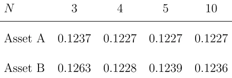
Table 6.2: Hodge’s Paradox – Approximation Formula

N 3 4 5 10

Asset A 0.1237 0.1227 0.1227 0.1227

Asset B 0.1263 0.1228 0.1239 0.1236

Explanation: Ranking measures for the distribution-only CARA version of the approximate ratio

(51)

6.2 Single Fund Asset Allocation and Ranking

Allocation

We use the generalized ratio to calculate the optimal asset allocation into the

S&P500, calculated based on monthly returns from January 1950 to June 2012,

versus a risk-free investment paying an annual interest rate rf = 5%. As noted

in Section (3.4.2), in the CRRA case we solve the “two fund separation” problem

simultaneously as part of the generating the ranking index. Table 6.3 reports the

associated values for the CRRA distribution-preference ranking measure.

Because the values shown in Table 6.3 are produced directly from the CRRA

ranking measure, we can “double check” the accuracy of our generalized ranking

calculation by also performing simulations on the orginal investor problem (2.1.1).

Recall that the generalized ranking measure is calculated based only on the

trans-lated moments of the underlying data. For the original investor problem, however,

we need to know the actual distribution in order to integrate the expectation

oper-ator. Since, we don’t have that information, we assume that the “true” distribution

is simply given by the histogram of our data and we then sample that data 100,000

times. Of course, this assumption could, in general, produce considerable error

be-cause it effectively eliminates the tails of the distribution, which could be especially

problematic with non-Normal risk. In the case of broad S&P500 index, however,

this effect appears to be small. Table 6.4 shows the results from simulation

(52)

(53)

Table 6.4: S&P500 – Simulation Results using the Investor Problem (2.1.1)

optimal allocation

CRRA(1) 143.03%

CRRA(2) 72.41%

CRRA(3) 48.45%

CRRA(4) 36.4%

CRRA(5) 29.15%

Explanation: CRRA(X) shows the distribution-preference CRRA ranking, where X is the

coef-ficient of risk aversion. CRRA results expressed as a percentage of wealth to be invested in the

fund.

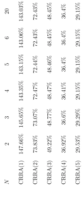
calculations produced by the Generalized Ratio with N = 20.

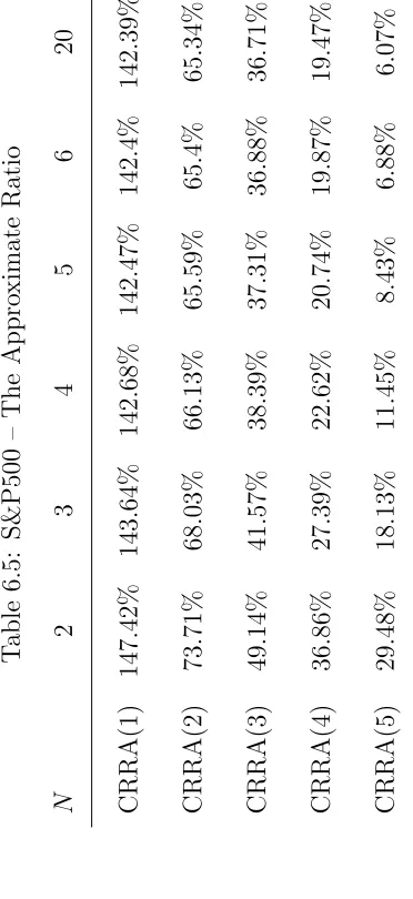
Table 6.5 also shows the results for the approximate risk measure. Notice that

the measure does fairly well at low values of risk aversion, but performs poorly at

higher values.

6.2.1 Fund-level Ranking

Sharpe ratios are routinely reported for publicly-traded mutual funds as well as

private funds. The purpose of these ratios is to provide investors with guidance

about how to rank funds. Mutual funds, hedge funds, and managers, therefore,

could easily produce the generalized ratio measure for the CRRA case for a range

(54)

(55)

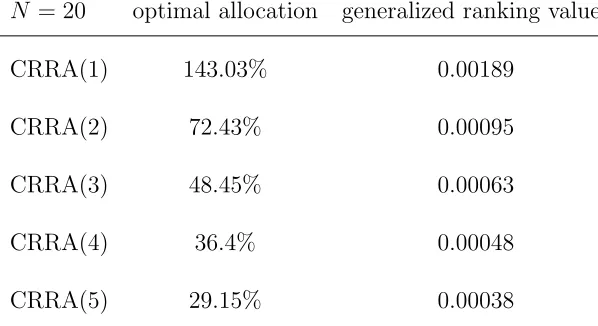
Table 6.6: Fund Ranking: The S&P500 Index as an Example Fund

N = 20 optimal allocation generalized ranking values

CRRA(1) 143.03% 0.00189

CRRA(2) 72.43% 0.00095

CRRA(3) 48.45% 0.00063

CRRA(4) 36.4% 0.00048

CRRA(5) 29.15% 0.00038

Explanation: Hypothetical rankings for CRRA(X), where X is the coefficient of risk aversion with

N = 20 adjusted cumulants.

sufficiently large value ofN.1 _{Table 6.6 shows the values that could be reported for}

a hypothetical S&P500 indexed fund.

6.3 Multi Asset Class Allocation

Borrowing the example of Goetzmann et al (2002), and subsequently followed by

Zakamouline and Koekebakker (2008), we now examine a portfolio with embedded

options. The underlying stock follows geometric Brownian motion with today’s

price normalized to $1. The price in 1 year is

S = exp

(µ−1

2σ

2_{) +}_σz

,

1_{As discussed in Section 3.4.2, the ranking measure is not monotone in the percent allocations}

invested into the fund (as shown in Table 6.4). Hence, the percent allocation is not a valid ranking

(56)

wherez is the standard Normal random variable. For simplicity, we use parameters

in Zakamouline and Koekebakker (2008): µ = 0.10, rf = 0.05, σ = 0.15. Also,

suppose there is a European put option with strike $0.88 and a European call

option with strike $1.12 that mature in 1 year. Using the Black-Scholes formula,

we calculated the non-arbitrage price for the put and call option today are $0.0079

and $0.0345 respectively. Denote (a1, a2) as the allocation in put and call options,

respectively. A positive value denotes buying the option while a negative value

means selling (a writer). To compute the optimal multi-asset allocation over the

puts and calls, we use a simple grid search with precision of 0.1 along the mesh,

thereby essentially ensuring us that our results are not being driven by potential

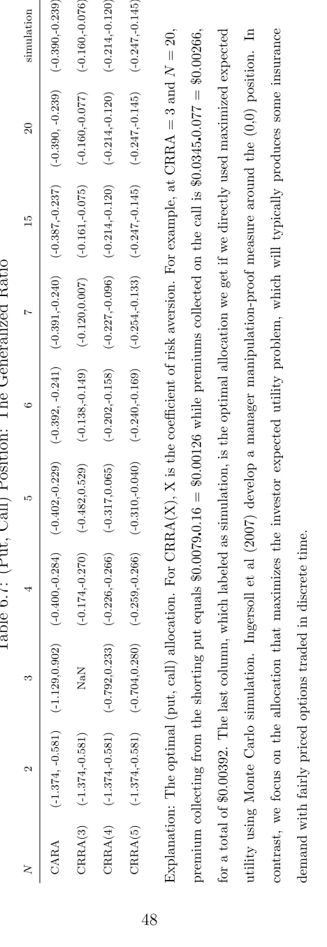
flaws in the global optimization routine.2

Our simulations find that a1 = −1.3739, a2 = −0.5807 maximizes the Sharpe

ratio. In other words, the Sharpe ratio suggests a strong amount of put writing

com-bined with a fair amount of call writing. In essence, the investor is short volatility,

collecting the insurance premium as the reward. Our generalized ratio, however,

suggests to short less put position and less call. In addition, we could match the

result where allocation is calculated from the original investor problem.

2_{Of course, with more assets, a grid search would quickly run into the “curse of dimensionality”}

(57)

(58)

Chapter 7 Conclusions

This paper derives a generalized ranking measure which, under a regularity

con-dition, is valid in the presence of a much broader assumption (utility, probability)

space than the Sharpe ratio and yet preserves wealth separation for the broad HARA

utility class. Our ranking measure can be used with “fat tails” as well as

multi-asset class portfolio optimization. We also explore the foundations of multi-asset ranking,

including proving a key impossibility theorem: any ranking measure that is valid at

non-Normal “higher moments” cannot generically be free from investor preferences.

Our simulation analysis demonstrates that the generalized ratio often produces very

different optimal portfolios relative to Sharpe, especially for multi-asset portfolios

where the assumption of Normality breaks down. The generalized ranking

mea-sure, therefore, can be used by investors and money managers, and could replace

(59)

Bibliography

[1] Agarwal, V. and Naik, N. Y. (2004). “Risk and Portfolio Decisions Involving

Hedge Funds, Review of Financial Studies , 17 (1), 63-98.

[2] Artzner, P., Delbaen, F., Eber, J.M. and Heath, D. (1999). “Coherent Measures

of Risk”. Mathematical Finance 9 (3): 203-228.

[3] Aumann, R. J., and Roberto S. (2008). “An economic index of riskiness.”

Journal of Political Economy, 116, 810-836.

[4] Barro, R. J. (2006). “Rare disasters and asset markets in the twentieth

cen-tury.” Quarterly Journal of Economics, 121, 823-866.

[5] Barro, R. J. (2009). “Rare disasters, asset prices, and welfare costs.” American

Economic Review, 99, 243-264.

[6] Bodie, Z., Merton, R.C. and Samuelson, W. (1991). “Labor supply exibility

and portfolio choice in a life cycle model.” Journal of Economic Dynamics and

(60)

[7] Brandt, M.W., Goyal, A., Santa-Clara, P. and Stroud. J.R. (2005). “A

sim-ulation approach to dynamic portfolio choice with an application to learning

about return predictability.” Review of Financial Studies, 18(3): 831.

[8] Brooks, C. and Kat, H. M., (2002). “The Statistical Properties of Hedge Fund

Index Returns and Their Implications for Investors”, Journal of Alternative

Investments, 5 (2), 26–44.

[9] Cherny, A. (2003). “Generalized Sharpe Ratios and Asset Pricing in Incomplete

Markets”, European Finance Review ,7 (2), 191-233

[10] Davila, E. (2010).“Myopic Portfolio Choice with Higher Cumulants”, Working

paper

[11] Dowd, K. (2000).“Adjusting for Risk: An Improved Sharpe Ratio”,

Interna-tional Review of Economics and Finance, 9, 209-222.

[12] Durrett, R. (2005). “Probability: Theory and Examples 3rd Edition”, Thomson

LearningT M

[13] Fama, E. (1965). “The Behaviour of Stock-Market Prices”, Journal of Business,

38, 34-105

[14] Foster, D. P., and Hart, S. (2009). “An operational measure of riskiness.”

(61)

[15] Gourio, F. (2012). “Disaster Risk and Business Cycles.” American Economic

Review, 102(6): 2734-66.

[16] Goetzmann, W., Ingersoll, J., Spiegel, M., and Welch, I. (2002). “Sharpening

Sharpe Ratios”, NBER Working Paper #9116.

[17] Hart, S. (2011). “Comparing risks by acceptance and rejection.” Journal of

Political Economy, 119, 617-638.

[18] Hodges, S. (1998). “A Generalization of the Sharpe Ratio and its Applications

to Valuation Bounds and Risk Measures”, Working Paper, Financial Options

Research Centre, University of Warwick.

[19] Ingersoll, J., Spiegel, M., and Goetzmann, W. (2007). “Portfolio Performance

Manipulation and Manipulation-proof Performance Measures”, Review of

Fi-nancial Studies, 20 (5), 1503-1546.

[20] Jensen, M.C. (1968). “The Performance of Mutual Funds in the Period

1945-1964,” Journal of Finance 23, 389-416.

[21] Jurczenko, E., and Maillet, B. (2006), “Theoretical Foundations of Asset

Al-locations and Pricing Models with Higher-order Moments”, JURCZENKO E.,

MAILLET B. (eds) , Multi-moment Asset Allocation and Pricing Models, John

A Sharper Ratio

University of Pennsylvania

ScholarlyCommons

A Sharper Ratio

Xingtan Zhang

A Sharper Ratio

A SHARPER RATIO

Xingtan Zhang

A DISSERTATION

in

Applied Mathematics and Computational Science

Presented to the Faculties of the University of Pennsylvania in Partial

Fulfillment of the Requirements for the Degree of Doctor of Philosophy

2013

Kent Smetters

Boettner Professor of Business Economics and Public Policy

Supervisor of Dissertation

Charles Epstein

Thomas A. Scott Professor of Mathematics

Graduate Group Chairperson

Robin Pemantle, Merriam Term Professor of Mathematics

Dedication

Acknowledgments

Contents

Chapter 1

Introduction

Chapter 2

The Investor Problem

2.1

Investor Problem

2.2

Ranking Definitions

2.3

The Sharpe Ratio

Chapter 3

Generalized Ratio Ranking

Measure

3.1

The Regularity Condition

3.2

HARA Utility

3.3

An Impossibility Theorem

3.4

Two Special Cases

3.4.1

CARA Utility

3.4.2

CRRA Utility

3.5

Extension to Multiple Asset Classes

Chapter 4

Foundations of Ranking

4.1

Adjusted Cumulants

4.1.1

Definitions

4.1.2

Calculating Adjusted Cumulants

4.2

Ranking Measure with Short Trading Times

4.3

Understanding the Sharpe Ratio

4.4

Generalization of the Skewness Preference

Chapter 5

An Approximation Formula

Chapter 6

Applications

6.1

Hodge’s (1998) Paradox

6.2

Single Fund Asset Allocation and Ranking

6.2.1

Fund-level Ranking

6.3

Multi Asset Class Allocation

Chapter 7

Conclusions

Bibliography