University of Pennsylvania
ScholarlyCommons
Publicly Accessible Penn Dissertations
1-1-2015
Fast Linear Algorithms for Machine Learning
Yichao Lu
University of Pennsylvania, [email protected]
Follow this and additional works at:http://repository.upenn.edu/edissertations
Part of theComputer Sciences Commons, and theStatistics and Probability Commons
This paper is posted at ScholarlyCommons.http://repository.upenn.edu/edissertations/1091
For more information, please [email protected]. Recommended Citation
Lu, Yichao, "Fast Linear Algorithms for Machine Learning" (2015).Publicly Accessible Penn Dissertations. 1091.
Fast Linear Algorithms for Machine Learning
Abstract
Nowadays linear methods like Regression, Principal Component Analysis and Canoni- cal Correlation Analysis are well understood and widely used by the machine learning community for predictive modeling and feature generation. Generally speaking, all these methods aim at capturing interesting subspaces in the original high dimensional feature space. Due to the simple linear structures, these methods all have a closed form solution which makes computation and theoretical analysis very easy for small datasets. However, in modern machine learning problems it's very common for a dataset to have millions or billions of features and samples. In these cases, pursuing the closed form solution for these linear methods can be extremely slow since it requires multiplying two huge matrices and computing inverse, inverse square root, QR
decomposition or Singular Value Decomposition (SVD) of huge matrices. In this thesis, we consider three fast al- gorithms for computing Regression and Canonical Correlation Analysis approximate for huge datasets.
Degree Type
Dissertation
Degree Name
Doctor of Philosophy (PhD)
Graduate Group
Applied Mathematics
First Advisor
Dean P. Foster
Keywords
canonical correlation analysis, gradient methods, large scale, linear regression, machine learning
Subject Categories
FAST LINEAR ALGORITHMS FOR MACHINE LEARNING
Yichao Lu
A DISSERTATION
in
Applied Mathematics and Computational Science
Presented to the Faculties of the University of Pennsylvania in Partial
Ful-fillment of the Requirements for the Degree of Doctor of Philosophy
2015
Supervisor of Dissertation
Dean P. Foster, Professor of Statistics
Graduate Group Chairperson
Charles L. Epstein, Thomas A. Scott Professor of Mathematics
Dissertation Committee:
Dean P. Foster, Professor of Statistics
Acknowledgments
First and Foremost, I would like to express my sincere gratitude to my Advisor Dean
Foster for his support during my PhD study. His broad knowledge, sharp intuition, patient
guidance and passion about problems in statistics and machine learning providing me
with an excellent atmosphere for doing research.
I am deeply grateful to Professor Lyle Ungar, Zonging Ma and Robert Stine for many
stimulating ideas and valuable discussions at the StatNLP reading group and when I’m
preparing for my thesis. I would like to thank Professor Charles Epstein for providing
me the wonderful opportunity to study in the AMCS program and his kind support at the
beginning of my PhD career.
I would like to thank my fellow PhD students Paramveer Dhillon, Jordan Rodu,
Pe-ichao Peng, Zhuang Ma, Joao Sedoc, Wei Han, Fan Yang, Anru Zhang, Fan Zhao, Pengfei
Zheng, Shi Gu, Muzhi Yang, Yuanpei Cao and Ke Zeng. It’s a great honor for me to spend
my Phd years studying and having fun with a group of smart and interesting friends.
Last but not the least, I want to thank my family for their support, encouragement,
ABSTRACT
FAST LINEAR ALGORITHMS FOR MACHINE LEARNING
Yichao Lu
Dean P. Foster, Advisor
Nowadays linear methods like Regression, Principal Component Analysis and
Canoni-cal Correlation Analysis are well understood and widely used by the machine learning
community for predictive modeling and feature generation. Generally speaking, all these
methods aim at capturing interesting subspaces in the original high dimensional feature
space. Due to the simple linear structures, these methods all have a closed form
so-lution which makes computation and theoretical analysis very easy for small datasets.
However, in modern machine learning problems it’s very common for a dataset to have
millions or billions of features and samples. In these cases, pursuing the closed form
solution for these linear methods can be extremely slow since it requires multiplying two
huge matrices and computing inverse, inverse square root, QR decomposition or Singular
Value Decomposition (SVD) of huge matrices. In this thesis, we consider three fast
al-gorithms for computing Regression and Canonical Correlation Analysis approximate for
huge datasets.
For linear regression, we consider a combination of two well known algorithms,
matri-ces in our problems are huge, we use the fast randomized SVD algorithm proposed by
Halko et al. for computing the top principal components. We show that a this
com-bination will provide an approximate regression solution which is both fast and robust.
Theoretical analysis and empirical results about the convergence speed and statistical
ac-curacy of our algorithm are provided in Chapter 2.
For Canonical Correlation Analysis (CCA), we consider two different approaches.
In the first approach, we reduce the CCA problem to a sequence of iterative regression
problems. Plug in the fast regression algorithm into this framework generates our first
fast CCA algorithm. A detailed analysis about the convergence speed and empirical
per-formance of this algorithm is provide in Chapter 3. In the second approach, we regard
CCA as a constrained optimization problem and solve it by a gradient style algorithm.
The benefit of the second approach over the first approach is in the second approach, the
gradient style updates allows the CCA subspace estimator to improve after every
itera-tion while in the first approach the CCA subspace estimator can only be improved when
a reasonably accurate regression is performed. Based on this observation a stochastic
version of the second CCA approach is proposed which is very fast if aim at moderate
Contents
1 Introduction 1
2 Fast Ridge Regression Algorithm 6
2.1 Introduction . . . 6
2.2 The Algorithm . . . 8
2.2.1 Description of the Algorithm . . . 8
2.2.2 Computational Cost . . . 13
2.3 Theorems . . . 15
2.3.1 The Fixed Design Model . . . 16
2.4 Experiments . . . 19
2.4.1 Simulated Data . . . 20
2.4.2 Real Data . . . 25
2.5 summary . . . 29
3.2 Background: Canonical Correlation Analysis . . . 33
3.2.1 Definition . . . 33
3.2.2 CCA and SVD . . . 33
3.3 Compute CCA by Iterative Least Squares . . . 34
3.3.1 A Special Case . . . 36
3.3.2 General Case . . . 36
3.4 Algorithm . . . 37
3.4.1 LING: a Gradient Based Least Square Algorithm . . . 37
3.4.2 Fast Algorithm for CCA . . . 40
3.4.3 Error Analysis of L-CCA . . . 41
3.5 Experiments . . . 42
3.5.1 Penn Tree Bank Word Co-ocurrence . . . 46
3.5.2 URL Features . . . 48
3.6 Conclusion and Future Work . . . 50
4 Augmented Approximate Gradient Algorithm for Large Scale Canonical Cor-relation Analysis 51 4.1 Introduction . . . 51
4.1.1 Background . . . 51
4.1.2 Related Work . . . 54
4.1.3 Main Contribution . . . 55
4.2.1 An Optimization Perspective . . . 56
4.2.2 AppGradScheme . . . 60
4.2.3 General Rank-kCase . . . 64
4.2.4 Kernelization . . . 66
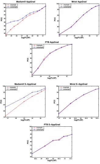
4.3 StochasticAppGrad . . . 67
4.4 Experiments . . . 69
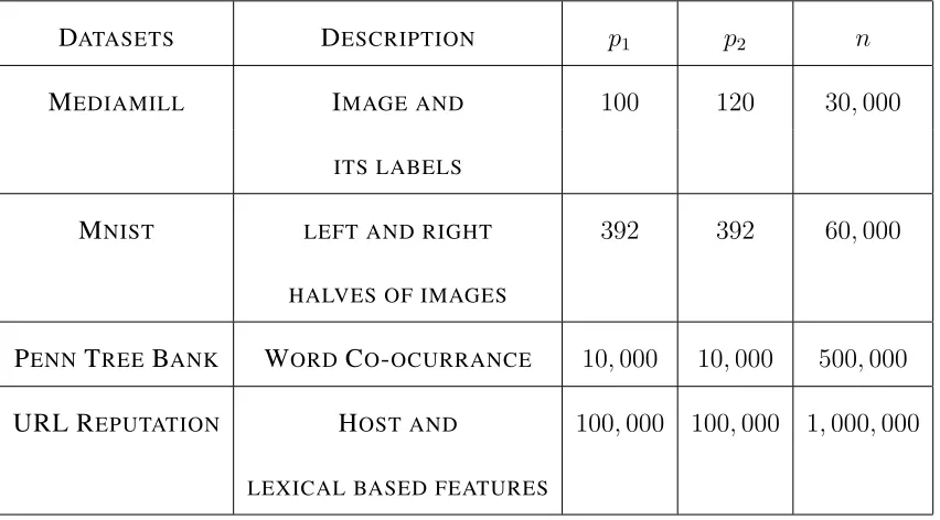
4.4.1 Details of Datasets . . . 70
4.4.2 Implementations . . . 71
4.4.3 Summary of Results . . . 73
4.5 Conclusions and Future Work . . . 76
Appendices 78 A Appendix for Chapter 3 79 A.1 Proof of Theorem 3.3.1 . . . 79
A.2 Randomized Algorithm for Finding Top Singular Vectors . . . 80
A.3 Gradient Descent with Optimal Step Size . . . 81
A.4 Error Analysis of LING . . . 83
A.4.1 Proof of Theorem 3.4.2 . . . 86
Chapter 1
Introduction
Linear methods like Regression, Principal Component Analysis and Canonical
Correla-tion Analysis are well understood and widely used by the machine learning community
for predictive modeling and feature generation. Generally speaking, all these methods
aim at capturing interesting subspaces in the original high dimensional feature space.
Due to the simple linear structures, these methods all have a closed form solution. For
small datasets, one can implement these methods in R, Matlab, Python or other platforms
as long as the computational tools can perform some basic linear algebra operations like
matrix multiplication, matrix inversion, singular value decomposition, QR
decomposi-tion. However, in modern machine learning problems it’s very common for a dataset
to have millions or billions of features and samples. For example, in Natural Language
Processing (NLP), using only unigram model will generate a feature space the dimension
moderate size and can get much larger for huge corpora. Moreover, it’s very common
to use bigram (or trigram) model for NLP tasks which make the feature dimension
vo-cabulary size squared (or cubed). Another example is in collaborative filtering where
the algorithms often need to handle an input matrix with size number of products times
number of customers which can easily reach millions. In these cases, pursuing the closed
form solution for these linear methods can be extremely slow since it requires
multiply-ing two huge matrices and computmultiply-ing inverse, inverse square root, QR decomposition or
Singular Value Decomposition (SVD) of huge matrices. In this thesis, we consider three
fast algorithms for computing these linear methods approximately on huge datasets.
Fast Principal Component Analysis algorithms has been well studied in the past few
years. One well known approach is the randomized SVD algorithm proposed by [28, 30]
which is extremely fast if one is only interested in computing the top few principal
com-ponents (singular vectors). In the randomized SVD algorithm, first a random projection
is performed to generate an estimator of the subspace spanned by the top few left
sin-gular vectors. Then this subspace is used to project the original huge data matrix down
to a much smaller size and it suffices to compute the SVD of the small matrix. Detailed
theoretical analysis of this algorithm is available in [28] and a brief introduction of the
algorithm will be provided in chapter 2 and appendix since we are going to use it as a
Fast Regression (or Least Squares) has also been well studied and a lot of algorithms
have been proposed based on the idea of random projection or subsampling. When the
number of observations is much larger than the number of features, [21, 6, 47] use
dif-ferent kinds of fast random projections that approximately preserve inner products in the
Euclidian space to reduce the actual sample size of the problem and then solve the least
squares problem on reduced dataset. Random projection with such properties are
some-times called fast Johnson-Lindenstrauss transforms. Different random projections with
this property are introduced in [2, 48, 54] with concentration bounds on how well the
inner product is preserved. These techniques are applied in a fast ridge regression
algo-rithm by [39] when the number of features are much larger than the number of samples.
Another slightly different idea is to subsample the observations from some non-uniform
distribution determined by the statistical leverage as discussed in [20, 44]. The statistical
accuracy of the above algorithms are discussed by [42, 16] in which they also proposed
some improvements based on the statistical analysis.
However, the main draw back for the fast regression algorithms is that they are still
very slow for problems with a huge amount of features. In fact, the acceleration of these
algorithms comes from a fast approximation of the matrix multiplication X>X where
X ∈ n×pis a data matrix withn samples andpfeatures. On the other hand, these
al-gorithms still need to invert ap×psquare matrix which is very slow whenpis large. To
components by the randomized SVD algorithm and then regress only on the top
princi-pal components (i.e. run a principrinci-pal component regression or PCR) or regard regression
as a quadratic minimization problem and approximate the solution by gradient descent
(GD). Both algorithms are trading accuracy for speed. For PCR, if only a few principal
component are selected, then the algorithm will be extremely fast but will probably miss
interesting signals on the bottom principal components. If a relatively large amount of
principal components are selected (but not overfit), more signals will be captured but the
algorithm will slow down. For GD, every gradient iteration is super fast and as the
num-ber of iterations increases, the solution gets more accurate but the algorithm takes more
time. In our fast algorithm [58], we combine PCR and GD together to get a new fast
regression algorithm which archives a better tradeoff between accuracy and speed. As
shown in the experiments, to achieve a certain accuracy, the number of principal
compo-nents and gradient iterations in our algorithm is significantly less than running PCR or
GD alone.
Fast Canonical Correlation Analysis (CCA) algorithm is a relatively new topic.
Fol-lowing the same idea in regression, [5] applied fast Johnson-Lindenstrauss transform to
reduce the sample size of the data matrices and then compute CCA on the reduced data.
Same as regression, this algorithm only works for dataset with a large sample size but
not with a large amount of features. In this thesis we propose two fast CCA algorithms
CCA subspace given to huge data matrices. Our algorithms can handle the case where
the number of features is extremely large and works well with sparse data matrices. In
the first approach [40], we reduce the CCA algorithm to several regression problems and
apply fast regression algorithms to obtain a fast CCA algorithm. In the second approach,
we view CCA as a constrained optimization problem and propose a gradient style
itera-tive algorithm which will converge to the true CCA subspace. It’s non trivial since the
optimization problem for CCA is not convex. Moreover, our second algorithm can also
be interpreted as a improvement of our first algorithm since it’s essentially replacing a
fast regression in the first algorithm with a simple gradient step. It’s easy to generalize
our second algorithm to an online (stochastic) setting due to its gradient nature. In fact,
as shown by the experiments, a stochastic version of the second algorithm can be even
faster than the batch version if we aim at moderate accuracy.
The thesis is organized as follows: in Chapter 2, we introduce the fast regression
algorithm which is a combination of two classical algorithms PCR and GD. In Chapter
3, we discuss the regression formulation of CCA and apply the fast regression algorithm
from Chapter 2 to get our first fast CCA algorithm. In Chapter 4, we introduce both the
batch and stochastic version of our second fast CCA algorithm. The thesis is organized in
a way that chapter 2,3,4 can be read separately as three independent papers. Each chapter
will include some simple theorem proofs, but the long and complicated proofs will be
Chapter 2
Fast Ridge Regression Algorithm
2.1
Introduction
Ridge Regression (RR) is one of the most widely applied penalized regression algorithms
in machine learning problems. SupposeXis then×pdesign matrix andYis then×1
response vector, ridge regression tries to solve the problem
ˆ
β = arg min
β∈RpkXβ−Yk
2
+nλkβk2 (2.1.1)
which has an explicit solution
ˆ
β = (X>X+nλ)−1X>Y (2.1.2)
However, for modern problems with huge design matrix X, computing (2.1.2) costs
O(np2)FLOPS. Whenp > n1one can consider the dual formulation of (2.1.1) which
summary, trying to solve (2.1.1) exactly costs O(npmin{n, p}) FLOPS which can be
very slow.
There are faster ways to approximate (2.1.2) when computational cost is the concern.
One can view RR as an optimization problem and use Gradient Descent (GD) which
takesO(np)FLOPS in every iteration. However, the convergence speed for GD depends
on the spectrum ofXand the magnitude ofλ. WhenXis ill conditioned andλis small,
GD requires a huge number of iterations to converge which makes it very slow. For huge
datasets, one can also apply stochastic gradient descent (SGD) [59, 34, 11], a powerful
tool for solving large scale optimization problems.
Another alternative for regression on huge datasets is Principal Component Regression
(PCR) as mentioned in [4, 35], which runs regression only on the topk1principal
compo-nents (PCs) of theXmatrix. PCA for hugeXcan be computed efficiently by randomized
algorithms like [29, 30]. The cost for computing top k1 PCs of X isO(npk1)FLOPS.
The connection between RR and PCR is well studied by [18]. The problem of PCR is that
when a large proportion of signal sits on the bottom PCs, it has to regress on a lot of PCs
which makes it both slow and inaccurate (see later sections for detailed explanations).
In this paper, we propose a two stage algorithm LING1which is a faster way of
comput-ing the RR solution (2.1.2). A detailed description of the algorithm is given in section
2.2. In section 2.3, we prove that LING has the same risk as RR under the fixed design
setting. In section 2.4, we compare the performance of PCR, GD, SGD and LING in
terms of prediction accuracy and computational efficiency on both simulated and real
data sets.
2.2
The Algorithm
2.2.1
Description of the Algorithm
LING is a two stage algorithm. The intuition of LING is quite straight forward. We start
with the observation that regressingYonX(OLS) is equivalent to projectingYonto the
span ofX. LetU1 denote the topk2 PCs (left singular vectors) ofXand letU2 denote
the remaining PCs. The projection ofYonto the span ofXcan be decomposed into two
orthogonal parts, the projection ontoU1 and the projection ontoU2. In the first stage, we
pick a k2 pand the projection ontoU1 can be computed directly byYˆ1 = U1U>1Y
which is exactly the same as running a PCR on top k2 PCs. For huge X, computing
the top k2 PCs exactly is very slow, so we use a faster randomized SVD algorithm for
computingU1 which is proposed by [28] and described below. In the second stage, we
first compute Yr = Y −Yˆ1 and Xr = X −U1U>1X which are the residuals of Y
and X after projecting onto U1. Then we compute the projection of Y onto the span
ofU2 by solving the optimization problemminˆγ2∈RpkXrγˆ2−Yrk
2+nλkγˆ
2kwith GD
(Algorithm 3). Finally, since RR shrinks the projection ofYontoX(the OLS solution)
via regularization, we also shrink the projections in both stages accordingly. Shrinkage in
Algorithm 1LING
Input : Data matrix X,Y. U1, an orthonormal matrix consists of topk2 PCs of X.
d1, d2, ...dk2, topk2 singular values ofX. Regularization parameterλ, an initial vector
ˆ
γ2,0 and number of iterationsn2for GD .
Output : γˆ1,s,ˆγ2, the regression coefficients.
1.RegressYonU1, letγˆ1 =U>1Y.
2.Compute the residual of previous regression problem. LetYr =Y−U1γˆ1.
3.Compute the residual ofXregressing onU1. UseXr =X−U1U>1Xto denote the
residual ofX.
4.Use gradient descent with optimal step size with initial valueγˆ2,0 (see algorithm 3)
to solve the RR problemminγˆ2∈RpkXrˆγ2−Yrk
2+nλkγˆ 2k2.
5. Compute a shrinkage version ofˆγ1by(ˆγ1,s)i = d2
i d2
i+nλ (ˆγ1)i
6.The final estimator isYˆ =U1γˆ1,s+Xrγˆ2.
in the second stage is performed by adding a regularization term to the optimization
problem mentioned above. Detailed description of LING is shown in Algorithm 1.
Remark 2.2.1. LING can be regarded as a combination of PCR and GD. The first stage
of LING is a crude estimation of the projection ofY ontoX and the second stage adds
a correction to the first stage estimator. Since we do not need a very accurate estimator
in the first stage it suffices to pick a very small k2 in contrast with thek1 PCs needed
for PCR. In the second stage, the design matrixXr is a much better conditioned matrix
Algorithm 2Random SVD
Input : design matrixX, target dimensionk2, number of power iterationsi.
Output : U1 ∈ n×k2, the matrix of topk2 left singular vectors ofX, d1, d2, ...dk2,
the topk2 singular values ofX.
1.Generate random matrixR1 ∈p×k2with i.i.d standard Gaussian entries.
2.Estimate the span of topk2left singular vectors ofXbyA1 = (XX>)iXR1.
3.Use QR decomposition to computeQ1which is an orthonormal basis of the column
space ofA1.
4.Compute SVD of the reduced matrixQ>1X=U0D0V>0.
5.U1 =Q1U0gives the topk2 singular vectors ofXand the diagonal elements ofD0
gives the singular values.
introduced in section 2.2, Algorithm 3 converges much faster with a better conditioned
matrix. Hence GD in the second stage of LING converges faster than directly applying
GD for solving (2.1.1). The above property guarantees that LING is both fast and
accu-rate compared with PCR and GD. More details about on the computational cost will be
discussed in section 2.2.2.
Remark2.2.2. Algorithm 2 is essentially approximating the subspace of top left singular
vectors by random projection. It provides a fast approximation of the top singular
val-ues and vectors for large X when computing the exact SVD is very slow. Theoretical
guarantees and more detailed explanations can be found in [28]. Empirically we find in
Algorithm 3Gradient Descent with Optimal Step Size (GD)
Goal : Solve the ridge problemminˆγ∈RpkXˆγ−Yk2+nλkˆγk2.
Input : Data matrix X, Y, regularization parameter λ, number of iterations n2, an
initial vectorˆγ0
Output : γˆ
fort = 0ton2−1do
Q= 2X>X+ 2nλI
wt = 2X>Y−Qˆγt
st=
w>
t wt w>
t Qwt
. stis the step size which makes the target function decrease the most in
directionwt.
ˆ
γt+1 = ˆγt+st·wt.
randomness which makes PCR perform badly. On the other hand, LING is much more
robust since in the second stage it compensates for the signal that was missed in the first
stage. In all the experiments, we seti= 1.
The shrinkage step (step 5) in Algorithm 1 is only necessary for theoretical purposes
since the goal is to approximate Ridge Regression which shrinks the Least Squares
es-timator over all directions. In practice shrinkage over the top k2 PCs is not necessary.
Usually the number of PCs selected (k2) is very small. From the bias variance trade off
perspective, the variance reduction gained from the shrinkage over topk2 PCs is at most
O(k2
n)under the fixed design setting [18] which is a tiny number. Moreover, since the
top singular values ofX>Xare usually very large compared withnλin most real
prob-lems, the shrinkage factor d2i d2
i+nλ will be pretty close to
1for top singular values. We use
shrinkage in Algorithm 1 because the risk of the shrinkage version of LING is exactly
the same as RR as proved in section 2.3.
Algorithm 2 can be further simplified if we skip the shrinkage step mentioned in previous
paragraph. Instead of computing the top k2 PCs, the only thing we need to know is the
subspace spanned by these PCs since the first stage is essentially projectingY onto this
subspace. In other words, we can replace U1 in step 1, 2, 3 of Algorithm 1 with Q1
obtained in step 3 of Algorithm 2 and directly letYˆ =Q1ˆγ1+Xrγˆ2. In the experiments
2.2.2
Computational Cost
We claim that the cost of LING isO np(k2+n2)
wherek2 is the number of PCs used
in the first stage andn2 is the number of iterations of GD in the second stage. According
to [28], the dominating step in Algorithm 2 is computing(XX>)iXR
1andQ>1Xwhich
costs O(npk2)FLOPS. Computing γˆ1 andYr costs less than O(npk2). ComputingXr
costs O(npk2). So the computational cost before the GD step is O(npk2). For the GD
stage, note that in every iterationQnever needs to be constructed explicitly. While
com-puting wt and st, always multiplying matrix and vector first gives a cost of O(np)for
every iteration. So the cost for GD stage isO(n2np). Add all pieces together the cost of
LING isO np(k2+n2)
FLOPS.
Let n1 be the number of iterations required for solving (2.1.1) directly by GD and k1
be the number of PCs used for PCR. It’s easy to check that the cost for GD is O(n1np)
FLOPS and the cost for PCR is O(npk1). As mentioned in remark 2.2.1, the advantage
of LING over GD and PCR is thatk1andn1might have to be really large to achieve high
accuracy but much smaller values of the pair(k2,n2)will work for LING.
In the remaining part of the chapter we use ”signal on certain PCs” to refer to the
projec-tion ofY onto certain principal components ofX. Consider the case when the signal is
widely spread among all PCs (i.e. the projection ofY onto the bottom PCs of Xis not
very small) instead of concentrating on the top ones, k1 needs to be large to make PCR
perform well since the signal on bottom PCs are discarded by PCR. But LING does not
estimated in the second GD stage. Therefore LING is able to recover most of the signal
even with a smallk2.
In order to understand the connection between accuracy and number of iterations in
Al-gorithm 3 , we state the following theorem in [1]:
Theorem 2.2.3. Letg(z) = 12z>M z+q>z be a quadratic function whereM is a PSD
matrix. Supposeg(z)achieves minimum atz∗. Apply Algorithm 3 to solve the
minimiza-tion problem. Let zt be the z value after t iterations, then the gap between g(zt) and
g(z∗), the minimum of the objective function satisfies
g(zt+1)−g(z∗)
g(zt)−g(z∗) ≤C =
A−a
A+a
2
(2.2.1)
whereA, aare the largest and smallest eigenvalue of theM matrix.
Theorem 2.2.3 shows that the sub optimality of the target function decays
exponen-tially as the number of iterations increases and the speed of decay depends on the largest
and smallest singular value of the PSD matrix that defines the quadratic objective
func-tion. If we directly apply GD to solve (2.1.1), Let f1(β) = kXβ − Yk2 +nλkβk2.
Assumef1 reaches its minimum atβˆ. Letβtˆ be the coefficient aftertiterations and letdi
denote theithsingular value ofX. Applying theorem 2.2.3, we have f1( ˆβt+1)−f1( ˆβ)
f1( ˆβt)−f1( ˆβ)
≤C =
d2
1−d2p d2
1+d2p+ 2nλ
2
(2.2.2)
Similarly for the second stage of LING, Letf2(γ2) = kXrγ2−Yrk2+nλkγ2k2. Assume
f2 reaches its minimal atγˆ2. We have
f2(ˆγ2,t+1)−f2(ˆγ2)
f2(ˆγ2,t)−f2(ˆγ2)
≤C=
d2
k2+1
d2
k2+1+ 2nλ
2
In most real problems, the top few singular values ofX>Xare much larger than the other
singular values and nλ. Therefore the constantC obtained in (2.2.2) can be very close
to 1 which implies that the GD algorithm converges very slowly. On the other hand,
removing the top few PCs will make C in (2.2.3) significantly smaller than 1. In other
words, GD may take a lot of iterations to converge when solving (2.1.1) directly while
the second stage of LING takes much less iterations to converge. This can also be seen
in the experiments of section 2.4.
2.3
Theorems
In this section we compute the risk of LING estimator (explained below) under the fixed
design setting. For simplicity, assumeU1,D0 generated by Algorithm 2 give exactly the
topk2left singular vectors and singular values ofXand GD in step 4 of Algorithm 1
con-verges to the optimal solution. LetX=UDV>be the SVD ofXwhereU= (U1,U2)
and V = (V1,V2). Here U1,V1 are top k2 singular vectors and U2,V2 are bottom
p−k2 singular vectors. Let D = diag(D1,D2) where D1 ∈ k2 ×k2 contains topk2
singular values denoted by d1 ≥ d2 ≥ ... ≥ dk2 and D2 ∈ p−k2 ×p−k2 contains
bottomp−k2singular values. LetD3 =diag(0,D2)(replaceD1 inDby a zero matrix
2.3.1
The Fixed Design Model
AssumeX,Ycomes from the fixed design modelY =Xβ+where∈n×1are i.i.d
noise with mean0and varianceσ2. HereXis fixed and the randomness ofYonly comes
from. Note thatX=U1D1V>1 +Xr, the fixed design model can also be written as
Y = (U1D1V>1 +Xr)β+=U1γ1+Xrγ2+
where γ1 = D1V1>β and γ2 = β. We use the l2 distance between E(Y|X) (the best
possible prediction given X under l2 loss) and Yˆ = U1γˆ1,s +Xrγˆ2 (the prediction by
LING) as the loss function, which is called risk in the following discussions. Actually
E(Y|X) = Xβis linear inXunder fixed design model. The risk of LING can be written
as
1
nEkE(Y|X)−U1γˆ1,s−Xrˆγ2k
2
= 1
nEkU1γ1+Xrγ2−U1γˆ1,s−Xrγˆ2k
2
We can further decompose the risk into two terms:
1
nEkU1γ1+Xrγ2−U1γˆ1,s −Xrˆγ2k
2
=
1
nEkU1γ1−U1γˆ1,sk
2+ 1
nEkXrγ2−Xrˆγ2k
2
(2.3.1)
becauseU>1Xr = 0. Note that here the expectation is taken with respect to.
Let’s calculate the two terms in (2.3.1) separately. For the first term we have:
Lemma 2.3.1.
1
nEkU1γ1 −U1γˆ1,sk
2
= 1
n k2
X
j=1
d4
jσ2+γ12,jn2λ2 (d2
j +nλ)2
(2.3.2)
Proof. LetS ∈ k2 ×k2 be the diagonal matrix withSj,j =
d2j d2
j+nλ. So we haveγˆ1,s = SU>1Y =Sγ1+SU1>,E(ˆγ1,s) =Sγ1.
1
nEkU1γ1−U1ˆγ1,sk
2
= 1
nEkU1E(ˆγ1,s)−U1ˆγ1,sk
2
+1
nkU1γ1−U1E(ˆγ1,s)k
2
= 1
nEkU1SU
>
1k 2+ 1
nkγ1−Sγ1k
2
= 1
nETr(U1S
2U>
1
>
) + 1
nkγ1−Sγ1k
2
= 1
nETr(S
2)σ2+ 1
nkγ1−Sγ1k
2 = 1 n k2 X j=1 d4
jσ2+γ12,jn2λ2 (d2
j +nλ)2
Now consider the second term in (2.3.1).
Note that
Xr=UD3V>
The residualYr after the first stage can be represented by
Yr =Y−U1γˆ1 = (I −U1U1>)Y =Xrγ2+ (I−U1U>1)
and the optimal coefficient obtained in the second GD stage is
ˆ
γ2 = (X>rXr+nλI)−1X>rYr
Lemma 2.3.2.
EkXrγ2−Xrˆγ2k2 =
p
X
i=k2+1
1 (d2
i +nλ)2
(d4iσ2+nλ2d2iα2i) (2.3.3)
whereαi is theithelement ofα =V>γ2
Proof. First define
Xλ = X>rXr+nλI
Dλ = D23+nλI
EkXrγ2 −Xrˆγ2k2 = kXrγ2 −XrE(ˆγ2)k2 (2.3.4)
+ EkXrE(ˆγ2)−Xrγˆ2k2 (2.3.5)
Consider (2.3.4) and (2.3.5) separately.
(2.3.4) = kXrX−λ1X
>
rXrγ2−Xrγ2k2
= kUD3D−λ1D23V
>
γ2−UD3V>γ2k2
= kD3D−λ1D
2
3α−D3αk2
= p
X
i=k2+1
α2id2i( nλ d2
i +nλ
)2
(2.3.5) =E2kXrX
−1
λ X
> r2k2
= E2Tr XrX
−1
λ X
>
rXrX−λ1X > r2>2
= E2Tr D3D
−1
λ D
2 3D
−1
λ D3U
> 2>2U
= Tr D3D−λ1D23D
−1
λ D3E2[U
>
Note that
E2[U
>
2>2U] =diag(0, Ip−k2)σ
2
(diag(0, Ip−k2)replace the topk2×k2 block of the identity matrix with 0),
(2.3.5) = p
X
i=k2+1
d4
i (d2
i +nλ)2
σ2 (2.3.6)
Add the two terms together finishes the proof.
Plug (2.3.2) (2.3.3) into (2.3.1) we have
Theorem 2.3.3. The risk of LING algorithm under fixed design setting is
1 n
k2
X
j=1
d4
jσ2+γ12,jn2λ2 (d2
j +nλ)2
+ 1
n p
X
i=k2+1
d4iσ2+n2λ2d2iα2i (d2
i +nλ)2
(2.3.7)
Remark2.3.4. This risk is the same as the risk of ridge regression provided by Lemma 1
in [18]. Actually, LING gets exactly the same prediction as RR on the training dataset.
This is very intuitive since on the training set LING is essentially decomposing the RR
solution into the first stage shrinkage PCR predictor on topk2 PCs and the second stage
GD predictor over the residual spaces as explained in section 2.2.
2.4
Experiments
In this section we compare the accuracy and computational cost (evaluated in terms of
FLOPS) of 3 different algorithms for solving Ridge Regression: Gradient Descent with
Here SVRG is an improved version of stochastic gradient descent which achieves
ex-ponential convergence with constant step size. We also consider Principal Component
Regression (PCR) [4, 35] which is another common way for running large scale
regres-sion. Experiments are performed on 3 simulated models and 2 real datasets. In general,
LING performs well on all 3 simulated datasets while GD, SVRG and PCR fails in some
cases. For two real datasets, all algorithms give reasonable performance while SVRG
and LING are the best. Moreover, both stages of LING require only a moderate amount
of matrix multiplications each costO(np), much faster to run on matlab compared with
SVRG which contains a lot of loops.
2.4.1
Simulated Data
Three different datasets are constructed based on the fixed design model Y = Xβ +
whereXis of size2000×1500. In the three experimentsXandβare generated randomly
in different ways (more details in following sections) and i.i.d Gaussian noise is added
to Xβ to get Y. Then GD, SVRG, PCR and LING are performed on the dataset. For
GD, we try different number of iterationsn1. For SVRG, we vary the number of passes
through data denoted bynSVRG. The numbers of iterations SVRG takes equals the number
of passes through data times sample size and each iteration takesO(p)FLOPS. The step
size of SVRG is chosen by cross validation but this cost is not considered when evaluating
the total computational cost. Note that one advantage of GD and LING is that due to the
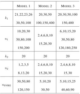
Table 2.1: parameter setup for simulated data
MODEL1 MODEL2 MODEL3
k1
21,22,23,26
30,50,100
20,30,50
100,150,400
20,30,50,100
150,400
n1
10,20,30
50,80,100
150,200
2,4,6,8,10
15,20,30
6,10,15,20
30,50,80
120,180,250
k2 20 20 20
n2
1,2,3,5
8,13,20
2,4,6,8,10
15,20,30
2,4,6,8,10
15,30
nSVRG
30,50,80
120,150
5,10,20
30,50
5,10,15,25
40,60,90
from the data without cross validation which introduces extra cost. For PCR we pick
different number of PCs (k1). For LING we pick top k2 PCs in the first stage and try
different number of iterationsn2in the second stage. The computational cost and the risk
of the four algorithms are computed. The above procedure is repeated over 20 random
generations ofX,βandY. The risk and computational cost of the traditional RR solution
(2.1.2) for every dataset is also computed as a benchmark.
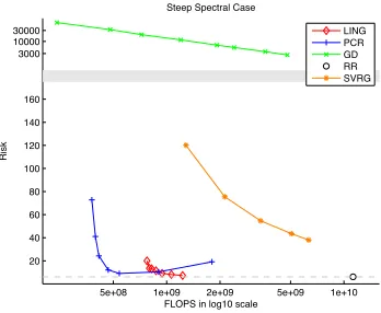
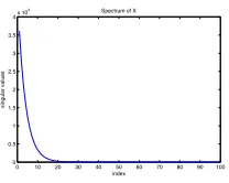
Model 1
In this model the design matrixXhas a steep spectrum. The top 30 singular values ofX
decay exponentially as 1.3i wherei = 40,39,38...,11. The spectrum ofXis shown in
figure 2.4. To generateX, we fix the diagonal matrixDewith the designed spectrum and
constructXbyX=UeDeVe>whereUe,Veare two random orthonormal matrices. The
elements ofβare sampled uniformly from interval[−2.5,2.5]. Under this set up, most of
the energy of the Xmatrix lies in top PCs since the top singular values are much larger
than the remaining ones so PCR works well. But as indicated by (2.2.2), the convergence
of GD is very slow.
The computational cost and average risk of the four algorithms and also the RR solution
(2.1.2) over 20 repeats are shown in figure 2.1. As shown in figure 2.1 both PCR and
LING work well by achieving risk close to RR at less computational cost. SVRG is
worse than PCR and LING but much better than GD.
Model 2
In this model the design matrix X has a flat spectrum. The singular values of X are
sampled uniformly from[ √
2000 2 ,
√
2000]. The spectrum ofXis shown in figure 2.5. To
generateX, we fix the diagonal matrix De with the designed spectrum and constructX
by X = UeDeVe> whereUe, Ve are two random orthonormal matrices. The elements
of β are sampled uniformly from interval [−2.5,2.5]. Under this set up, the signal is
5e+08 1e+09 2e+09 5e+09 1e+10 20
40 60 80 100 120 140 160 3000 10000 30000
FLOPS in log10 scale
Risk
Steep Spectral Case
LING PCR GD RR SVRG
Figure 2.1: Model 1, Risk VS. Computational Cost plot. PCR and LING approaches the
RR risk very fast. SVRG also approaches RR risk but cost more than the previous two.
GD is very slow and inaccurate.
because it fails to catch the signal on bottom PCs. As indicated by (2.2.2), GD converges
relatively fast due to the flat spectrum ofX.
The computational cost and average risk of the four algorithms and also the RR solution
(2.1.2) over 20 repeats are shown in figure 2.2. As shown by the figure GD works best
since it approaches the risk of RR at the the lowest computational cost. LING and SVRG
also work by achieving reasonably low risk with less computational cost. PCR works
poorly as explained before.
Model 3
This model presented a special case where both PCR and GD will break down. The
singular values of X ∈ 2000 ×1500 are constructed by first uniformly sample from
[ √
2000 2 ,
√
5e+07 1e+08 2e+08 5e+08 1e+09 2e+09 5e+09 1e+10 10
20 30 40 50 1200 1400 1600 1800
FLOPS in log10 scale
Risk
Flat Spectral Case
LING PCR GD RR SVRG
Figure 2.2: Model 2, Risk VS. Computational Cost plot. GD approaches the RR risk very
fast. SVRG and LING are slower than GD but still achieves risk close to RR at less cost.
PCR is slow and has huge risk.
singular values ofXare shown in figure 2.6. To generate X, we fix the diagonal matrix
De with the designed spectrum and construct Xby X = UeDe whereUe is a random
orthonormal matrix. The first 15and last 1000 elements of the coefficient vector β ∈
1500×1are sampled uniformly from interval[−2.5,2.5]and other elements ofβremains
0. In this set up,Xhas orthogonal columns which are the PCs, and the signal lies only on
the top 15and bottom1000PCs. PCR won’t work since a large proportion of signal lies
on the bottom PCs. On the other hand, GD won’t work as well since the top few singular
values are too large compared with other singular values, which makes GD converges
very slowly.
The computational cost and risk of the four algorithms and also the RR solution (2.1.2)
over 20 repeats are shown in figure 2.3. As shown by the figure LING works best in this
this case, GD converges slowly and PCR is completely off target as explained before.
5e+08 1e+09 2e+09 5e+09 1e+10 0
20 40 60 80 100 120
FLOPS in log10 scale
Risk
Extreme Case
LING PCR GD RR SVRG
Figure 2.3: Model 3, Risk VS. Computational Cost plot. LING approaches RR risk the
fastest. SVRG is slightly slower than LING. GD also approaches RR risk but cost more
than LING. PCR has a huge risk no matter how many PCs are selected.
2.4.2
Real Data
In this section we compare PCR, GD, SVRG and LING with the RR solution (2.1.2) on
two real datasets.
0 10 20 30 40 50 60 70 80 90 100
0 0.5 1 1.5 2 2.5 3 3.5 4x 10
4 Spectrum of X
singular values
index
0 500 1000 1500 20
25 30 35 40
45 Spectrum of X
singular values
index
Figure 2.5: Singular values of X in
Model 2
0 10 20 30 40 50 60 70 80 90 100 0
50 100 150 200 250 300 350 400
450 Spectrum of X
singular values
index
Figure 2.6: Top100 singular values of
Xin Model 3
Gisette Dataset
The first is the gisette data set [27] from the UCI repository which is a bi-class
classifi-cation task. Every row of the design matrixX ∈ 6000×5000consists of pixel features
of a single digit ”4” or ”9” andYgives the class label. Among the6000samples, we use
5000for training and1000for testing. The classification error rate for RR solution (2.1.2)
is0.019. Since the goal is to compare different algorithms for regression, we don’t care
about achieving the state of the art accuracy for this dataset as long as regression works
reasonably well. When running PCR, we pick topk1 = 10,20,40,80,150,300,400PCs
and in GD we iterate n1 = 2,5,10,15,20,30,50,100,150 times. For SVRG we try
nSVRG = 1,2,3,5,10,20,40,80passes through the data. For LING we pickk2 = 5,15
PCs in the first stage and try n2 = 1,2,4,8,10,15,20,30,50 iterations in the second
stage. The computational cost and average classification error of the four algorithms and
also the RR solution (2.1.2) on test set over 6 different train test splits are shown in figure
2.7. The top 150 singular values ofX are shown in figure 2.9. As shown in the figure,
slower than SVRG since some initial FLOPS are spent on computing top PCs but after
that they approach RR error very fast. GD also converges to RR but cost more than the
previous two algorithms. PCR performs worst in terms of error and computational cost.
3e+08 1e+09 3e+09 1e+10 3e+10 1e+11 3e+11 0
0.01 0.02 0.03 0.04 0.05 0.06 0.07 0.08 0.09 0.1
FLOPS in log10 scale
Error Rate
Gisette
LING15 LING5 PCR GD SVRG RR
Figure 2.7: Gisette, Error Rate VS. Computational Cost plot. SVRG achieves small error
rate fastest. Two LING lines with different n2 spent some FLOPS on computing top
PCs first, but then converges very fast to a lower error rate. GD and PCR also provide
reasonably small error rate and are faster than RR, but suboptimal compared with SVRG
and LING.
Buzz in Social Media
The second dataset is the UCI buzz in social media dataset which is a regression task.
The goal is to predict popularity (evaluated by the mean number of active discussions)
of a certain topic on Twitter over a period. The original feature matrix contains some
statistics about this topic over that period like number of discussions created and new
interactions to make it 3080. To save time, we only used a subset of 8000 samples.
The samples are split into 6000 train and 2000 test. We use MSE on the test data set
as the error measure. For PCR we pick k1 = 10,20,30,50,100,150 PCs and in GD
we iteraten1 = 1,2,4,6,8,10,15,20,30,40,60,100times. For SVRG we trynSVRG =
1,2,3,5,10,15,20,40,80passes through the dataset and for LING we pickk2 = 5,15
in the first stage andn2 = 0,1,2,4,6,8,10,15,20,25iterations in the second stage. The
computational cost and average MSE on test set over 5 different train test splits are shown
in figure 2.8. The top 150 singular values ofX are shown in figure 2.10. As shown in
the figure, SVRG approaches MSE of RR very fast. LING spent some initial FLOPS for
computing top PCs but after that converges fast. GD and PCR also achieves reasonable
performance but suboptimal compared with SVRG and LING. The MSE of PCR first
decays when we add more PCs into regression but finally goes up due to overfit.
3e+08 1e+09 3e+09 1e+10 3e+10 1e+11 3e+11 4000
4500 5000 5500 6000 6500 7000 7500 8000
FLOPS in log10 scale
MSE
Buzz
LING15 LING5 PCR GD RR SVRG
Figure 2.8: Buzz, MSE VS. Computational Cost plot. SVRG and two LING lines with
differentn2achieves small MSE fast. GD is slower than LING and SVRG. PCR reaches
0 50 100 150 0
1 2 3 4 5 6 7 8 9 10x 10
5 spectrum of X
index
singular values
Figure 2.9: Top 150 singular values of
Xin Gisette Dataset
0 50 100 150
0 500 1000 1500 2000 2500 3000 3500 4000
4500 Spectrum of X
singular values
index
Figure 2.10: Top150singular values of
Xin Social Media Buzz Dataset
2.5
Summary
In this paper we present a two stage algorithm LING for computing large scale Ridge
Regression which is both fast and robust in contrast to the well known approaches GD
and PCR. We show that under the fixed design setting LING actually has the same risk
as Ridge Regression assuming convergence. In the experiments, LING achieves good
performances on all datasets when compare with three other large scale regression
algo-rithms.
We conjecture that same strategy can be also used to accelerate the convergence of
stochastic gradient descent when solving Ridge Regression since the first stage in LING
essentially removes the high variance directions ofX, which will lead to variance
Chapter 3
Large Scale Canonical Correlation
Analysis with Iterative Least Squares
3.1
Introduction
Canonical Correlation Analysis (CCA) is a widely used spectrum method for finding
cor-relation structures in multi-view datasets introduced by [33]. Recently, [7, 22, 36] proved
that CCA is able to find the right latent structure under certain hidden state model. For
modern machine learning problems, CCA has already been successfully used as a
dimen-sionality reduction technique for the multi-view setting. For example, A CCA between
the text description and image of the same object will find common structures between
the two different views, which generates a natural vector representation of the object. In
features to a regression problem where the size of labeled dataset is small. In [17, 19] a
CCA between words and its context is implemented on several large corpora to generate
low dimensional vector representations of words which captures useful semantic features.
When the data matrices are small, the classical algorithm for computing CCA
in-volves first a QR decomposition of the data matrices which pre whitens the data and then
a Singular Value Decomposition (SVD) of the whitened covariance matrix as introduced
in [25]. This is exactly how Matlab computes CCA. But for huge datasets this
proce-dure becomes extremely slow. For data matrices with huge sample size [5] proposed a
fast CCA approach based on a fast inner product preserving random projection called
Subsampled Randomized Hadamard Transform but it’s still slow for datasets with a huge
number of features. In this paper we introduce a fast algorithm for finding the top kcca
canonical variables from huge sparse data matrices (a single multiplication with these
sparse matrices is very fast) X ∈ n×p1 and Y ∈ n×p2 the rows of which are i.i.d
samples from a pair of random vectors. Heren p1, p2 1andkccais relatively small
number like 50since the primary goal of CCA is to generate low dimensional features.
Under this set up, QR decomposition of an×pmatrix costO(np2)which is extremely
slow even if the matrix is sparse. On the other hand since the data matrices are sparse,
X>X and Y>Y can be computed very fast. So another whitening strategy is to
com-pute(X>X)−12,(Y>Y)− 1
2. But when p1, p2 are large this takesO(max{p3
1, p32}) which
The main contribution of this paper is a fast iterative algorithm L-CCA consists of
only QR decomposition of relatively small matrices and a couple of matrix
multiplica-tions which only involves huge sparse matrices or small dense matrices. This is achieved
by reducing the computation of CCA to a sequence of fast Least Square iterations. It is
proved that L-CCA asymptotically converges to the exact CCA solution and error
anal-ysis for finite iterations is also provided. As shown by the experiments, L-CCA also has
favorable performance on real datasets when compared with other CCA approximations
given a fixed CPU time.
It’s worth pointing out that approximating CCA is much more challenging than SVD
(or PCA). As suggested by [28, 30], to approximate the top singular vectors ofX, it
suf-fices to randomly sample a small subspace in the span of X and some power iteration
with this small subspace will automatically converge to the directions with top singular
values. On the other hand CCA has to search through the whole X Y span in order
to capture directions with large correlation. For example, when the most correlated
di-rections happen to live in the bottom singular vectors of the data matrices, the random
sample scheme will miss them completely. On the other hand, what L-CCA algorithm
doing intuitively is running an exact search of correlation structures on the top singular
3.2
Background: Canonical Correlation Analysis
3.2.1
Definition
Canonical Correlation Analysis (CCA) can be defined in many different ways. Here
we use the definition in [22, 36] since this version naturally connects CCA with the
Singular Value Decomposition (SVD) of the whitened covariance matrix, which is the
key to understanding our algorithm.
Definition 3.2.1. LetX ∈n×p1 andY ∈n×p2where the rows are i.i.d samples from
a pair of random vectors. LetΦx ∈p1×p1,Φy∈p2×p2 and useφx,i, φy,j to denote the
columns ofΦx,Φyrespectively. Xφx,i,Yφy,j are called canonical variables if
φ>x,iX>Yφy,j =
di if i=j
0 if i6=j
φ>x,iX>Xφx,j =
1 if i=j
0 if i6=j
φ>y,iY>Yφy,j =
1 if i=j
0 if i6=j
Xφx,i,Yφy,iis theith pair of canonical variables anddi is theithcanonical correlation.
3.2.2
CCA and SVD
First introduce some notation. Let
For simplicity assumeCxxandCyy are full rank and Let
˜
Cxy =C −12
xx CxyC
−12 yy
The following lemma provides a way to compute the canonical variables by SVD.
Lemma 3.2.2. LetC˜xy = UDV>be the SVD ofC˜xy whereui, vj denote the left, right
singular vectors and di denotes the singular values. Then XC −1
2
xx ui, YC
−1 2
yy vj are the
canonical variables of theX,Yspace respectively.
Proof. Plug XC− 1 2
xx ui, YC
−12
yy vj into the equations in Definition 3.2.1 directly proves
lemma 3.2.2
As mentioned before, we are interested in computing the topkccacanonical variables
wherekcca p1, p2. UseU1,V1to denote the firstkccacolumns ofU,Vrespectively and
useU2,V2 for the remaining columns. By lemma 3.2.2, the topkcca canonical variables
can be represented byXC− 1 2
xx U1 andYC
−1 2
yy V1.
3.3
Compute CCA by Iterative Least Squares
Since the top canonical variables are connected with the top singular vectors ofC˜xywhich
can be compute with orthogonal iteration [24] (it’s called simultaneous iteration in [53]),
we can also compute CCA iteratively. A detailed algorithm is presented in Algorithm4:
The convergence result of Algorithm 4 is stated in the following theorem:
Theorem 3.3.1. Assume|d1| > |d2| > |d3|... > |dkcca+1|andU
>
1C
1 2
xxGis non singular
Algorithm 4CCA via Iterative LS
Input : Data matrixX ∈ n×p1 ,Y ∈ n×p2. A target dimensionkcca. Number of
orthogonal iterationst1
Output : Xkcca ∈ n×kcca, Ykcca ∈ n×kcca consist of topkccacanonical variables of
XandY.
1.Generate ap1×kccadimensional random matrixGwith i.i.d standard normal entries.
2.LetX0 =XG
3.
fort = 1tot1 do
Yt=HYXt−1whereHY =Y(Y>Y)−1Y>
Xt=HXYtwhereHX=X(X>X)−1X>
end for
4.Xkcca =QR(Xt1),Ykcca =QR(Yt1)
Function QR(Xt) extract an orthonormal basis of the column space of Xt with QR
decomposition
Xkcca andYkcca will converge to the topkccacanonical variables ofXandYrespectively
ift1 → ∞.
Theorem 3.3.1 is proved by showing it’s essentially an orthogonal iteration [24, 53]
for computing the topkcca eigenvectors ofA = ˜CxyC˜>xy. A detailed proof is provided in
3.3.1
A Special Case
When X Y are sparse and Cxx,Cyy are diagonal (like the Penn Tree Bank dataset in
the experiments), Algorithm 4 can be implemented extremely fast since we only need to
multiply with sparse matrices or inverting huge but diagonal matrices in every iteration.
QR decomposition is performed not only in the end but after every iteration for numerical
stability issues (here we only need to QR with matrices much smaller than X,Y). We
call this fast version D-CCA in the following discussions.
When Cxx,Cyy aren’t diagonal, computing matrix inverse becomes very slow. But
we can still run D-CCA by approximating (X>X)−1,(Y>Y)−1 with (diag(X>X))−1,
(diag(Y>Y))−1 in algorithm 4 when speed is a concern. But this leads to poor
per-formance when Cxx,Cyy are far from diagonal as shown by the URL dataset in the
experiments.
3.3.2
General Case
Algorithm 4 reduces the problem of CCA to a sequence of iterative least square
prob-lems. WhenX,Y are huge, solving LS exactly is still slow since it consists inverting a
huge matrix but fast LS methods are relatively well studied. There are many ways to
ap-proximate the LS solution by optimization based methods like Gradient Descent [1, 58],
Stochastic Gradient Descent [34, 12] or by random projection and subsampling based
methods like [21, 16]. A fast approximation to the top kcca canonical variables can be
approximation. Here we choose LING [58] which works well for large sparse design
matrices for solving the LS problem in every CCA iteration.
The connection between CCA and LS has been developed under different setups for
different purposes. [52] shows that CCA in multi label classification setting can be
for-mulated as an LS problem. [55] also formulates CCA as a recursive LS problem and
builds an online version based on this observation. The benefit we take from this
itera-tive LS formulation is that running a fast LS approximation in every iteration will give
us a fast CCA approximation with both provable theoretical guarantees and favorable
experimental performance.
3.4
Algorithm
In this section we introduce L-CCA which is a fast CCA algorithm based on Algorithm
4.
3.4.1
LING: a Gradient Based Least Square Algorithm
First we need to introduce the fast LS algorithm LING as mentioned in section 3.3.2
which is used in every orthogonal iteration of L-CCA .
Remark3.4.1. The version of LING introduced here is very similar to LING in Chapter
2. We modify some implementation details to make it work better with the dataset we
exactly the same. The introduction of LING here is self explanatory and the readers will
be able to get a complete idea of the LING without referring to Chapter 2.
Consider the LS problem:
β∗ = arg min
β∈Rp
{kXβ−Yk2}
for X ∈ n × p and Y ∈ n × 1. For simplicity assume X is full rank. Xβ∗ =
X(X>X)−1X>Y
is the projection of Y onto the column space of X. In this section
we introduce a fast algorithm LING to approximately computeXβ∗ without formulating
(X>X)−1 explicitly which is slow for largep. The intuition of LING is as follows. Let
U1 ∈n×kpc(kpc p) be the topkpc left singular vectors ofX andU2 ∈n×(p−kpc)
be the remaining singular vectors. In LING we decompose Xβ∗ into two orthogonal
components,
Xβ∗ =U1U1>Y +U2U2>Y
the projection of Y onto the span of U1 and the projection onto the span of U2. The
first term can be computed fast given U1 since kpc is small. U1 can also be computed
fast approximately with the randomized SVD algorithm introduced in [28] which only
requires a few fast matrix multiplication and a QR decomposition of n ×kpc matrix.
The details for findingU1 are illustrated in the appendix. Let Yr = Y −U1U1>Y be the
residual ofY after projecting ontoU1. For the second term, we compute it by solving the
optimization problem
min βr∈Rp
Algorithm 5LING
Input : X ∈ n×p,Y ∈n×1. kpc, number of top left singular vectors selected. t2,
number of iterations in Gradient Descent.
Output : Yˆ ∈n×1, which is an approximation toX(X>X)−1X>Y
1. ComputeU1 ∈n×kpc, topkpc left singular vector ofX by randomized SVD (See
appendix for detailed description).
2. Y1 =U1U1>X.
3.Compute the residual. Yr =Y −Y1
4.Use gradient descent initial at the0vector (see appendix for detailed description) to
approximately solve the LS problem minβr∈RpkXβr−Yrk2. Useβr,t
2 to denote the solution aftert2 gradient iterations.
5. Yˆ =Y1+Xβr,t2.
with Gradient Descent (GD) which is also described in detail in the appendix. A detailed
description of LING are presented in Algorithm 5.
In the above discussion Y is a column vector. It is straightforward to generalize LING
to fit into Algorithm 4 whereY have multiple columns by applying Algorithm 5 to every
column ofY.
In the following discussions, we use LING(Y, X, kpc, t2)to denote the LING output with
corresponding inputs which is an approximation toX(X>X)−1X>Y.
Theorem 3.4.2. Useλito denote theith singular value ofX. Consider the LS problem
min
β∈Rp{kXβ−Yk
2}
forX ∈ n×pandY ∈n×1. LetY∗ =X(X>X)−1X>Y be the projection ofY onto
the column space ofXandYˆt2 =LING(Y, X, kpc, t2). Then
kY∗ −Yˆt2k
2 ≤Cr2t2 (3.4.1)
for some constantC > 0andr= λ
2
kpc+1−λ2p λ2
kpc+1+λ2p <1
The proof is in the appendix.
Remark 3.4.3. Theorem 3.4.2 gives some intuition of why LING decompose the
pro-jection into two components. In an extreme case if we set kpc = 0 (i.e. don’t remove
projection on the top principle components and directly apply GD to the LS problem),r
in equation 3.4.1 becomes λ 2 1−λ2p λ2
1+λ2p. Usuallyλ1is much larger thanλp, soris very close to 1which makes the error decays slowly. Removing projections onkpc top singular vector
will accelerate error decay by makingrsmaller. The benefit of this trick is easily seen in
the experiment section.
3.4.2
Fast Algorithm for CCA
Our fast CCA algorithm L-CCA are summarized in Algorithm 6:
There are two main differences between Algorithm 4 and 6. We use LING to solve
Least squares approximately for the sake of speed. We also apply QR decomposition on
Algorithm 6L-CCA
Input : X∈n×p1,Y∈n×p2: Data matrices.
kcca: Number of top canonical variables we want to extract.
t1: Number of orthogonal iterations.
kpc: Number of top singular vectors for LING
t2: Number of GD iterations for LING
Output : Xkcca ∈n×kcca,Ykcca ∈n×kcca: Topkccacanonical variables ofXandY.
1.Generate ap1×kccadimensional random matrixGwith i.i.d standard normal entries.
2.LetX0 =XG,Xˆ0 =QR(X0)
3.
fort = 1tot1 do
Yt=LING( ˆXt−1,Y, kpc, t2),Yˆt=QR(Yt)
Xt=LING( ˆYt,X, kpc, t2),Xˆt=QR(Xt)
end for
4.Xkcca = ˆXt1,Ykcca = ˆYt1
3.4.3
Error Analysis of L-CCA
This section provides mathematical results on how well the output of L-CCA algorithm
approximates the subspace spanned by the top kcca true canonical variables for finitet1
and t2. Note that the asymptotic convergence property of L-CCA when t1, t2 → ∞
has already been stated by theorem 3.3.1. First we need to define the distances between
Definition 3.4.4. Assume the matrices are full rank. The distance between the column
space of matrixW1 ∈n×kandZ1 ∈n×kis defined by
dist(W1,Z1) =kHW1 −HZ1k2
where HW1 = W1(W
>
1W1)−1W>1, HZ1 = Z1(Z
>
1Z1)−1Z>1 are projection matrices.
Here the matrix norm is the spectrum norm. Easy to see dist(W1,Z1) =dist(W1R1,Z1R2)
for any invertiblek×kmatrixR1,R2.
We continue to use the notation defined in section 3.2. Recall thatXC− 1 2
xx U1gives the
topkccacanonical variables fromX. The following theorem bounds the distance between
the truthXC− 1 2
xx U1andXˆt1, the L-CCA output after finite iterations.
Theorem 3.4.5. The distance between subspaces spanned top kcca canonical variables
ofXand the subspace returned by L-CCA is bounded by
dist( ˆXt1,XC
−1 2
xxU1)≤C1
dkcca+1
dkcca
2t1
+C2
d2
kcca
d2
kcca −d
2
kcca+1
r2t2
whereC1,C2are constants. 0< r <1is introduced in theorem 3.4.2.t1is the number of
power iterations in L-CCA andt2 is the number of gradient iterations for solving every
LS problem.
The proof of theorem 3.4.5 is deferred to the appendix.
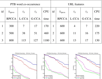
3.5
Experiments
In this section we compare several fast algorithms for computing CCA on large datasets.
• RPCCA : Instead of running CCA directly on the high dimensionalX Y, RPCCA
computes CCA only between the topkrpccaprinciple components (left singular
vec-tor) ofXandYwherekrpcca p1, p2. For largen, p1, p2, we use randomized
algo-rithm introduced in [28] for computing the top principle components ofX andY
(see appendix for details). The tuning parameter that controls the tradeoff between
computational cost and accuracy iskrpcca. Whenkrpcca is small RPCCA is fast but
fails to capture the correlation structure on the bottom principle components ofX
andY. Whenkrpccagrows larger the principle components captures more structure
inX Yspace but it takes longer to compute the top principle components. In the
experiments we varykrpcca.
• D-CCA : See section 3.3.1 for detailed descriptions. The advantage of D-CCA is
it’s extremely fast. In the experiments we iterate 30 times (t1 = 30) to make sure
D-CCA achieves convergence. As mentioned earlier, when Cxx and Cyy are far
from diagonal D-CCA becomes inaccurate.
• L-CCA : See Algorithm 6 for detailed description. We find that the accuracy of
LING in every orthogonal iteration is crucial to finding directions with large
cor-relation while a smallt1 suffices. So in the experiments we fixt1 = 5and varyt2.
In both experiments we fixkpc = 100 so the topkpc singular vectors of X,Yand
every LING iteration can be computed relatively fast.
in every iteration is computed directly by GD. G-CCA does not need to compute
top singular vectors ofXandYas L-CCA . But by equation 3.4.1 and remark 3.4.3
GD takes more iterations to converge compared with LING . Comparing G-CCA
and L-CCA in the experiments illustrates the benefit of removing the top singular
vectors in LING and how this can affect the performance of the CCA algorithm.
Same as L-CCA we fix the number of orthogonal iterationst1 to be 5 and varyt2,
the number of gradient iterations for solving LS.
RPCCA , L-CCA , G-CCA are all ”asymptotically correct” algorithms in the sense
that if we spend infinite CPU time all three algorithms will provide the exact CCA
so-lution while D-CCA is extremely fast but relies on the assumption thatX Yboth have
orthogonal columns. Intuitively, given a fixed CPU time, RPCCA dose an exact search
on krpcca top principle components of X and Y. L-CCA does an exact search on the
topkpcprinciple components (kpc < krpcca) and an crude search over the other directions.
G-CCA dose a crude search over all the directions. The comparison is in fact testing
which strategy is the most effective in finding large correlations over huge datasets.
Remark 3.5.1. Both RPCCA and G-CCA can be regarded as special cases of L-CCA
. When t1 is large and t2 is 0, L-CCA becomes RPCCA and when kpc is 0 L-CCA
becomes G-CCA .
In the following experiments we aims at extracting 20 most correlated directions from
huge data matrices X andY. The output of the above four algorithms are two n×20
Then a CCA is performed between Xkcca and Ykcca with matlab built-in CCA function.
The canonical correlations betweenXkcca andYkcca indicates the amount of correlations
captured from the the hugeX Yspaces by above four algorithms. In all the experiments,
we vary krpcca for RPCCA and t2 for L-CCA and G-CCA to make sure these three
algorithms spends almost the same CPU time ( D-CCA is alway fastest). The 20
canoni-cal correlations between the subspaces returned by the four algorithms are plotted (larger
means better).
We want to make to additional comments here based on the reviewer’s feedback.
First, for the two datasets considered in the experiments, classical CCA algorithms like
the matlab built in function takes more than an hour while our algorithm is able to get
an approximate answer in less than 10 minutes. Second, in the experiments we’ve been
focusing on getting a good fit on the training datasets and the performance is evaluated
by the magnitude of correlation captured in sample. To achieve better generalization
performance a common trick is to perform regularized CCA [31] which easily fits into
our frame work since it’s equivalent to running iterative ridge regression instead of OLS
in Algorithm 4. Since our goal is to compute a fast and accurate fit, we don’t pursue the